DOI:10.32604/cmc.2021.018040
| Computers, Materials & Continua DOI:10.32604/cmc.2021.018040 | |
| Article |
Pseudo Zernike Moment and Deep Stacked Sparse Autoencoder for COVID-19 Diagnosis
1School of Informatics, University of Leicester, Leicester, LE1 7RH, UK
2Department of Computer Science, HITEC University Taxila, Taxila, Pakistan
3Science in Civil Engineering, University of Florida, Gainesville, Florida, FL 32608, Gainesville, USA
4School of Mathematics and Actuarial Science, University of Leicester, LE1 7RH, UK
*Corresponding Author: Shui-Hua Wang. Email: shuihuawang@ieee.org
Received: 22 February 2021; Accepted: 07 April 2021
Abstract: (Aim) COVID-19 is an ongoing infectious disease. It has caused more than 107.45 m confirmed cases and 2.35 m deaths till 11/Feb/2021. Traditional computer vision methods have achieved promising results on the automatic smart diagnosis. (Method) This study aims to propose a novel deep learning method that can obtain better performance. We use the pseudo-Zernike moment (PZM), derived from Zernike moment, as the extracted features. Two settings are introducing: (i) image plane over unit circle; and (ii) image plane inside the unit circle. Afterward, we use a deep-stacked sparse autoencoder (DSSAE) as the classifier. Besides, multiple-way data augmentation is chosen to overcome overfitting. The multiple-way data augmentation is based on Gaussian noise, salt-and-pepper noise, speckle noise, horizontal and vertical shear, rotation, Gamma correction, random translation and scaling. (Results) 10 runs of 10-fold cross validation shows that our PZM-DSSAE method achieves a sensitivity of 92.06% ± 1.54%, a specificity of 92.56% ± 1.06%, a precision of 92.53% ± 1.03%, and an accuracy of 92.31% ± 1.08%. Its F1 score, MCC, and FMI arrive at 92.29% ±1.10%, 84.64% ± 2.15%, and 92.29% ± 1.10%, respectively. The AUC of our model is 0.9576. (Conclusion) We demonstrate “image plane over unit circle” can get better results than “image plane inside a unit circle.” Besides, this proposed PZM-DSSAE model is better than eight state-of-the-art approaches.
Keywords: Pseudo Zernike moment; stacked sparse autoencoder; deep learning; COVID-19; multiple-way data augmentation; medical image analysis
COVID-19 has caused more than 107.45 m confirmed cases and 2.35 m deaths till 11/Feb/2021 in about 192 countries/regions and 26 cruise/naval ships [1]. Fig. 1 shows the top 10 countries of cumulative confirmed cases and deaths, respectively. The main symptoms of COVID-19 are low fever, a new and ongoing cough, a loss or change to taste and smell [2]. In the UK, three vaccines are formally approved as Pfizer/BioNTech, Oxford/AstraZeneca, and Moderna. Two COVID-19 diagnosis methods are available. The former is viral testing to test the existence of viral RNA fragments [3]. The swab test shortcomings are two folds: (i) the swab samples may be contaminated, and (ii) it needs to wait from several hours to several days to get the test results. The latter is chest imaging. There are two main chest imaging available: chest computed tomography (CCT) [4] and chest X-ray (CXR) [5].
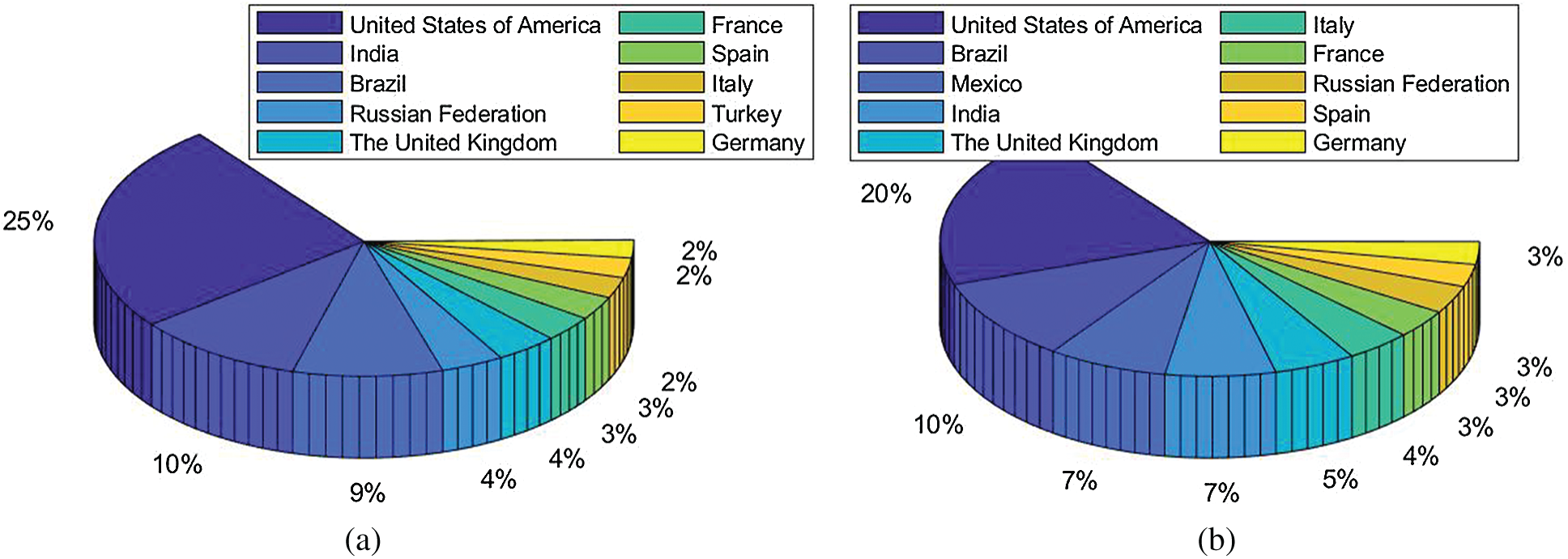
Figure 1: Data till 11/Feb/2021 (a) Cumulative confirmed cases (b) Cumulative deaths
CCT is one of the best chest imaging [6] techniques since it provides the finest resolution and can recognize extremely small nodules in the chest region. CCT employs computer-processed combinations of multiple X-ray observations taken from different angles [7] to produce high-quality 3D tomographic images (virtual slices). In contrast, CXR only provides one 2D image, which performs poorly on soft tissue contrast. This study focuses on the CCT images [8].
Currently, numerous studies are working on using machine learning (ML) and deep learning (DL) technologies [9,10]. For example, Guo et al. [11] employed ResNet-18 for classifying thyroid images. Lu [12] utilized an extreme learning machine (ELM) trained by bat algorithm (BA). Those two approaches were not developing for COVID-19, but they can be transferred to the COVID-19 dataset easily and used as comparison basis approaches in our experiments. For COVID-19 researches, Yao [13] proposed a wavelet entropy biogeography-based optimization (WEBBO) method for COVID-19 diagnosis. Wu [14] presented three-segment biogeography-based optimization (3SBBO) for recognizing COVID-19 patients. Wang et al. [15] presented a DeCovNet. Their accuracy achieved 90.1%. El-kenawy et al. [16] presented a novel feature selection voting classifier (FSVC) method for COVID-19 classification. Yu et al. [17] presented a GoogleNet-COD method to detect COVID-19. Chen [18] designed a gray-level co-occurrence matrix and support vector machine (GLCMSVM) method to classify COVID-19 images [19].
To further improve the performance of automatic COVID-19 diagnosis, this paper proposes a novel method that combines the traditional ML approach with the recent DL approach. We use the pseudo-Zernike moment (PZM) as the extracted features, and we use a deep-stacked sparse autoencoder (i.e., one of the deep neural networks) as the classifier. The combination achieves excellent results that overperform eight state-of-the-art approaches. The novelties of our paper lie in the following aspects
• We are the first to apply a pseudo-Zernike moment to COVID-19 image analysis.
• Deep stacked sparse autoencoder (DSSAE) works better than traditional classifiers.
• Our proposed “PZM-DSSAE” model is better than eight state-of-the-art approaches.
We use the dataset in reference [20], which contains 148 COVID-19 patients and 148 healthy control (HC) subjects. Slice level selection [20] was employed to generate
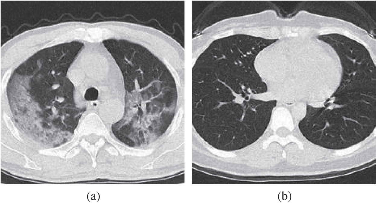
Figure 2: Example of preprocessed images (a) COVID-19 (b) HC
Tab. 1 displays the abbreviation list Image moment was firstly introduced by Hu [21], who used geometric moments to generate a set of invariants. Hu’s moments have been widely used in knee osteoarthritis classification [22], brain tumor classification [23], etc. However, geometric moments are sensitive to noise. Thus, Teague [24] introduced Zernike moments (ZMs) based on orthogonal Zernike polynomials. The orthogonal moments have been proven to be more robust in noisy conditions, and they can achieve a near-zero value of redundancy measure [25].

Later, pseudo Zernike moment (PZM) is derived from Zernike moment. PZMs have been proven to give better performances than other moment functions such as Hu moments, Zernike moments, etc. For example, for an order
The kernel of PZMs is a set of orthogonal pseudo-Zernike polynomials defined over the polar coordinate inside a unit circle (UC). The 2D PZM of order
where the pseudo-Zernike polynomials
where
Note that PZM are defined in terms of polar coordinates
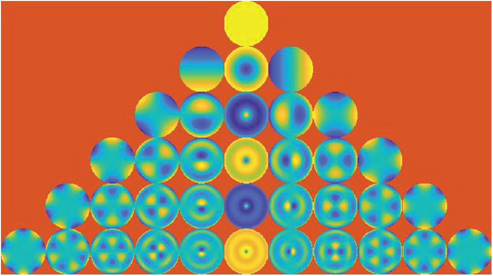
Figure 3: Pseudo Zernike functions of orders
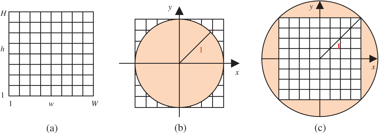
Figure 4: Two transformation (IP: image plane; UC: unit circle) (a) Raw image plane
Traditionally,
The fundamental element of DSSAE in the autoencoder (AE), which is a typical shallow neural network that learns to map its input
The structure of AE is displayed in Fig. 5, where the encoder part is with weight
where the output
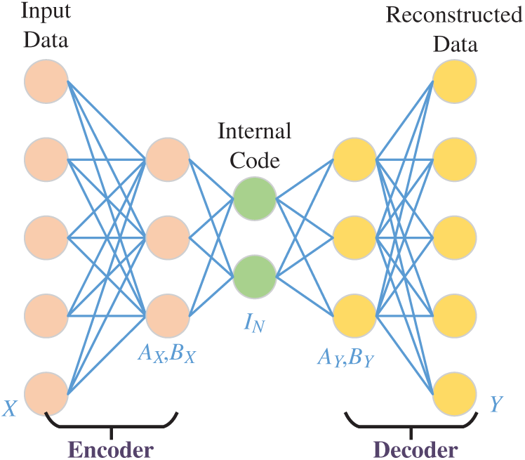
Figure 5: Structure of an AE
The sparse autoencoder (SAE) is a variant of AE. SAE encourages sparsity into AE. SAE only allows a small fraction of the hidden neurons to be active at the same time. To minimize the error between the input vector
where
where
To avoid over-complete mapping or learn a trivial mapping, we define one
where
where
The training procedure is set to scaled conjugate gradient descent (SCGD) method.
3.4 Deep Stacked Sparse Autoencoder
We use SAE as the building block and establish the final deep-stacked sparse autoencoder (DSSAE) classifier by following three operations: (i) We include input layer, preprocessing layer, PZM layer; (ii) We stack four SAEs; (iii) We append softmax layer at the bottom of our AI model. The details of this proposed PZM-DSSAE model are listed in Tab. 2 and illustrated in Fig. 6. After processing, all the CCT images are normalized to fixed grayscaled images with the size of

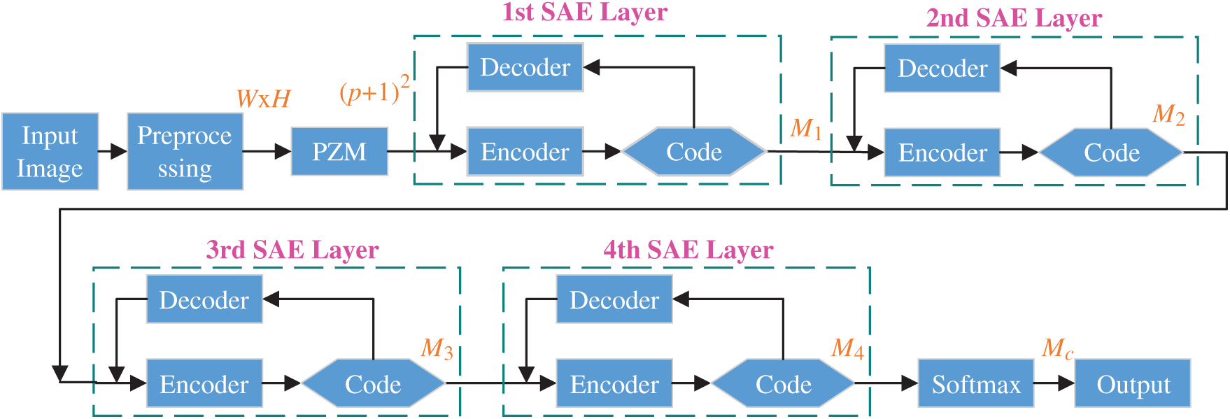
Figure 6: Structure of proposed PZM-DSSAE model
The small size of training images causes overfitting, one solution to data augmentation (DA) that creates fake training images. Multiple-way DA (MDA) is an enhanced method of DA. Wang [33] proposed a 14-way data augmentation, in which they employed seven different DA techniques on
In this study, we add two new DA techniques, speckle noise (SN) [34] and salt-and-pepper noise (SAPN). SN altered image is defined as
where
For the
where
First,
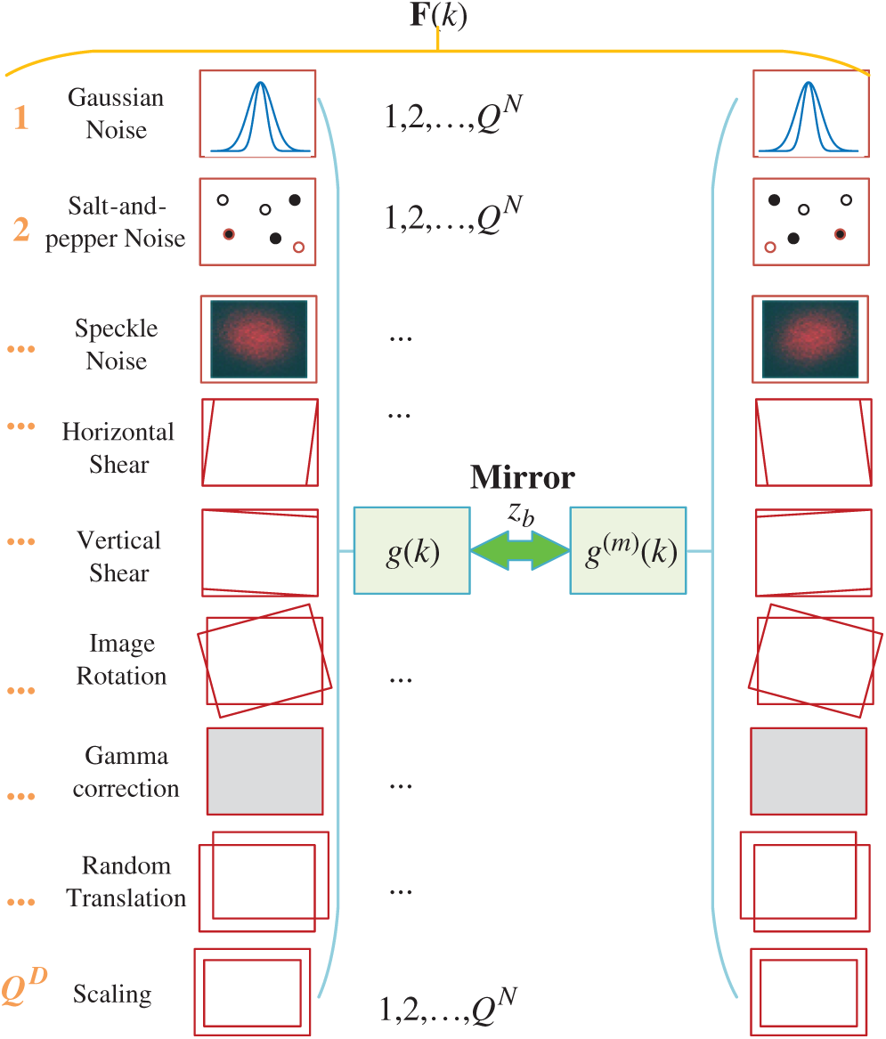
Figure 7: Diagram of proposed 16-way DA
Suppose
Second, horizontal mirrored image is generated as:
where
Third, all the
Fourth, the raw image
where
Algorithm 2 summarizes the pseudocode of proposed 18-way DA method.


Figure 8: F-fold cross validation
To avoid randomness, we run the whole above procedure
Note here the off-diagonal entries of
The first four measures are sensitivity, specificity, precision and accuracy, common in most pattern recognition papers. The last three measures are F1 score, Matthews correlation coefficient (MCC) [38], and Fowlkes–Mallows index (FMI) [39]. They are defined as:
Besides, the receiver operating characteristic (ROC) curve [40] is used to provide a graphical plot of our model. ROC curve is created by plotting the true positive rate against the false-positive rate at various threshold settings. The area under the curve (AUC) is also calculated.
Tab. 3 displays the parameter setting of this study. The number of samples of each class is 320. The minimum and maximum grayscale values are set to

4.2 Illustration of 18-Way Data Augmentation
Fig. 9 shows the
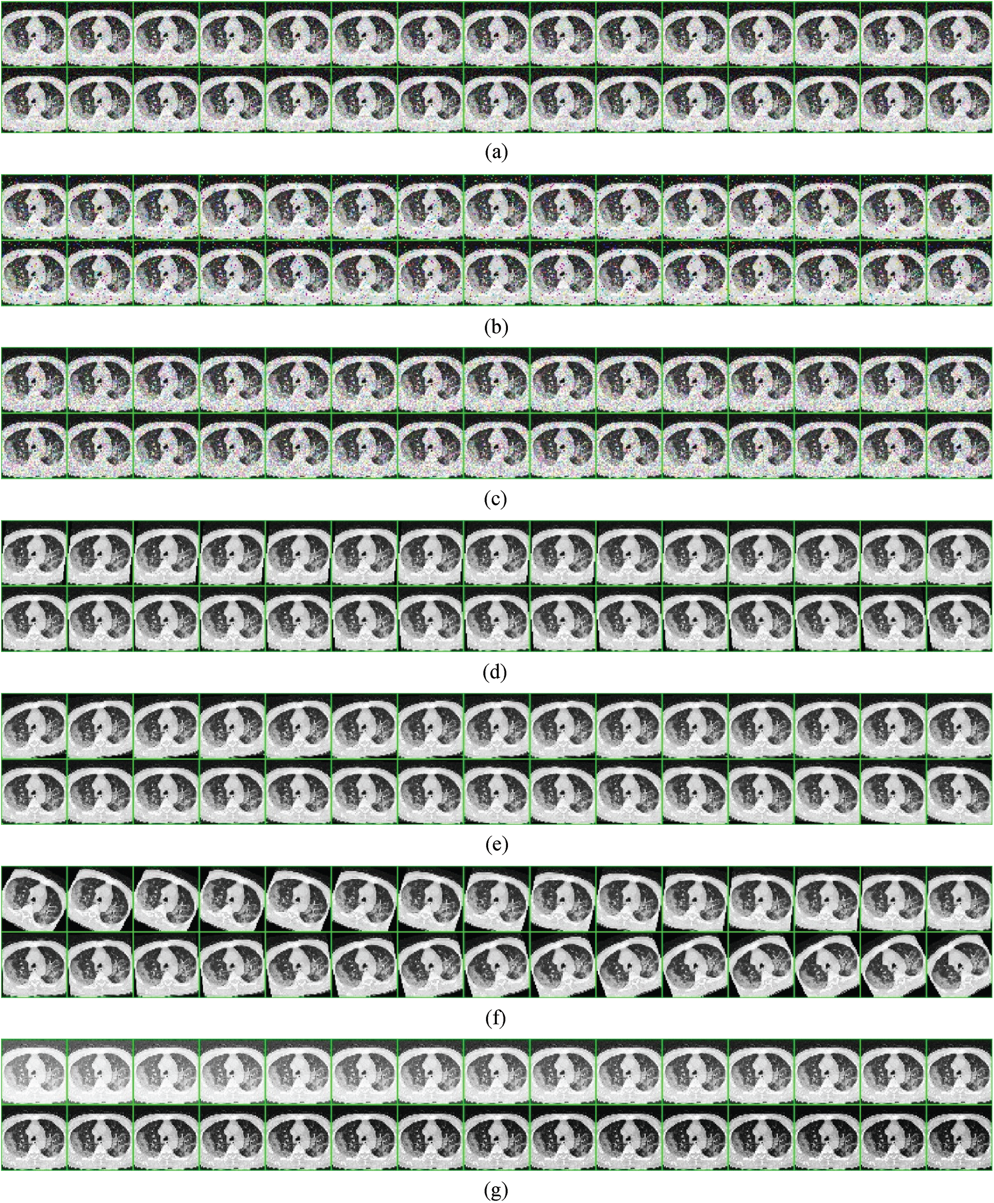
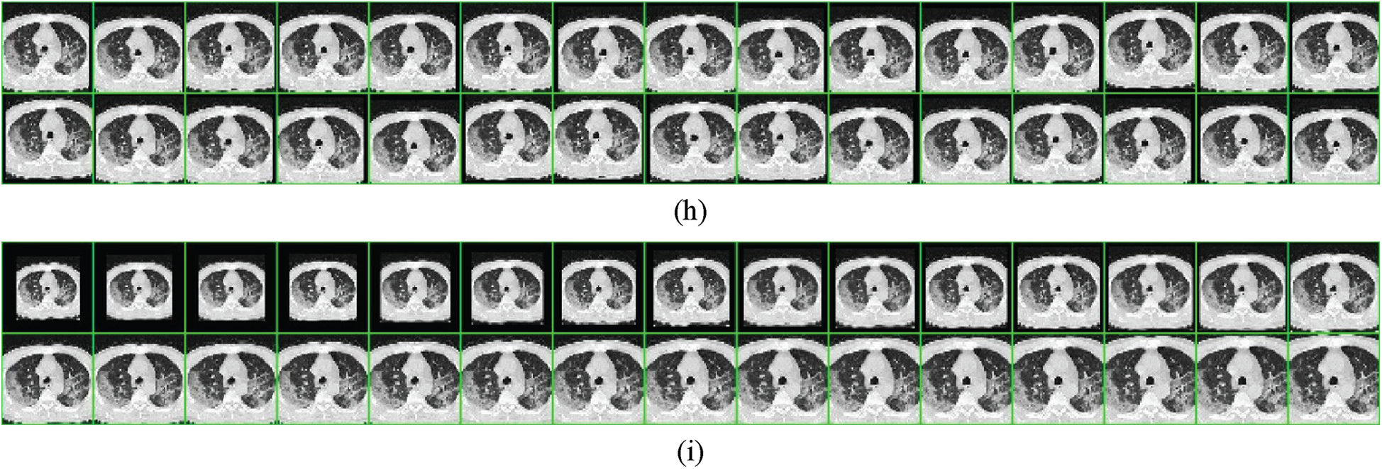
Figure 9:
4.3 Statistical Analysis and Transformation Comparison
Tab. 4 gives the 10 runs of 10-fold cross-validation, where we can see our method achieves a sensitivity of 92.06% ± 1.54%, a specificity of 92.56% ± 1.06%, a precision of 92.53% ± 1.03%, and an accuracy of 92.31% ± 1.08%. Its F1 score, MCC, and FMI arrive at 92.29% ± 1.10%, 84.64% ± 2.15%, and 92.29% ± 1.10%, respectively. The AUC is 0.9576.
In addition, we compared the two transformation settings: IP over UC against IP inside UC (See Fig. 4). The IP inside the UC setting achieves a sensitivity of 91.84% ± 2.18%, a specificity of 92.44% ± 1.31%, and an accuracy of 92.14% ± 1.12%, which are worse than IP over UC setting. This comparison result demonstrates the reason why we choose IP over UC in this study. Particularly, the receiver operating characteristics (ROC) curves of both settings are displayed in Fig. 10.

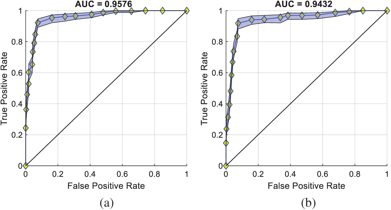
Figure 10: ROC curves of two settings (a) IP over UC (b) IP inside UC
4.4 Comparison to State-of-the-Art Methods
This proposed PZM-DSSAE method is compared with 8 state-of-the-art methods. The comparison results are carried out on the same dataset via 10 runs of 10-fold cross-validation, and the results are displayed in Tab. 5. Fig. 11 displays the error bar of the proposed method against 8 state-of-the-art methods. We can see that the proposed PZM-DSSAE gives the best performance among all the methods. The reason is three folds: (i) We try to use PZM as the feature descriptors, (ii) DSSAE is used as the classifier, (iii) 18-way DA is employed to solve the overfitting problem.

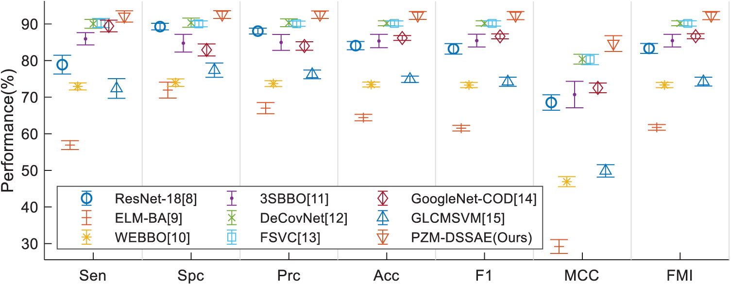
Figure 11: Error bar plot of method comparison
This study proposed a novel PZM-DSSAE system for COVID-19 diagnosis. As far as the authors’ best known, we are the first to apply PZM to COVID-19 image analysis. Also, two other improvements are carried out: (i) DSSAE is used as the classifier, and (ii) multiple-way data augmentation is employed to generalize the classifier. Our model yields a sensitivity of 92.06% ± 1.54%, a specificity of 92.56% ± 1.06%, an accuracy of 92.31% ± 1.08%, and an AUC of 0.9576.
In the future, we shall collect more COVID-19 images from more patients and multiple modalities. Also, other advanced AI models will be tested, such as graph neural networks and attention networks.
Funding Statement: This study was supported by Royal Society International Exchanges Cost Share Award, UK (RP202G0230); Medical Research Council Confidence in Concept Award, UK (MC_PC_17171); Hope Foundation for Cancer Research, UK (RM60G0680); Global Challenges Research Fund (GCRF), UK (P202PF11)
Conflicts of Interest: The authors declare that they have no conflicts of interest to report regarding the present study.
1. B. Zemrani, M. Gehri, E. Masserey, C. Knob and R. Pellaton, “A hidden side of the COVID-19 pandemic in children: The double burden of undernutrition and overnutrition,” International Journal for Equity in Health, vol. 20, no. 1, pp. 4, 2021. [Google Scholar]
2. M. Bassi, L. Negri, A. Delle Fave and R. Accardi, “The relationship between post-traumatic stress and positive mental health symptoms among health workers during COVID-19 pandemic in Lombardy,” Italy Journal of Affective Disorders, vol. 280, pp. 1–6, 2021. [Google Scholar]
3. D. Simiies, A. R. Stengaard, L. Combs, D. Raben and T. C. I. A. Euro, “Impact of the COVID-19 pandemic on testing services for HIV, viral hepatitis and sexually transmitted infections in the WHO European Region, march to august 2020,” Eurosurveillance, vol. 25, pp. 7, 2020. [Google Scholar]
4. F. Salahshour, M.-M. Mehrabinejad, M. N. Toosi, M. Gity, H. Ghanaati et al., “Clinical and chest CT features as a predictive tool for COVID-19 clinical progress: Introducing a novel semi-quantitative scoring system,” European Radiology, vol. 11, pp. 1–11, 2021. [Google Scholar]
5. A. M. Ismael and A. Sengur, “The investigation of multiresolution approaches for chest X-ray image based COVID-19 detection,” Health Information Science and Systems, vol. 8, no. 1, pp. 1–13, 2020. [Google Scholar]
6. A. Hata, M. Yanagawa, Y. Yoshida, T. Miyata, N. Kikuchi et al., “The image quality of deep-learning image reconstruction of chest CT images on a mediastinal window setting,” Clinical Radiology, vol. 76, no. 2, pp. 9, 2021. [Google Scholar]
7. Y. Satoh, U. Motosugi, M. Imai, Y. Omiya and H. Onishi, “Evaluation of image quality at the detector’s edge of dedicated breast positron emission tomography,” Ejnmmi Physics, vol. 8, no. 1, pp. 14, 2021. [Google Scholar]
8. M. A. Khan, S. Kadry, Y.-D. Zhang, T. Akram, M. Sharif et al., “Prediction of COVID-19-pneumonia based on selected deep features and one class kernel extreme learning machine,” Computers & Electrical Engineering, vol. 90, pp. 106960, 2021. [Google Scholar]
9. T. Akram, M. Attique, S. Gul, A. Shahzad, M. Altaf et al., “A novel framework for rapid diagnosis of COVID-19 on computed tomography scans,” Pattern Analysis and Applications, pp. 1–14, 2021. https://doi.org/10.1007/s10044-020-00950-0. [Google Scholar]
10. H. T. Rauf, M. I. U. Lali, M. A. Khan, S. Kadry, H. Alolaiyan et al., “Time series forecasting of COVID-19 transmission in Asia Pacific countries using deep neural networks,” Personal and Ubiquitous Computing, vol. 8, pp. 1–18, 2021. [Google Scholar]
11. M. H. Guo and Y. Z. Du, “Classification of thyroid ultrasound standard plane images using ResNet-18 networks,” in IEEE 13th Int. Conf. on Anti-Counterfeiting, Security, and Identification, Xiamen, China, pp. 324–328, 2019. [Google Scholar]
12. S. Lu, “A pathological brain detection system based on extreme learning machine optimized by Bat algorithm,” CNS & Neurological Disorders-Drug Targets, vol. 16, no. 1, pp. 23–29, 2017. [Google Scholar]
13. X. Yao, “COVID-19 detection via wavelet entropy and biogeography-based optimization,” in {COVID-19}: Prediction, Decision-Making, and Its Impacts, K. C. Santosh, A. Joshi (Eds.Cham: Springer, pp. 69–76, 2020. [Google Scholar]
14. X. Wu, “Diagnosis of COVID-19 by wavelet renyi entropy and three-segment biogeography-based optimization,” International Journal of Computational Intelligence Systems, vol. 13, no. 1, pp. 1332–1344, 2020. [Google Scholar]
15. X. G. Wang, X. B. Deng, Q. Fu, Q. Zhou, J. P. Feng et al., “A weakly-supervised framework for COVID-19 classification and lesion localization from chest CT,” IEEE Transactions on Medical Imaging, vol. 39, no. 8, pp. 2615–2625, 2020. [Google Scholar]
16. E. S. M. El-kenawy, A. Ibrahim, S. Mirjalili, M. M. Eid and S. E. Hussein, “Novel feature selection and voting classifier algorithms for COVID-19 classification in CT images,” IEEE Access, vol. 8, pp. 179317–179335, 2020. [Google Scholar]
17. X. Yu, S.-H. Wang, X. Zhang and Y.-D. Zhang, “Detection of COVID-19 by GoogLeNet-COD,” in Int. Conf. on Intelligent Computing, Bari, Italy, pp. 499–509, 2020. [Google Scholar]
18. Y. Chen, “Covid-19 classification based on gray-level co-occurrence matrix and support vector machine,” in COVID-19: Prediction, Decision-Making, and Its Impacts, K. C. Santosh, A. Joshi (Eds.Singapore: Springer, Cham, pp. 47–55, 2020. [Google Scholar]
19. M. A. Khan, N. Hussain, A. Majid, M. Alhaisoni, S. A. C. Bukhari et al., “Classification of positive COVID-19 CT scans using deep learning,” Computers, Materials and Continua, vol. 66, no. 2, pp. 1–15, 2021. [Google Scholar]
20. Y. D. Zhang, “A seven-layer convolutional neural network for chest CT based COVID-19 diagnosis using stochastic pooling,” IEEE Sensors Journal, vol. 1, pp. 1, 2021. [Google Scholar]
21. M.-K. Hu, “Visual pattern recognition by moment invariants,” IRE Transactions on Information Theory, vol. 8, pp. 179–187, 1962. [Google Scholar]
22. S. S. Gornale, P. U. Patravali and P. S. Hiremath, “Automatic detection and classification of knee osteoarthritis using Hu’s invariant moments,” Frontiers in Robotics and AI, vol. 7, pp. 8, 2020. [Google Scholar]
23. S. Ouchtati, A. Chergui, S. Mavromatis, B. Aissa and J. Sequeira, “Novel method for brain tumor classification based on use of image entropy and seven Hu’s invariant moments,” Traitement Du Signal, vol. 36, no. 6, pp. 483–491, 2019. [Google Scholar]
24. M. R. Teague, “Image analysis via the general theory of moments,” Journal Optical Soceity America, vol. 70, no. 8, pp. 920–930, 1980. [Google Scholar]
25. A. Grosso and T. Scharf, “Scalar analytical expressions for the field dependence of Zernike polynomials in asymmetric optical systems with circular symmetric surfaces,” OSA Continuum, vol. 3, no. 10, pp. 2749–2765, 2020. [Google Scholar]
26. C. W. Chong, P. Raveendran and R. Mukundan, “The scale invariants of pseudo-Zernike moments,” Pattern Analysis and Applications, vol. 6, no. 3, pp. 176–184, 2003. [Google Scholar]
27. N. Borzue, K. Faez and IEEE, “Object contour detecting using pseudo zernike moment and multi-layer perceptron,” in 22nd Iranian Conf. on Biomedical Engineering, Tehran, Iran, pp. 304–308, 2015. [Google Scholar]
28. S. P. Singh and S. Urooj, “An improved CAD system for breast cancer diagnosis based on generalized pseudo zernike moment and Ada-DEWNN classifier,” Journal of Medical Systems, vol. 40, no. 4, pp. 1–23, 2016. [Google Scholar]
29. S. Du, “Alzheimer’s disease detection by pseudo zernike moment and linear regression classification,” CNS & Neurological Disorders-Drug Targets, vol. 16, no. 1, pp. 11–15, 2017. [Google Scholar]
30. Y. Jiang, “Exploring a smart pathological brain detection method on pseudo Zernike moment,” Multimedia Tools and Applications, vol. 77, no. 17, pp. 22589–22604, 2018. [Google Scholar]
31. D. K. Mohanty, A. K. Parida and S. Suman, “Financial market prediction under deep learning framework using auto encoder and kernel extreme learning machine,” Applied Soft Computing, vol. 99, no. 3, pp. 14, 2021. [Google Scholar]
32. J. Lequesne and P. Regnault, “vsgoftest: An R package for goodness-of-fit testing based on Kullback–Leibler divergence,” Journal of Statistical Software, vol. 96, no. Code Snippet 1, pp. 26, 2020. [Google Scholar]
33. S.-H. Wang, “Covid-19 classification by FGCNet with deep feature fusion from graph convolutional network and convolutional neural network,” Information Fusion, vol. 67, pp. 208–229, 2021. [Google Scholar]
34. C. Buitrago-Duque, R. Castaneda and J. Garcia-Sucerquia, “Pointwise phasor tuning for single-shot speckle noise reduction in phase wave fields,” Optics and Lasers in Engineering, vol. 137, pp. 5, 2021. [Google Scholar]
35. K. Vasanth and R. Varatharajan, “An adaptive content based closer proximity pixel replacement algorithm for high density salt and pepper noise removal in images,” Journal of Ambient Intelligence and Humanized Computing, vol. 3, pp. 1–15, 2020. [Google Scholar]
36. D. Muller and F. Kramer, “MIScnn: A framework for medical image segmentation with convolutional neural networks and deep learning,” BMC Medical Imaging, vol. 21, pp. 11, 2021. [Google Scholar]
37. J. Radoux and P. Bogaert, “About the pitfall of erroneous validation data in the estimation of confusion matrices,” Remote Sensing, vol. 12, pp. 23, 2020. [Google Scholar]
38. D. Dreizin, F. Goldmann, C. LeBedis, A. Boscak, M. Dattwyler et al., “An automated deep learning method for tile AO/OTA pelvic fracture severity grading from trauma whole-body CT,” Journal of Digital Imaging, vol. 21, pp. 1–13, 2021. [Google Scholar]
39. R. Jena, B. Pradhan and A. M. Alamri, “Susceptibility to seismic amplification and earthquake probability estimation using recurrent neural network model in Odisha,” India Applied Sciences-Basel, vol. 10, pp. 18, 2020. [Google Scholar]
40. A. T. Young, K. Fernandez, J. Pfau, R. Reddy, N. A. Cao et al., “Stress testing reveals gaps in clinic readiness of image-based diagnostic artificial intelligence models,” NPJ Digital Medicine, vol. 4, pp. 8, 2021. [Google Scholar]
 | This work is licensed under a Creative Commons Attribution 4.0 International License, which permits unrestricted use, distribution, and reproduction in any medium, provided the original work is properly cited. |