DOI:10.32604/cmc.2021.018230
| Computers, Materials & Continua DOI:10.32604/cmc.2021.018230 | |
| Article |
Denoising Medical Images Using Deep Learning in IoT Environment
1School of Computer Science and Engineering, Lovely Professional University, Jalandhar, India
2Software Department, Sejong University, Seoul, Korea
3College of Computer Engineering and Sciences, Prince Sattam bin Abdulaziz University, Al-Kharj, 11942, Saudi Arabia
4Department of Information Technology, Faculty of Computing and Information Technology in Rabigh, King Abdulaziz University, Jeddah, 21911, Saudi Arabia
*Corresponding Author: Oh-Young Song. Email: oysong@sejong.edu
Received: 01 March 2021; Accepted: 02 April 2021
Abstract: Medical Resonance Imaging (MRI) is a noninvasive, nonradioactive, and meticulous diagnostic modality capability in the field of medical imaging. However, the efficiency of MR image reconstruction is affected by its bulky image sets and slow process implementation. Therefore, to obtain a high-quality reconstructed image we presented a sparse aware noise removal technique that uses convolution neural network (SANR_CNN) for eliminating noise and improving the MR image reconstruction quality. The proposed noise removal or denoising technique adopts a fast CNN architecture that aids in training larger datasets with improved quality, and SARN algorithm is used for building a dictionary learning technique for denoising large image datasets. The proposed SANR_CNN model also preserves the details and edges in the image during reconstruction. An experiment was conducted to analyze the performance of SANR_CNN in a few existing models in regard with peak signal-to-noise ratio (PSNR), structural similarity index (SSIM), and mean squared error (MSE). The proposed SANR_CNN model achieved higher PSNR, SSIM, and MSE efficiency than the other noise removal techniques. The proposed architecture also provides transmission of these denoised medical images through secured IoT architecture.
Keywords: Medical resonance imaging; convolutional neural network; denoising; contrast enhancement; internet of things; rheumatoid arthritis
In recent years, the global death rate has drastically increased due to medical conditions such as cardiovascular diseases, sinusitis (sinus infection), rheumatoid arthritis (RA) [1], and hematoma, etc. Identifying these diseases in the early stages aids in clinical diagnosis and reduction of the mortality rate to a great extent. In the last few years, the detection of cardiovascular disease [2], RA, and sinusitis has increased due to advances in imaging techniques such as magnetic resonance imaging (MRI). MRI has become popular because of its nonradioactive and noninvasive nature, precise high-resolution quality, and ability to diagnosis versatile diseases. MRI can be widely utilized in cardiac diagnosis due to its precise deformation detection in the myocardium and its surrounding tissues [3]. Furthermore, it can be widely used in many applications such as the detection of local myocardial strain and motion; angiography, arterial spin labelling; diagnosis of heart attack; [4] and diagnosis of lung, breast, and colorectal cancer.
However, MRI is associated with several drawbacks that degrade its performance such as limited spatial resolution, large encoding, huge image set, large power requirement, and high temporal dimensions [5,6,7]. In the last decade, many researchers have attempted to limit these drawbacks through MRI-related techniques such as compression sensing (CS), dictionary learning with block matching, wavelet techniques. However, MR image recovery is not as efficient as required because of the low-resolution quality of the image and the long time taken by many existing techniques to eliminate noise and reconstruct MR image sets. The MRI speed is limited due to physiological nerve stimulation, amplitude, and slew constraints.
CS is widely adopted and appreciated by many researchers due to its capability to reduce data acquisition time during MRI [8,9,10,11], magnetic validation and sensitivity analysis using a diffusion-weighted approach for the diagnosis of MR images. Reference [12] used low-rank matrix approximation for processing dynamic MR images. A sequential dictionary learning algorithm was used for functional MR images from correlated data to obtain the correlation between spatial and temporal smoothness [13]. However, the aforementioned techniques have several issues such as high nuclear relaxation time, normalization and optimization problems, realistic electromagnetic issues, large power consumption during diagnosis [14], and most importantly, long processing time leading to performance degradation of the system.
The low visual quality of the MR images provides inaccurate information and diagnosis for the treatment. These images captured during the acquisition process are prone to electromagnetic signals, reminisce the reflexes, are of irregular brightness and induce some artifacts. The artifacts may be in-the form of noise, labels, and low contrast. In this article, we proposed a convolution neural network (CNN) framework combined with a dictionary algorithm for removing noise, maintaining the contrast, and preserving the details within an image.
To resolve the problems of contrast and noise in MR image, an efficient and speedy algorithm that can easily handle large medical image processing is required. In recent years, the CNN technique has emerged as the most promising technique for handling large image datasets due to its robust feed-forward methods and easy training. It can reduce the drawbacks of contrast and noise present in MR images and reconstruct the image. It can train large image datasets faster and more precisely as it can perform parallel graphics processing unit (GPU) computing using a compute unified device architecture (CUDA) programming framework. Therefore, these special properties make the CNN architecture considerably different from those of other modern techniques mentioned in the literature. The present study is aimed at solving speed and high-quality reconstruction issues relating to medical images to maintain high performance. Speed is important factor in medical imaging due to its bulky image sets and the need to transfer these image sets to other stations. There is a chance of misbehaving reconstruction efficiency with increasing processing speed. Therefore, high-quality reconstruction with high speed is a very essential process in medical resonance imaging (especially MRI).
Therefore, in this paper, we present a sparse aware noise removal (SARN) technique that uses CNN for reconstructing high-quality MR images. The SANR_CNN model reduces various noises such as additive white gaussian (AWG), Rician, and speckle noise in MR images. A dictionary learning algorithm, which is a subject-based patch extraction method, is integrated with sparse representation to denoise the MR images. It also increases accuracy (reduces error) and eliminates computational complexity. Our SARN model, which is based on the CNN architecture, eliminates sparse optimization and redundancy problems. It subdivides the input image into various patches and passes it to the CNN architecture. Their difference is then fed to the training phase to generate a dictionary and these generated dictionaries are used in the testing phase to generate a high-quality image. In this way, our model eliminates various noises and outperforms all.
In India, 73 per cent of the population stays in rural areas and 80 per cent of trained physicians stays in urban areas. Therefore, to bridge a gap between rural and urban areas, cloud-based remote magnetic resonance imaging technologies and computer-aided diagnostics (CADs) are served. This architecture provides access to physicians anywhere in the world to facilitate the patients with proper diagnosis and security to medical images. This paper is organized in the following sections which are as follows. In Section 2, we described our proposed methodology. In Section 3, experimental results and evaluation are demonstrated and Section 4 concludes our paper.
A few methods for contrast and noise estimation are available and studied thoroughly in the literature. The fuzzy model proposed by authors in [15] was the practical method among noise identifiers used in image processing. Linear and quadratic indices were used in this method for measuring noise variance. An improved fuzzy histogram with bi-level equalization was proposed by authors in [16] for estimating quantitative parameters on gray images for preserving the brightness and feature similarity index. A Gaussian mixture model proposed by authors in [15] provided image reconstruction with partial discreteness. The robust principal component analysis (RPCA) used for reconstructing MR images has many drawbacks. Thus, a nonconvex method that solved problem of optimization on dynamic cardiac magnetic resonance data was proposed by authors in [12].
Authors in [17] implemented the data acquisition process on MR images with a total variation model. In this model, the idea of computing sensing and an iterative algorithm were used for tackling the optimization problem. The sensing approach proposed by author in [18] was combined with a low-dimensional model for exploiting the similarity and redundancy of MRI. Authors in [19] measured the gradient difference between two similar images to restore a high-resolution image with edge preservation. The similarity patches were deployed to estimate the intensity values. A combination of backpropagation filters was used for increasing the reconstructed image quality. Authors in [20] proposed a CNN-based automatic window to reduce the spatial resolution of images; this window used a space depth inference process to increase the execution time. The feature engineering process and tensor flow module were automatically imposed practically with a series of CNN building blocks.
The feed-forward neural network for removal of Rician noise was implemented by author in [21]. This model was imposed on a single-level noise with subintervals for training and demonstrated mutual information. Sparse tensors with a reweighted factor and an improved Split Bregman scheme were an efficient implementation by author in [22]. However, this model lacks computational time compared with other models. In [23] author proposed a filter, Kolmogorov-Smirnov based distance, for finding similar patches or pixels within an image. The cumulative distribution function of different pixels was estimated and similarity was measured during the acquisition process. Authors in [24] proposed a few nonlocal means (NLM) techniques that provided higher efficiency and other denoising parameters. In this model, the three-dimensional (3D) NLM provided higher PSNR and SSIM values, but the adaptive multiresolution technique provided higher accuracy for the contrast factor. A model developed by authors in [13] by using partial separability and sparsity was utilized with highly under sampled space data. The image contrast enhancement was improved using an artificial bee colony method proposed by author in [25]. The transformation function combined with the method and extensive experiment were used for improving visual quality.
The neural network and optimal bilateral filter used by authors in [18] denoised the image. The obtained PSNR and RMSE values were considerably higher than some classifiers. The block matching 3D method proposed by Hanchate and Joshi gave improved contrast and removed the noise from PD and T1-weighted images in [26]. The block method which is based on a differential filter implemented by authors in [27] for noise removal, estimated the intensity of block difference of the images. Moreover, histograms were utilized for contrast improvement in the images. One of the methods proposed by authors in [28] used the average intensity of each image applied on fluid attenuation inversion recovery (FLAIR) images that were contaminated with white matter hyperintensities (WMH). The CNN model enabled the extraction of some high-level features from different images. This model proposed by author in [29] outperforms total variation (TV) and block matching three dimensional (BM3D) methods as determined through a statistical test conducted for assessment and calculation of the diffusion parameter.
The IoT based computing is used to solve or reduce the complexity of applications [30]. To compute low-resolution images, that involves multi-resolution processing compressed sensing reconstruction algorithm was proposed. The patients’ data is stored in cloud with cryptographic model and optimization approach [31]. The optimal key is chosen using hybrid swarm optimization compared with diverse algorithms. The deep neural network used in [32] to synthesize data that captures representations with multi-style data learning. This approach mitigates the cost and time into IoT.
We used a SARN technique with a CNN architecture to reconstruct high-quality MR images. Our model consists of the following phases: dictionary creation phase, combining sparse coding into the dictionary stage, and parametric reconstruction quality evaluation phase.
An input image is subdivided into various sparse layers in the dictionary creation stage. Every image is divided into several different patches, which are then fed into our SANR_CNN model. The output is used in the training stage to construct a dictionary. In the next stage, the sparse aware denoising and reconstruction technique is adopted with dictionary learning methods and the constructed dictionary is used in testing to eliminate noise. Thus, a high-quality medical MR image is generated. In the last stage, the quality of the reconstructed image is evaluated based on PSNR and SSIM. Our experimental results demonstrate the high resolution of the reconstructed image.
An abundant amount of huge MR images is available in real-time that need to transferred and reconstructed at other stations. However, modern techniques have certain limitations such as high temporal dimensions, large power absorption, huge image dataset, and high slew-rate, and low processing speed. Therefore, two techniques adopted in our model to evaluate high reconstruction quality, maintain high processing speed, and eliminate noise were the SARN_CNN and reconstruction technique in integration with dictionary learning method.
3.1 Secure Transmission Module
IoT-enabled magnetic resonance imaging system architecture is illustrated in Fig. 1. This provides medical facilities for rural people by transmitting MRI data to the cloud, which physicians can then access remotely for diagnostic purposes. Fig. 1a, shows the workflow of CAD module, after denoising the images can be stored and accessed by physicians provided with login credentials. The communication modules directly connect to cloud service provider to exchange the data with existing connection establishment like ethernet or Wi-Fi. The remote device or devices connect through gateway protocol acting as intermediate between devices and cloud services.
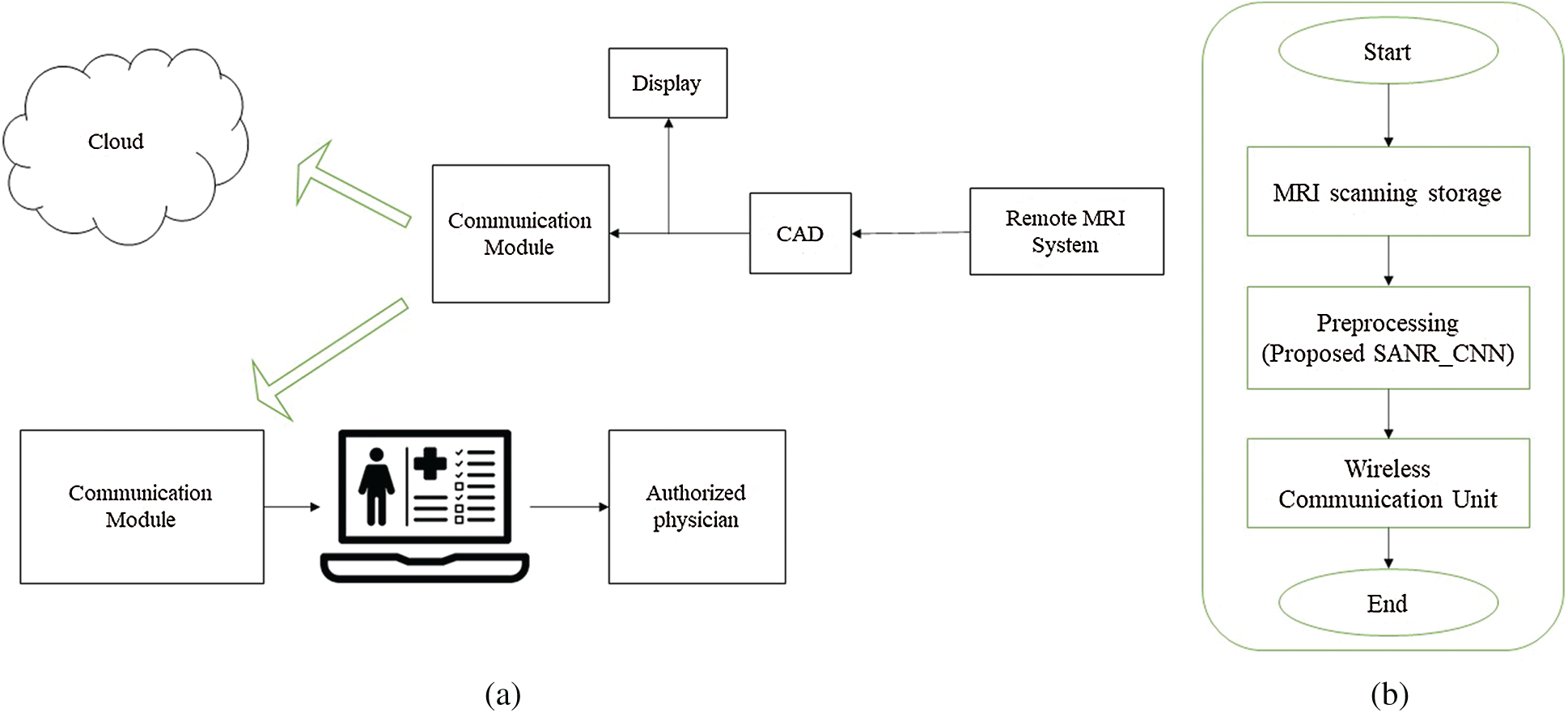
Figure 1: Proposed IoT architecture with pre-processing. (a) IoT communication module (b) workflow of proposed CAD system with pre-processing step
The end-to-end encryption and decryption are performed with attribute-based encryption (ABE). Attribute-based Encryption is an expanded Identity-based Encryption concept (IBE). ABE is grounded on the Attribute Knowledge Community and Access Tree for encryption. ABE is a cryptographic algorithm that only a user with sufficient attribute value for encrypted data can decrypt this data. The Access Tree may be used to choose whether or not to allow access to the data. In this paper cipher text-policy attribute-based encryption has four components such as setup, encryption, decryption and keygen.
Setup(1n) outputs Mk (master key) and Pk (pubic key). The setup algorithm selects bilinear group B0 and generator g. Then it randomly chooses two parameters α, β, where Pk = B0, and Mk = (β, gα).
Encrypt outputs the cipher text (CT) corresponding a message given with public key and access tree. The algorithm chooses each node of the tree with a polynomial qx, starting from root node following top-down approach. Then cipher text is computed with CT = (T,
Decrypt outputs the message M corresponding the cipher text CT. An attribute I = attrib (x), where the node x is a leaf node. DT = (CT, x) = e(g, g)rs.
Keygen outputs secret key (Sk) with input a set of attributes S and a random number r, are chosen for each attribute j Sk = (D= g(α+r)/β), where D = gr.
3.2 Noise Model and Distribution
The noise was represented and estimated using the intensity of each pixel by pixel. The noise was represented using a probability distribution function (PDF) with the pixel intensity given in Eq. (1).
where, A is the original pixel intensity and M is the present pixel intensity.
I0 = Bessel function of zeroth order.
Σ = Standard deviation of Gaussian noise.
In Eq. (2), the noise within the range of 1–3 is Rician noise, the noise above value is 3 leads to Gaussian noise and the noise below the lowest value 1 corresponds to Rayleigh noise. The Rician noise is usually represented by Eq. (3)
where, Ym and Yre are imaginary and actual values, respectively. The values are affected by ξ1 and ξ2, where ξ1 and ξ2 are Gaussian noise with mean 0 and standard deviation σ.
where I, is the initial image, and ϴ is the phase value. A noisy image is signified as a scale of the raw image, represented by Eq. (6). The square of the magnitude is Rician noise calculated in the image by Eq. (7).
3.3 Pre-Processing Using SANR_CNN
Neural Networks work on the learned image statistics. Many researchers have recently shown their interest in neural networks, especially the CNN due to its high-quality reconstruction and denoising capability. It can easily handle large processing and performs various tasks such as traffic sign recognition, artificial neural networks, and medical image diagnosis, with the help of its pure feed-forward methods and efficient training. The CNN mainly focuses on the analysis of image data. The CNN architecture has a hierarchical structure and various hidden layers are present, in, deep learning CNN techniques. A special CNN was adopted with sparse logistics to denoise and create high-quality MR images by using dictionary learning methods. The CNN architecture can denoise images based on prior knowledge and efficient training regardless of noise type.
A medical image noise removal and reconstruction architecture is presented using model the SANR_CNN model in Fig. 3. The input image was subdivided into various patches and then passed to the SANR_CNN architecture, and the result was used in the training stage to create a dictionary. This was further used in the testing stage to eliminate noise and added with the input image, and a denoised reconstructed image was constructed. It consisted of two stages: a training stage and a testing stage. The proposed model as shown in Fig. 2 has 17 hidden layers. It consists of three kinds of layers; Conv, ReLU, and dilated network. The first and sixteenth layers are Conv and ReLU. The second, fifth, ninth, and twelfth layers are dilated convolution. The final layer is Conv with convolutional kernel of size 128 × 1 × 40 × 40 for first and final layer and 128 × 64 × 40 × 40 for other layers.
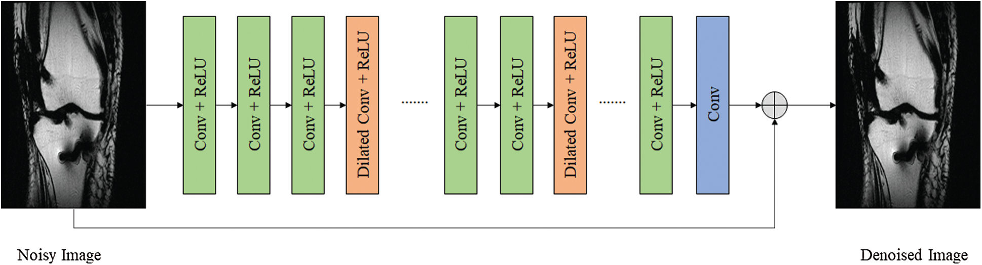
Figure 2: Proposed CNN model with dilated layers
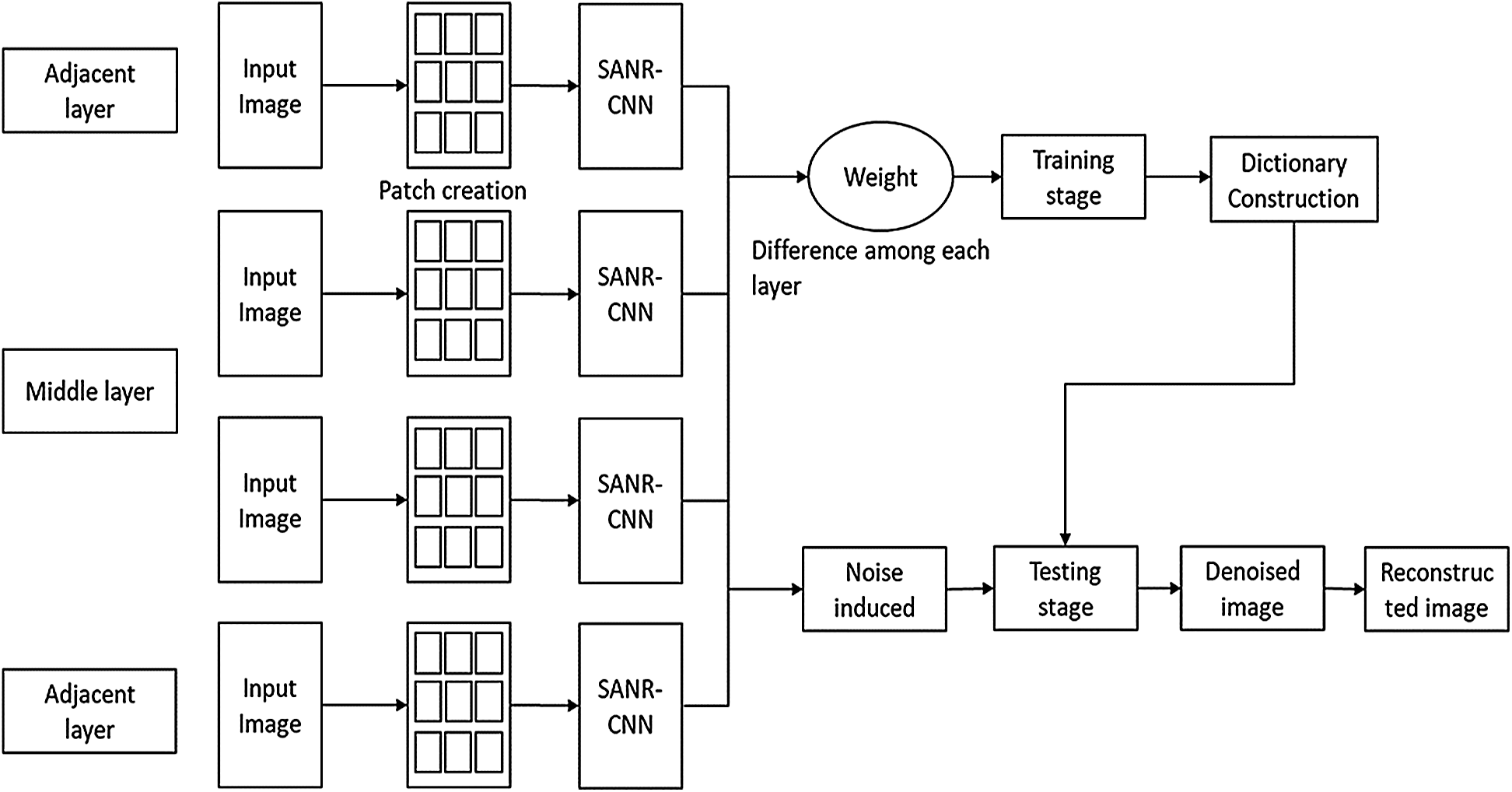
Figure 3: Noise removal and reconstruction architecture using SANR_CNN
Training is the most essential stage that dictates the control flow for image data analysis. Efficient training can always ensure high performance of any system. However, it is a large and complex process that takes a large amount of time to train image data. Therefore, an efficient technique is needed to train image data at an incredibly faster rate and very less processing time. In training, samples are repeatedly drawn and parameter selection is an arbitrary process. However, a better architecture is needed for effective performance. Hence, the study presented an efficient SARN and reconstruction technique based on the CNN architecture to obtain a denoised image.
In the study we used parallel GPU computing using the CUDA programming framework, to train large medical images at a considerably faster rate. The parameters were estimated on basis of the noise type and patches. More time was needed to train high-dimensional data. Regularization can be achieved using pretraining and small normalization vectors are easier to change. Our model was trained on greyscale medical images and can be trained on different noisy images to provide a high-quality denoised image. For training in the model SANR_CNN model, we used the difference between every layer to generate weights, and then, it is passed to the training phase. The dictionary is then created, which helps in achieving quality denoising for the input image with patches and reduces noise completely. In this way, we can compute effective training on large datasets and our experimental outcomes verify our training efficiency by outperforming all standard image denoising algorithms considering performance metrics such as PSNR, MSE, and SSIM. The model was trained with 1200 knee magnetic resonance images with the size of 512 × 512 pixels. Tab. 1 describes the dataset used for proposed model. 480 images of T1-weighted, 590 images of T2-weighted, and 130 FLAIR images.
The Dictionary learning technique is presented to give support to the denoising technique to obtain a denoised image. Let noise k be merged with the input image patch signal i in the Eq. (8),
Here, patch-wise denoising is computed. Size of each patch is taken as m*m, where k more often lies between 8 and 12. All the patches are individually denoised and a reconstructed image is then constructed by integrating altogether inside a frame. Overlapped patches are being optimized using the fusion process. Dictionary, D, whose size is considered as m2*n where, n > m2 on which our dictionary is based.
In a dictionary learning process, feature element sets are being provided as an initialization operation. A sparse linear reconstruction technique is used to denoise all noisy patches extracted from an image. In Eq. (9), the AWG noisy error can be reduced as,
where, a pre-defined factor is provided as
The dictionary learning scheme evaluates the high reconstruction quality image. Therefore, the probable possibilities are as follows: (1) Use a designed dictionary, (2) a dictionary for noiseless image dataset can be learned globally, and (3) a dictionary can be learned from a noisy image in an adaptive manner.
We demonstrated that our dictionary learning algorithm gives better results. Best results were observed when a noisy image was adaptively trained. In multiclass dictionaries, various distinct sparse features, where interclass and incoherence dictionaries use image patches, can be incorporated. Dictionary learning schemes can reduce the sparse optimization problem. Dictionary learning performance can be increased using image patches in both algorithms. Dictionary learning and patch classification methods process at lightning speed which utilizes only 15% of the training time when denoising.
The sparse aware dictionary learning method does not require any heuristic information and can adaptively learn sparse aware dictionaries. Here, the first dictionary was produced utilizing the training phase. Later, the learned features (dictionaries) are utilized for good quality image reconstruction.
The testing efficiency was better than the training efficiency due to efficient denoising performance and patch-wise classification. The patch difference could be reduced to avoid overfitting. A similar dictionary which was created in the training phase to reduce noise, was provided in the testing phase.
where,
where,
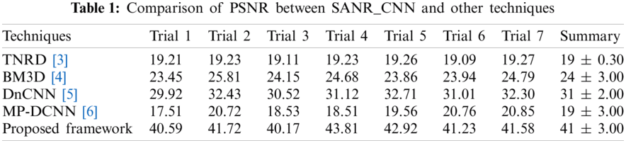
This section describes the various experiments that were conducted to get high-performance efficiency on a similar dataset for MR images used in contrast to other modern techniques. Multiple experiments were conducted to denoise the MR images. The proposed denoising technique reduced Gaussian and Rician errors for MR images. Experimental outcomes verified the high reconstruction quality of various medical images using our proposed model. The experimental outcomes outperformed conventional techniques in terms of PSNR, MSE, and SSIM. Our outcomes demonstrated a substantially increased efficiency and reconstruction accuracy. Our model needed very less execution time for the processing of large datasets. The proposed SANR_CNN model was modeled and executed on Intel i3, 3.2 GHz with 12 GB RAM using a Windows operating system. The proposed SANR_CNN model was compared with the different noise removal TNRD, BM3D, DnCNN and MP-DCNN. The proposed model has depth same as DnCNN approach. The initial metrics are (i) alpha1, alpha2, epsilon, and learning rate that are 0.9, 0.999, 1 * 10−8, and 1 * 10−3 respectively. (ii) The number of epochs is 180 and number of batches set to 226. The learning rate of epochs are 1 * 10−3 to 1 * 10−8.
In the modern era, the need for noiseless high-quality medical images resulted in the immense growth of MR images. Therefore, the demand for an effective technique that can accurately reconstruct high-quality medical images in real-time after compression is huge. Hence, we have presented a CNN model with the sparse representation technique SANR_CNN to ensure high-quality denoised MR images. All the experiments were implemented for the MR images (T1-weighted, T2-weighted and FLAIR). The SANR_CNN model was implemented using a MATLAB library and the Python framework. The entire experiments were conducted under a parallel GPU computing environment using a CUDA computing framework.
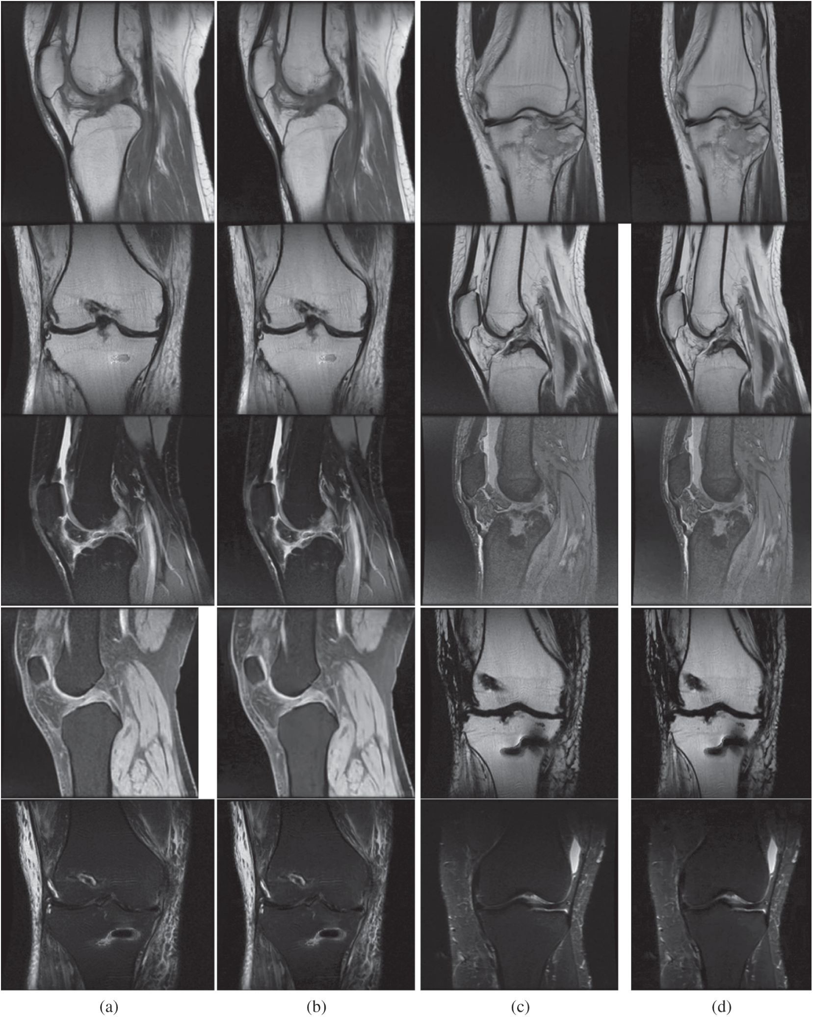
Figure 4: Outcome achieved using the proposed model. Figs. 4a and 4c are medical input images. Similarly, Figs. 4b and 4d are outcomes of the proposed model. The first row represents T1-weighted images, the second row represents FLAIR images and the remaining rows represent T2-weighted images. (a) Input image. (b) Reconstructed image. (c) Input image. (d) Reconstructed image
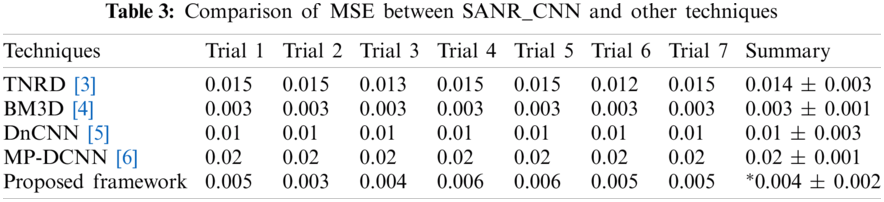
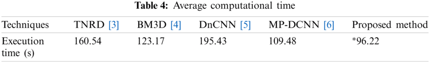
The experiment was conducted in seven trials and a summary was collected. Fig. 4 discusses the outcomes of the medical images. The first and third columns illustrate the input images, and the second and fourth columns illustrate the outcome of the proposed model. The model has experimented on a few MR images such as: T1-weighted MR images represented in the first row, FLAIR MR images in the second row, and T2-weighted MR images represented in the remaining rows. Tab. 1 describes the PSNR, where our proposed model provided an outcome of more than 40 dB for all trails. Tab. 2 provides information regarding the SSIM of the proposed model and compared it with different methods. The proposed model exhibited an SSIM value of 0.87 ± 0.08 which was best among other compared methods. Tab. 3 provides information regarding the MSE, exhibiting that our model gave the least error compared with others. Tab. 4 discusses the computational time required for the overall processing of the image. The proposed model processed with an approximate time of 96 s.
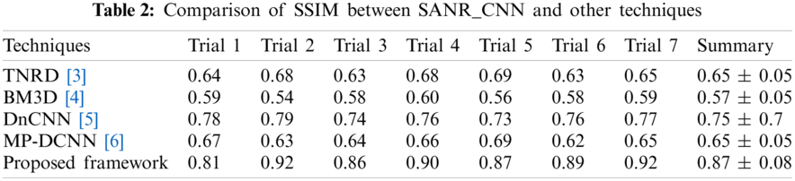
The ease of understanding the illustration of experimental measures used efficiently in our model are represented in Figs. 5–8. Fig. 5 illustrates the SSIM. The proposed model achieved the measure of approximately 0.87, which is the best compared with the measures achieved by other methods. The other methods achieved an approximate average value of 0.65. Method 2 has exhibited the lowest value of 0.57.
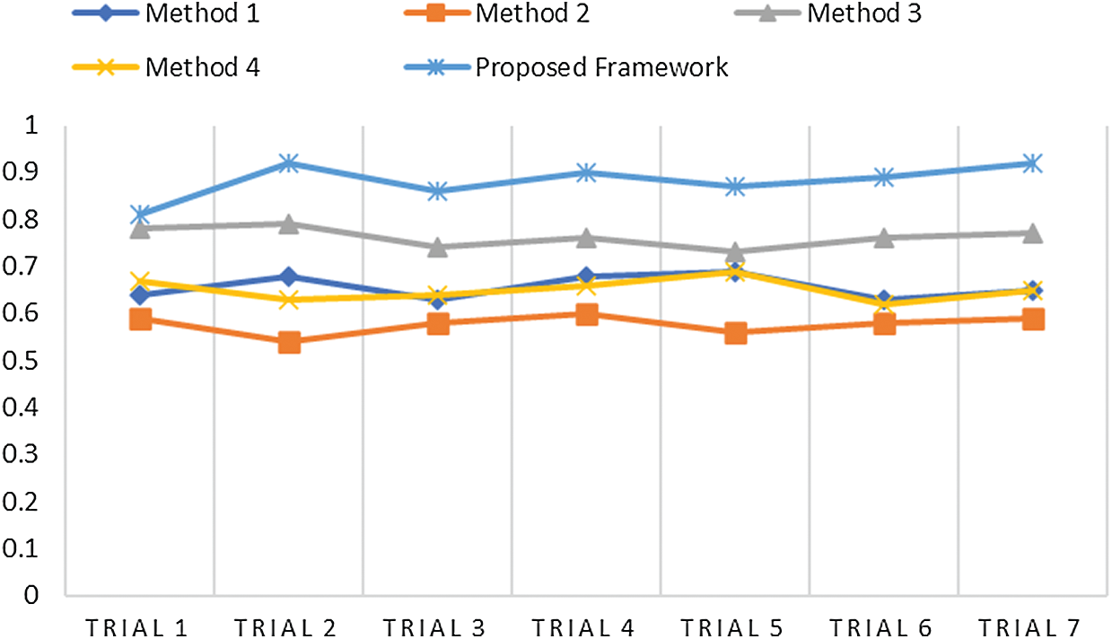
Figure 5: Comparative analysis of SSIM of the proposed method and other techniques
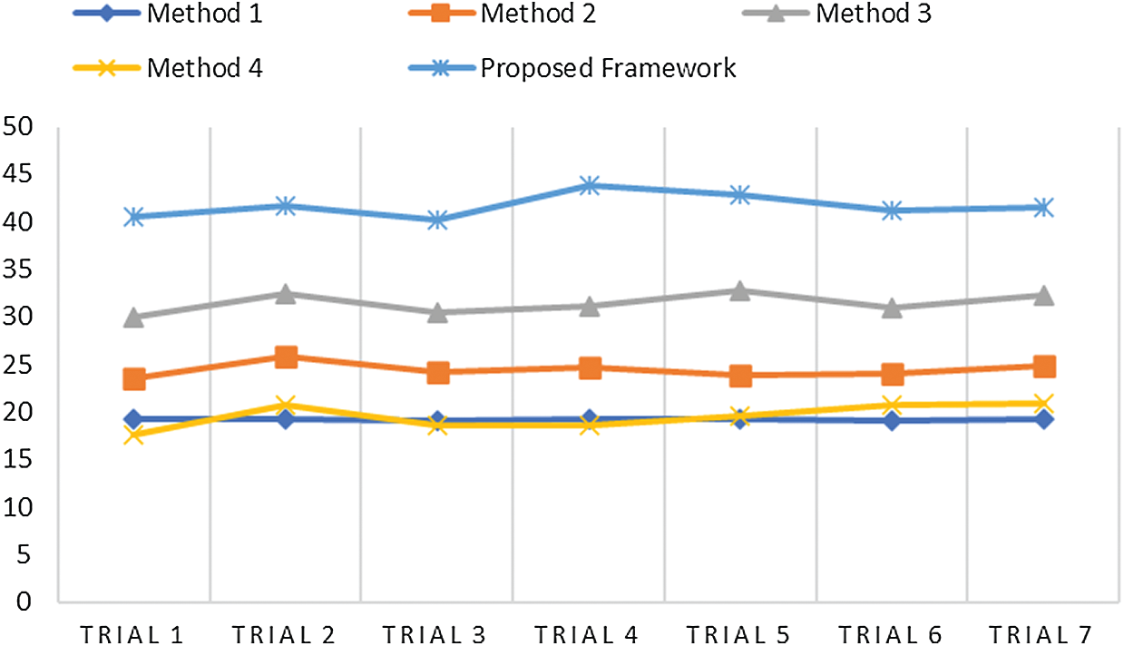
Figure 6: Comparative analysis of PSNR of the proposed method and other techniques
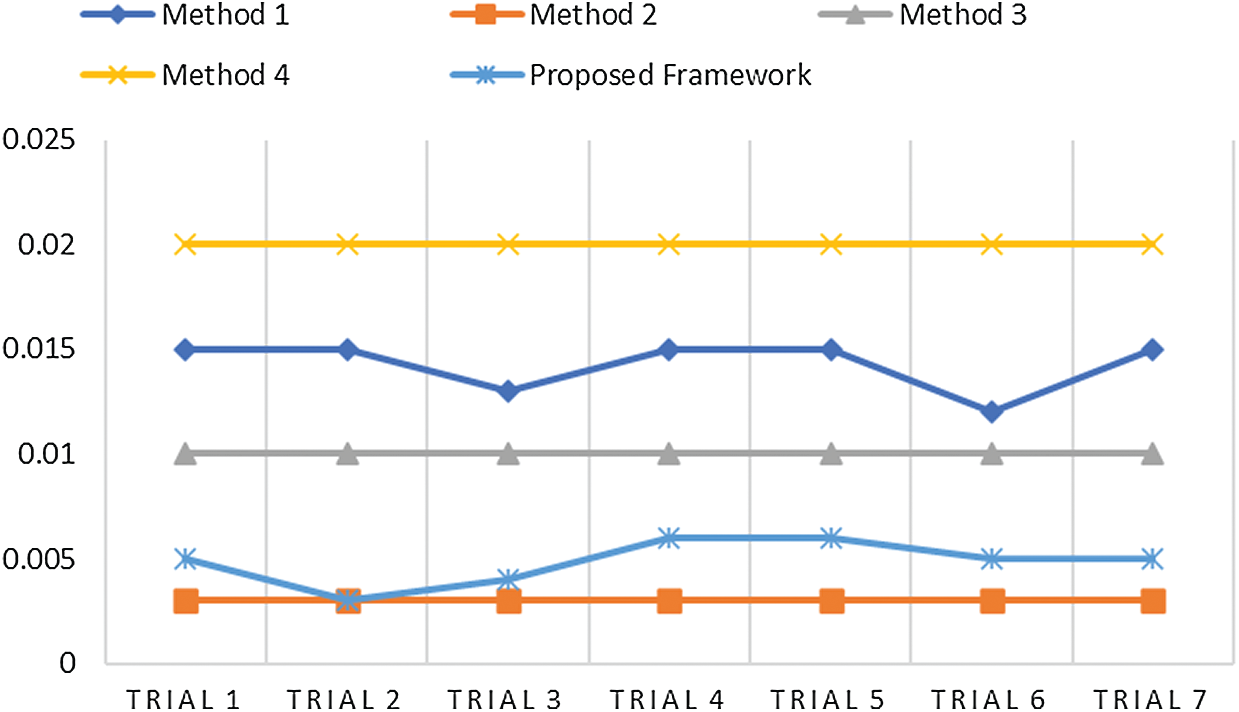
Figure 7: Comparative analysis of MSE and other techniques
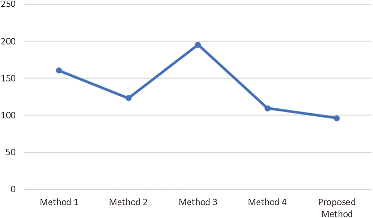
Figure 8: Comparative analysis of average computational time
Fig. 6 illustrates PSNR value, which should always be more, so that noise can be eliminated. Our proposed model achieved an average value of approximately 41 dB; thus, it can eliminate the noise occurred during acquisition in the MR images. Methods 1 and 4 achieved the same outcomes in terms of PSNR. Method 3 gained a higher PSNR value with 31 dB. Fig. 7 illustrates the MSE of all the methods used for analytical comparison with the proposed model. The MSE achieved by our model was approximately 0.004. Fewer errors were found in our model during processing. Fig. 8 illustrates an approximate execution time of 96 s. The other comparative methods demonstrated that Method 4 possessed the value nearest to that of the proposed model.
MRI is a nonradioactive detection method extensively used to inspect biological structures and arrangements of the human physique. However, MR medical image detection is a complex, slow, and bulky procedure. Therefore, we implemented a SANR technique using the CNN architecture (SANR_CNN) for the fast high-quality reconstruction of MR medical images. In our SANR_CNN model, we implemented a dictionary learning algorithm by producing a dictionary while training for the efficient denoising of various types of noises. We used various parameters to define the high quality of our reconstructed MR medical images, namely PSNR and SSIM. The overall results demonstrated that the proposed SANR_CNN model performed considerably much better than other noise removal techniques with respect to PSNR, MSE, and SSIM. Our model produced high PSNR results of 41±3.0 dB, which is considerably higher than those produced by any other algorithm. Additionally, it achieved MSE of 0.004 ± 0.002, which is much lower than that achieved by other noise removal techniques. Similarly, the SSIM outcomes 0.87 ± 0.08 obtained using our model SANR_CNN. These results demonstrate the superiority of our proposed model over a few other techniques.
We would further improve the contrast parameter of reconstructed MRIs with a better hybrid algorithm. In the future along with improvement in processing speed, range of transmission, and carryout performance evaluation considering more diverse datasets and performance metrics.
Author Contribution: All authors contributed to data analysis, writing, and editing the manuscript.
Funding Statement: This research was financially supported in part by the Ministry of Trade, Industry and Energy (MOTIE) and Korea Institute for Advancement of Technology (KIAT) through the International Cooperative R&D program. (Project No. P0016038) and in part by the MSIT (Ministry of Science and ICT), Korea, under the ITRC (Information Technology Research Center) support program (IITP-2021-2016-0-00312) supervised by the IITP (Institute for Information & communications Technology Planning & Evaluation).
Conflicts of Interest: The authors declare that they have no conflicts of interest to report regarding the present study.
1. C. Tian and H. Zhang, “Application of partial differential equation in brain image segmentation and registration,” IEEE Access, vol. 7, pp. 19631–19642, 2019. [Google Scholar]
2. C. Iwendi, S. Khan, J. H. Anajemba, A. K. Bashir and F. Noor, “Realizing an efficient IoMT-assisted patient diet recommendation system through machine learning model,” IEEE Access, vol. 8, pp. 28462–28474, 2020. [Google Scholar]
3. L. Axel, A. Montillo and D. Kim, “Tagged magnetic resonance imaging of the heart: A survey,” Medical Image Analysis, vol. 9, no. 4, pp. 376–393, 2005. [Google Scholar]
4. T. Reddy, G. S. Bhattacharya, P. K. Reddy, S. Hakak, W. Z. Khan et al., “Antlion re-sampling based deep neural network model for classification of imbalanced multimodal stroke dataset,” Multimedia Tools and Applications, 2020. https://doi.org/10.1007/s11042-020-09988-y. [Google Scholar]
5. J. Bates, I. Teh, D. McClymont, P. Kohl, J. E. Schneider et al., “Monte Carlo simulations of diffusion weighted MRI in myocardium: validation and sensitivity analysis,” IEEE Transactions on Medical Imaging, vol. 36, no. 6, pp. 1316–1325, 2017. [Google Scholar]
6. D. Liang, E. V. R. DiBella, R. R. Chen and L. Ying, “k-t ISD: Dynamic cardiac MR imaging using compressed sensing with iterative support detection,” Magnetic Resonance in Medicine, vol. 68, no. 1, pp. 41–53, 2012. [Google Scholar]
7. M. Lustig, D. Donoho and J. M. Pauly, “Sparse MRI: The application of compressed sensing for rapid MR imaging,” Magnetic Resonance in Medicine, vol. 58, no. 6, pp. 1182–1195, 2007. [Google Scholar]
8. Y. Pang and X. Zhang, “Interpolated compressed sensing for 2D multiple slice fast MR imaging,” PLoS One, vol. 8, no. 2, pp. e56098, 2013. [Google Scholar]
9. G. Ramos-Llorden, A. J. den Dekker and J. Sijbers, “Partial discreteness: A novel prior for magnetic resonance image reconstruction,” IEEE Transactions on Medical Imaging, vol. 36, no. 5, pp. 1041–1053, 2017. [Google Scholar]
10. A. K. Seghouane and A. Iqbal, “Sequential dictionary learning from correlated data: Application to fMRI data analysis,” IEEE Transactions on Image Processing, vol. 26, no. 6, pp. 3002–3015, 2017. [Google Scholar]
11. Wenzhe Shi, X. Zhuang, H. Wang, S. Duckett, V. N. Luong et al., “A comprehensive cardiac motion estimation framework using both untagged and 3-D tagged MR images based on nonrigid registration,” IEEE Transactions on Medical Imaging, vol. 31, no. 6, pp. 1263–1275, 2012. [Google Scholar]
12. F. Xu, J. Han, Y. Wang, M. Chen, Y. Chen et al., “Dynamic magnetic resonance imaging via nonconvex low-rank matrix approximation,” IEEE Access, vol. 5, pp. 1958–1966, 2017. [Google Scholar]
13. B. Zhao, J. P. Haldar, A. G. Christodoulou and Z. P. Liang, “Image reconstruction from highly undersampled (k, t) space data with joint partial separability and sparsity constraints,” IEEE Transactions on Medical Imaging, vol. 31, no. 9, pp. 1809–1820, 2012. [Google Scholar]
14. S. Kutia, S. H. Chauhdary, C. Iwendi, L. Liu, W. Yong et al., “Socio-technological factors affecting user's adoption of eHealth functionalities: A case study of China and Ukraine eHealth systems,” IEEE Access, vol. 7, pp. 90777–90788, 2019. [Google Scholar]
15. A. Shanmugam and S. Rukmani Devi, “A fuzzy model for noise estimation in magnetic resonance images,” Innovation and Research in BioMedical Engineering, vol. 41, no. 5, pp. 261–266, 2020. [Google Scholar]
16. V. Magudeeswaran, C. G. Ravichandran and P. Thirumurugan, “Brightness preserving bi-level fuzzy histogram equalization for MRI brain image contrast enhancement,” International Journal of Imaging Systems and Technology, vol. 27, no. 2, pp. 153–161, 2017. [Google Scholar]
17. F. Xiaoyu, L. Qiusheng and S. Baoshun, “Compressed sensing MRI with phase noise disturbance based on adaptive tight frame and total variation,” IEEE Access, vol. 5, pp. 19311–19321, 2017. [Google Scholar]
18. S. Abdullah, O. Arif, M. Bilal Arif and T. Mahmood, “MRI reconstruction from sparse k-space data using low dimensional manifold model,” IEEE Access, vol. 7, pp. 88072–88081, 2019. [Google Scholar]
19. H. Zheng, K. Zeng, D. Guo, J. Ying, Y. Yang et al., “Multi-contrast brain MRI image super-resolution with gradient-guided edge enhancement,” IEEE Access, vol. 6, pp. 57856–57867, 2018. [Google Scholar]
20. X. Zhao, T. Zhang, H. Liu, G. Zhu and X. Zou, “Automatic windowing for MRI with convolutional neural network,” IEEE Access, vol. 7, pp. 68594–68606, 2019. [Google Scholar]
21. X. You, N. Cao, H. Lu, M. Mao and W. Wanga, “Denoising of MR images with rician noise using a wider neural network and noise range division,” Magnetic Resonance Imaging, vol. 64, pp. 154–159, 2019. [Google Scholar]
22. J. Yuan, “MRI denoising via sparse tensors with reweighted regularization,” Applied Mathematical Modelling, vol. 69, pp. 552–562, 2019. [Google Scholar]
23. F. Baselice, G. Ferraioli, V. Pascazio and A. Sorriso, “Denoising of MR images using Kolmogorov-Smirnov distance in a non-local framework,” Magnetic Resonance Imaging, vol. 57, pp. 176–193, 2019. [Google Scholar]
24. H. V. Bhujle and B. H. Vadavadagi, “NLM based magnetic resonance image denoising–A review,” Biomedical Signal Processing and Control, vol. 47, pp. 252–261, 2019. [Google Scholar]
25. J. Chen, W. Yu, J. Tian, L. Chen and Z. Zhou, “Image contrast enhancement using an artificial bee colony algorithm,” Swarm and Evolutionary Computation, vol. 38, pp. 287–294, 2018. [Google Scholar]
26. V. Hanchate and K. Joshi, “MRI denoising using BM3D equipped with noise invalidation denoising technique and VST for improved contrast,” Springer Nature Applied Sciences, vol. 2, no. 2, pp. 234, 2020. [Google Scholar]
27. I. Nagarajan and G. G. Lakshmi Priya, “Removal of noise in MRI images using a block difference-based filtering approach,” International Journal of Imaging Systems and Technology, vol. 30, no. 1, pp. 203–215, 2020. [Google Scholar]
28. I. S. Isa, S. N. Sulaiman, M. Mustapha and N. K. A. Karim, “Automatic contrast enhancement of brain MR images using average intensity replacement based on adaptive histogram equalization (AIR-AHE),” Biocybernetics and Biomedical Engineering, vol. 37, no. 1, pp. 24–34, 2017. [Google Scholar]
29. H. Wang, R. Zheng, F. Dai, Q. Wang and C. Wang, “High-field MR diffusion-weighted image denoising using a joint denoising convolutional neural network,” Journal of Magnetic Resonance Imaging, vol. 50, no. 6, pp. 1937–1947, 2019. [Google Scholar]
30. Y. Chen, Q. Zhao, X. Hu and B. Hu, “Multi-resolution parallel magnetic resonance image reconstruction in mobile computing-based IoT,” IEEE Access, vol. 7, pp. 15623–15633, 2019. [Google Scholar]
31. M. Elhoseny, K. Shankar, S. K. Lakshmanaprabu, A. Maseleno and N. Arunkumar, “Hybrid optimization with cryptography encryption for medical image security in internet of things,” Neural Computing and Applications, vol. 32, no. 15, pp. 10979–10993, 2020. [Google Scholar]
32. P. Lin, D. C. Lyu, F. Chen, S. S. Wang and Y. Tsao, “Multi-style learning with denoising autoencoders for acoustic modeling in the internet of things (IoT),” Computer Speech and Language, vol. 46, pp. 481–495, 2017. [Google Scholar]
33. Y. Chen and T. Pock, “Trainable nonlinear reaction diffusion: A flexible framework for fast and effective image restoration,” IEEE Transactions on Pattern Analysis and Machine Intelligence, vol. 39, no. 6, pp. 1256–1272, 2017. [Google Scholar]
34. K. Dabov, A. Foi, V. Katkovnik and K. Egiazarian, “Image denoising by sparse 3-D transform-domain collaborative filtering,” IEEE Transactions on Image Processing, vol. 16, no. 8, pp. 2080–2095, 2007. [Google Scholar]
35. K. Zhang, W. Zuo, Y. Chen, D. Meng and L. Zhang, “Beyond a gaussian denoiser: residual learning of deep CNN for image denoising,” IEEE Transactions on Image Processing, vol. 26, no. 7, pp. 3142–3155, 2017. [Google Scholar]
36. S. Gai and Z. Bao, “New image denoising algorithm via improved deep convolutional neural network with perceptive loss,” Expert Systems with Applications, vol. 138, pp. 112815, 2019. [Google Scholar]
 | This work is licensed under a Creative Commons Attribution 4.0 International License, which permits unrestricted use, distribution, and reproduction in any medium, provided the original work is properly cited. |