Computers, Materials & Continua DOI:10.32604/cmc.2021.018472
Article

An AW-HARIS Based Automated Segmentation of Human Liver Using CT Images

P. Naga Srinivasu1, Shakeel Ahmed2,*, Abdulaziz Alhumam2, Akash Bhoi Kumar3 and Muhammad Fazal Ijaz4

1Department of Computer Science and Engineering, GITAM Institute of Technology, GITAM Deemed to be University, Visakhapatnam, 530045, India
2Department of Computer Science, College of Computer Sciences and Information Technology, King Faisal University, Al-Ahsa, 31982, Saudi Arabia
3Department of Electrical and Electronics Engineering, Sikkim Manipal Institute of Technology, Sikkim Manipal University, Majitar, 737136, India
4Department of Intelligent Mechatronics Engineering, Sejong University, Seoul, 05006, Korea
*Corresponding Author: Shakeel Ahmed. Email: shakeel@kfu.edu.sa
Received: 10 March 2021; Accepted: 25 April 2021

Abstract: In the digestion of amino acids, carbohydrates, and lipids, as well as protein synthesis from the consumed food, the liver has many diverse responsibilities and functions that are to be performed. Liver disease may impact the hormonal and nutritional balance in the human body. The earlier diagnosis of such critical conditions may help to treat the patient effectively. A computationally efficient AW-HARIS algorithm is used in this paper to perform automated segmentation of CT scan images to identify abnormalities in the human liver. The proposed approach can recognize the abnormalities with better accuracy without training, unlike in supervisory procedures requiring considerable computational efforts for training. In the earlier stages, the CT images are pre-processed through an Adaptive Multiscale Data Condensation Kernel to normalize the underlying noise and enhance the image’s contrast for better segmentation. Then, the preliminary phase’s outcome is being fed as the input for the Anisotropic Weighted–-Heuristic Algorithm for Real-time Image Segmentation algorithm that uses texture-related information, which has resulted in precise outcome with acceptable computational latency when compared to that of its counterparts. It is observed that the proposed approach has outperformed in the majority of the cases with an accuracy of 78%. The smart diagnosis approach would help the medical staff accurately predict the abnormality and disease progression in earlier ailment stages.

Keywords: CT image; automated segmentation; HARIS; anisotropic weighted; social group optimization

1  Introduction

It is well known that medical image processing and computer-aided diagnosis have advanced significantly in recent years. Medical imaging is essential in the process of evolving a plan of action for clinical therapy and surgery. In such a case, analysis is critical for a better interpretation and identification of the ailments from the medical CT, MRI, and PET scan images. By performing the examination and analysis of medical images, various regions and artefacts in the region of interest can be easily identified. This paved the way for research involving the medical image segmentation process to identify abnormalities that would assist in surgical procedure planning and decision-making. Among the various imaging technologies available, MRI imaging is the most predominantly used technology for medical diagnosis as it can represent the various elements and artifacts of internal body parts in the most detailed manner. CT is the most widely used technology alongside MRI technology due to its vast spectral resolution, greater convenience to access, and faster image acquisition time.

To accurately diagnose an acute liver disorder in its early stages and to decide on the best therapeutic option, information pertaining to its precise location and size is required, and CT imaging is the most commonly used technology for identifying such artifacts. It offers detailed anatomical details about the abdomen organs and tissues. The manual process of segmenting the CT Scan images for the abnormality identification is tedious and needs considerable effort. The liver is exceptionally different in concern to the size and the shape of individuals. The acquired CT scan images might have divergent non-liver artifacts, and images might be of low contrast, making disorder identification quite challenging. Additionally, the size, shape, and texture of the affected region vary depending on the severity of the liver disorder. There are plenty of automated approaches used to segmentation the medical CT images classified as semi-automated and automated segmentation approaches [1–3]. The quality of the segmentation depends on the preciseness of the proposed model and the features that are selected for the segmentation. The outcomes of either of those approaches would be almost identical, but the automated segmentation techniques outcome is more accurate on practical implementation.

There are various supervised and semi-supervised approaches that are used in automated segmentation of the CT Scan images. Supervisory models like Deep learning-based approaches (DL) [4,5] and convolutional neural network (CNN) [6,7] need tremendous training for better precision of outcome. The quality of the resultant outcome is directly proportional to the size of the training set. The outcome of the approaches mentioned above is more suitable for medical-related image analysis, as they are highly accurate and precise. The main issue with the approaches as mentioned earlier is that the availability of the training set for identification of the lesion. Moreover, with the most recently discovered form of any disorder, previously acquired data for training the algorithm may be inaccessible, resulting in an ineffective automated segmentation of the images.

Particle Swarm Optimization [8,9] based CT/MR image segmentation is a metaheuristic in nature. It can effectively handle the data without any prior knowledge about the context and handle ample search space efficiently. It is being observed that the suggested approach is comparatively easy to implement and strong enough to address the issue of heterogeneous regions in the image and performs better in contrast to the conventional Genetic Algorithm approach. Support vector machine (SVM) [10] is considered one of the best approaches for automated segmentation of the CT/MR image through a classification mechanism that can knob the unstructured images and high dimensional data efficiently with a comparatively lesser storage requirement. However, SVM has the limitation of training the machine with a large amount of data in order to achieve decent performance, which requires additional computing time and storage space for the training collection that results in additional computational efforts. Additionally, locating the case-specific training data is a tedious task.

Convolutional neural networks [11,12] based models for brain and liver image segmentation have proven to be most accurate by researchers. CNN models are designed to handle the high dimensional data by recognizing the features and the translation invariance that are essential for automated segmentation. Automated CT image segmentation based on Single-Block Linear Detection (SBLD) [13] is reasonably accurate in identifying the abnormalities and requires few iterations to reach the optimal level of segmentation, resulting in less computational efforts. But the SBLD model largely relays on the initial parameters for the segmentation.

Deep learning [14] based liver MR image segmentation is considered efficient in handling unstructured and ambiguous data. It doesn’t need the labeling of the data. However, the deep learning models are complex to design and they need a large training set for an acceptable level of performance. In some cases, the large amount of training data may cause the model to overfit. The Active Contour model [15] is an automated segmentation framework that works by considering the boundaries and the curvature of the target for the region outline contour. The Active Contour model is an adaptive searching model that needs minimal computational efforts. The process of identify and elucidate the features would be the most challenging job of fitting it into a problem-centric mechanism. This particular approach is not always suitable for the image with huge explore domain space.

The objective of the paper is to mechanize a systematic procedure that can automatically diagnose human liver abnormalities from CT image through a self-regulated segmentation model. Through conventional strategies like k-means, Fuzzy C-Means, Seed Region Growing, and Graph-cuts-based semi-automated approaches for the segmentation, there are considerable limitations that are susceptible to misinterpretation of the normal tissues as an abnormality, and deciding the initial parameters is a challenging task. To address the challenges of semi-automated approaches, fully robotic approaches have been implemented, including the Genetic Algorithm, Deep Learning, and Neural Network. But all the aforementioned automated approaches need considerable computational efforts and meticulous training for a better resultant outcome. We have proposed a computationally efficient method and robust mechanism, namely the AW-HARIS algorithm for automated segmentation of the CT image that assists in ease of abnormality identification, on evaluating the proposed approach through various performance evaluation metrics the outcome is reasonable with minimal computational efforts.

The complete paper is being organized along these lines; the first portion of the paper deals with the introduction and various existing mechanism and their challenges. The following section is about the proposed algorithm that includes the Adaptive Multiscale Data Condensation Kernel-based de-noising approach, AW-HARIS-based segmentation approach followed by the dataset used, and the experimental setup are presented in this section. The third section of the paper presents the experimental results and discussions, and the performance analysis through various metrics has been furnished. Finally, the paper concludes with a conclusion and future scope.

2  Adaptive Multiscale Data Condensation (AMDC) Kernel

Adaptive Multiscale Data Condensation [16,17] is a robust mechanism used in Noise elimination and image magnification in the proposed model. The ADMC method pivots the portrayal of the information related to image pixels’ consistency with the solidity of distribution of solitary search space, i.e., the kernel’s original proportions. The magnitudes’ dependability would vary from every window that upshots a difference in the noisy pixel parameters. The architecture diagram of the AMDC kernel is represented in Fig. 1, with all the necessary components incorporated.

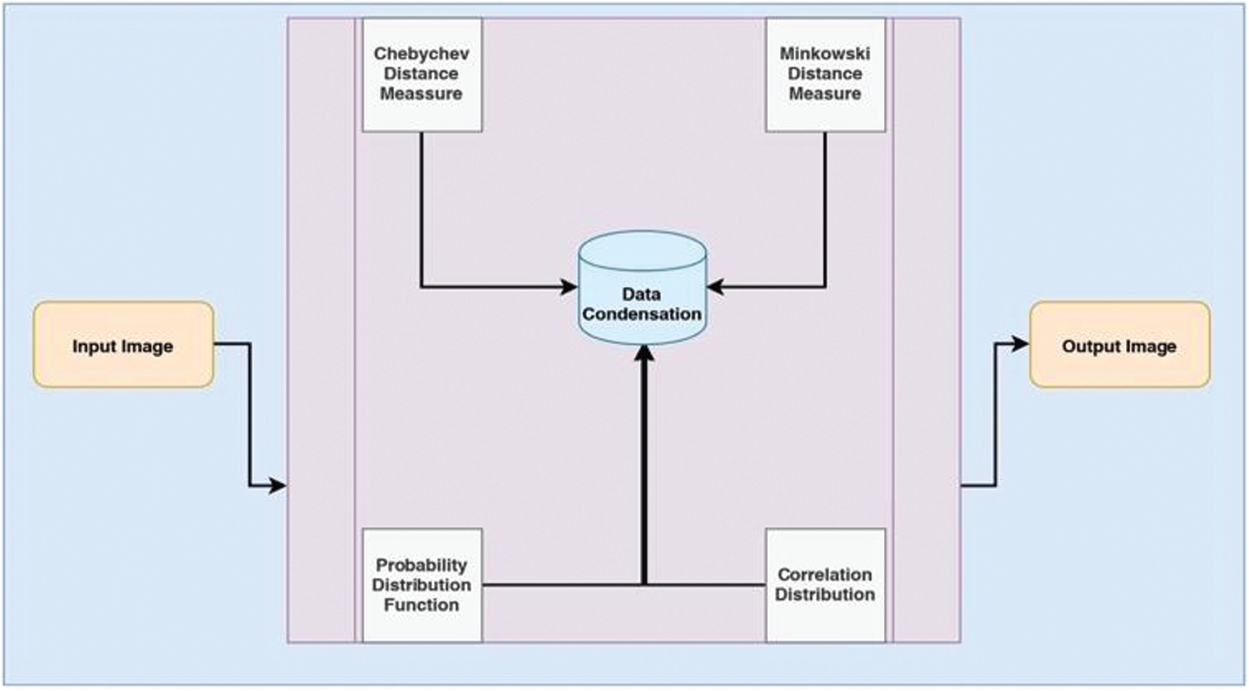
Figure 1: Architectural diagram of the AMDC kernel

The fewer corresponding points concerning the approximated seed points are being recognized. A few of them that are not part of the search space are being ignored through the evaluation process’s classification parameters. The seed points that are being categorized and that are probably the part of the k nearest neighborhood are presumed to be identified with a set of M points that are the part of the search domain with an approximated radius r concerning the point p in an Md dimensional search space. Now the formula for the hyperplane is identified as shown in Eq. (1)

Hplan(r,p)={x∣dist(x,p)≤r,x∈X}(1)

From the above equation, dist(x,p) determines the distance measure among the point x and the centroid p of the hyperplane, And the Lebesgue measurement in the hyperplane is approximated using Lm(x,p). It is determined through the set {xs: s = 1, 2, 3,…, n, n→∞} and the distance is calculated through dist(s,p) for each sth point to the corresponding the pth neighborhood point. The probability distribution function is represented through Dp is used to direct by the asymptotically robust formula

Dp=pn×1fr(s,p)(2)

Eq. (2) can be used with a 2D CT image whose size is determined by Ii×j and TP=i×j, representing the complete number of pixels in the entire image. The proposed de-noising mechanism will recognize only the hidden crucial points assumed to be the seed points by performing the above task. So, the dissimilarity between the two predetermined seed points differs from the approximated probability density function among the identified seed points. The approach that assesses the distance measure among each approximated point using the Minkowski metric [18] is stated through Eq. (3) as follows

distm=(∑i=1N|pai-pbi|z)z(3)

when z=1, that is like a city-block distance measure [19], and when the value of z=2 it resembles to be like a Euclidean distance measure, and when the value of z=∞ the value of the Chebychev distance [20], is assessed through the Eq. (4) as follow

distmsr=maxi|xai-xbi|(4)

The association between the two seed points (m,n) is assessed using the formula in Eq. (5)

a(m,n)=e-α×distmnrWhere α=-(ln0.5)dist>0(5)

The value of the arbitrary variable α is determined as above, where ln denotes the approximated mean distance measure between the two corresponding seed points available distance matrix.

3  AW Based HARIS Approach for CT Image Segmentation

In this paper, an enhanced version of the Heuristic approach for real-time segmentation using the Anisotropic Weighted module improves the HARIS [21] algorithm’s performance. The improved version of the HARIS is organized efficiently compared to the conventional HARIS algorithm and its equivalents. The AW-HARIS works with multiple objective functions to identify a random number of segments and assign the membership function pixels. And further, the segments are refined through the other objective process, and it continues until it reaches the best possible number of segments that elaborate every minute object in the image. The proposed mechanism would identify the best possible number of inception segments through the elbow methods, whose equation is stated in Eq. (6)

is=∑si=1n∑pi∈ti∥pi-centroidi∥(6)

From Eq. (6), the variable pi designates the pixels in the ith segment of the image, and the variable centroidi designates the centroid of the ith segment in the image. The entire equation is identified through the variable that approximates the initial number of segments for the segmentation. The value of n is assumed to approximately equivalent to 24 from the previous studies. However, the 24 may not be the same value though out the iterations, and it may not be the final value for evaluation. Si designates the range of image regions that are assumed as segments in the range 1 ton. The variable Centroidi whose value is evaluated from the formulating that is stated by Mac Queen model [21]. The algorithm is being modified such that it is suitable to address the challenge. The formula to identify the centroid is stated below

centroidi=∑pix=1n∑segmnt=1sαpix,segmnt β(xpix,centroidsegmnt)(7)

In Eq. (7), the variable centroidsegmnt designates the appropriate pixel that can be considered the segment centroid, concerning the segment identified through the variable segmnt. And the variable αpix,segmnt from the equation designated the likelihood or can also be called the pixel membership in concern to the segment xpix, The variable that designated the xth pixel in the segmented and the variable centroidsegmnt that designated the centoidth center in the given segment whose value lies between 1 to s. β(xpix,centroidsegmnt) is the distance measures that are being used in estimating the membership. The distance measure is estimated using the Mahalanobis distance mechanism [22], which estimates the data centroid’s closeness a significant local maximum point. The distance metric is to be considered as standard deviation concerning a point. If the approximated distance measure is too large, then the pixel can be accredited to an alternative centroid whose estimated distance is smaller.

The distance estimation is concerned with the centroid pixel intensity rather than considering the coordinates’ distance, as we generally do it in the Euclidean distance approach. The Mahalanobis distance estimates the mean of the feature vector that gives the average of the pixel intensities in the inception population in the image that is approximated image kernel using Eq. (8)

μm={μp1(m)μp2(m)μp3(m)…μpi(m)}={∑i=1imIp1∑i=2imIp2…∑i=mimIpm}(8)

In Eq. (8), the variable m designates various classes of pixel intensities that are considered the inception population. The pixels in each segment are concerned to the image segment whose centroid is identified through the Eqs. (9) and (10)

Segm=∑i=1m(Iim-μm)(Iim-μm)T(9)

WhereIim=(Ii=1(m),Ii=2(m),Ii=3(m)…Ii=m(m))T(10)

The Mahalanobis distance to unexploited pixels identified by I to allot it to the pixel segment segmnt can be assessed using the following Eq. (11)

n2(I,pm)=(I-μ(m))TINi-1(I-μ(m))(11)

In Eq. (11), the variable INi-1 defines the inverse matrix, which is assessed from the unbiased evaluated covariance matrix as shown in Eq. (12)

INi-1=(xi-1)Segm-1(12)

Once the distance is evaluated and the likelihood or the degree of belongingness by using the Mahalanobis distance measure as mentioned above distance mechanism, all the pixels are allotted to the appropriate segment. And the assessed membership is being used later in the objective Function-I of the proposed mechanism.

3.1 AW-HARIS Algorithm’s First Objective Function

In the proposed mechanism, multiple objective functions are extensively used throughout the segmentation process that approximate the regions’ optimal number in the assumed CT image. That so crucial that the segmentation will not be either over-fitted or under-fitted. It is segmented so that every minute object is being highlighted clearly in the segmented image. The proposed approach would consider the Anisotropic Weighted (AW) module [23] has exhibited a better optimal solution while approximating the suitable number of segments. Once the regions are decided and the centroids are identified, the pixels are being allotted to the corresponding pixels based on the membership value that is being estimated that is being determined through the Eq. (13)

ceni=1pixsi(pixi=12+pixi=22+…+pixi=n2)1pixsi(pixi=1+pixi=2+…+pixi=n)(13)

In the above equation, the variable ceni is the contra harmonic mean of the pixel intensities that are the part of the image segment. The variable i designates the approximate number of segments between 1 and the N. The value of the ceni is upgraded in every iteration and the variable pixsi designates all the pixels completely in the corresponding segment i. All the pixel intensities in the segment are being assessed to identify the optimal pixel that will be the centroid with a minimal distinction between the present iteration and which is being performed in each iteration.

The standard deviation identified using the variable σ that is evaluated in concern to Segi That denotes the ith segment in the image. The pixels are allotted based on the value of the variableGThrsld that designated the global threshold generally whose value lies between .3 and .6 that is determined by experimental studies over the previous observations presented through Eq. (14)

(σ=|Segi-Intensity of pixelpi|)≤GT(14)

The objective function that is being used to estimate of the likeliness of pixels to be the part of the segment and the pixels are being allotted based on the value of the elucidated distance.

Objfun=Aw×{(α×sppixsegi)+(β×totcentrn)}(15)

In Eq. (15), the arbitrary variables α and β are very significant that are considered to be the deciding factors that control the proposed algorithm’s overall accuracy and efficiency. The equation to determine the value of inter-class variance is identified by α from the Eq. (16). The value of intra-class correlation is identified through the variable β from the Eq. (17). And the sum of all pixels is determined by the variable Sp. The variable pixsegi determines the total number of pixels that are part of the segment i the range lies between 1 to n. The variable totcent would be used to identify the total number of segment centroids in the image. The variable rn designates the total number of pixels in the region r.

α=σpix2(σpix2+σe22)(16)

β=∑si=0nωi(t)σi2(t)(17)

The arbitrary variable α represents the inter-class variance is formulated through the Eq. (16) that is the intra-class coefficient that determines the closeness of pixels that are the part of the same segment that holds a special significance in deciding the accuracy of the approximations performed to form the segments. The arbitrary variable β controls the inter-class variance concerning the centroid of the segments based on thresholding. However, the main inspiration behind estimating the values of arbitrary variables α and β is to minimize the intra-class variance and maximize the inter-class variance.

Now for every pixel centroid identified through the variable totcent in the original CT image identified by I, the neighborhood is being identified through the variable Np as Ix(Ix∈Np). Initially, the values of the variables Ix that represents the grey mean square value outlined in the Gaussian kernel function’s kernel space and the neighborhood variable Np is being assessed. The value of the Anisotropic Weighted is being assessed through the outlined value of the grey mean square.

Where the variable Me be the value of the Ix in the neighborhood Np of the corresponding pixel p to another point Np is determined using the Eq. (18)

Me=[∑ x′∈Np\x(gx′-gx)2np-1](18)

In the above Eq. (18), the variable gx′ and gx represents the grey value of the neighborhood pixels points Ix and np respectively. The mean square error Me the outlined value that can be assessed in concern with mean square kernel spaces. The outlines value of the Me is determined through Ø as stated below

∅=exp[-(Me-∑ x∈NpMenp)](19)

Based on the Eqs. (18) and (19) is used to determine the Anisotropic Weight as follows in Eq. (20)

Aw=∅∑x ∈Np∅(20)

Now the number of segments is to be increased or to be decreased concerning the fitness value. The value of the fitness is assessed by Eqs. (21) and (22)

fit(pixi)=1+abs(Obj(f))if fit(pixi)<0segments needed to be added(21)

fit(pixi)=11+obj(f)if fit(pixi)>0segments needed to be reduced(22)

The number of segments in the proposed approach would keep on changing in each iteration that would keep changing in concern to the fitness of pixel to be the part of the segment and also based on the values of the inter-class variance and intra-class correlation that are computed through the variables α and β.

3.2 AW-HARIS Algorithm Second Objective Function

The later objective function of the proposed mechanism is to judge the most appropriate point that can be used as the centroid of the segment. All the pixels will be assigned to the centroid based on the criteria discussed in the proposed mechanism’s first objective function. All the centroid (center) are picked in coherence with the global best so that the recognized point would be the fittest among all the points in the segment. However, throughout the segmentation and refinement process in every iteration of the proposed algorithm, the corresponding segments’ centroids are updated concerning the predetermined objective function. The pixels would be allotted to the segments according to the membership value that has been computed. In every iteration throughout the process, the values of the arbitrary variables α and β are assessed that would judge whether the segments are to be increased or not. The objective function of the proposed algorithm is stated below in Eq. (23)

cents=rand(0,1)× fit_cents-1+ rand(0,1)×(G_Bestcentfit-fit_cents-1)(23)

In Eq. (23), the function rand( ) would randomly choose a value between the 0 and 1 and the variable fit_cents-1 Designates the corresponding centroid’s fitness concerning the global best in the earlier iteration and the variable G_Bestcent_fit designates the centroid’s fitness value that is assumed to be the global best solution that bears the maximum fitness value among the rest of the centroid in the image. Always the new centroid is picked concerning the global best seed points in the image.

3.3 Removing Unwanted Artifacts from CT Image

The unwanted regions in the CT scan images that include the bone structures and the fat accumulation around the liver region are discarded for precise identification of the abnormal region from the abdominal CT scan image. Removing unwanted artifacts from the CT scan image is done through a sequence of image processing operations that include thresholding and morphological operations. The bit map generation’s threshold estimation process is done through the adaptive Otsu thresholding [24]. Then the morphological opening and closing operations are being performed over the bit map image to implement the approximated threshold value.

3.4 Adaptive Otsu Thresholding

The adaptive Otsu thresholding is used to work with smaller regions with a similar property efficiently. The bitmap image that is generated will be precise in the process of discarding the non-essential regions from the CT scan image. OTSU thresholding assesses the uncertainty of the gray level variance to find the threshold. Based on the pixel intensity values, it classifies them into the liver region and Non-essential region. As part of identifying the optimal threshold value, it performs a set of actions that include probabilistic approximation and means of the liver region’s grey level intensity value and non-liver region, assessing the inter-class, intra-class, between-class variance, and picking the optimal threshold.

The grey level intensities of the image f(i,j) range between [0, 1,…, m −1], the optimal threshold value ot that lies between [0≤ot≤m-1]. The probabilities of the liver and non-liver region are approximated as follows in Eqs. (24) and (25)

plr=∑x=0otpx(24)

pnlr=∑x=otm-1px(25)

where plr in the Eq. (24) is the probability of the pixels in the liver region, pnlr in the Eq. (25) is the probability of the pixels in the non-liver region. px is the ratio of a group of pixels gx of the grey level intensity x among the entire intensity range. The occurrence probability of the particular grey level intensity is being approximated through Eq. (26)

px=gxg(26)

The mean of the greyscale intensity values of the liver region is identified through mlr and non-liver region are identified through the mnlr. The same has been presented in the Eqs. (27) and (28) presented below

mlr=∑x=0otxpxplr(27)

mnlr=∑x=ot+1m-1xpxpnlr(28)

The interclass variance that is identified through σinter that is presented in the Eq. (29) and the intraclass variance that is identified through σintra that is presented in the Eq. (30) that are stated below

σintra2=plrσlr2+pnlrσnlr2(29)

σinter2=plr(mlr-mavg)2+pnlr(mnlr-mavg)2(30)

σtot2=∑x=0m-1(x-mavg)2px(31)

The Eq. (31) represents the total variance among the pixels in the CT scan image. The mavg is the mean of the average of the pixel intensities determined through the following Eq. (32)

mavg=∑x=0m-1xpx(32)

The optimal threshold is approximated through the Eq. (33) that is stated below

σt2=[mavgplr(t)-mlr(t)]2plr(t)[1-plr(t)](33)

Based on the approximated threshold, the bitmap image is generated. All the pixel intensities above the approximated threshold are set to white, and the rest of the pixels are set to black in the image. The binarization is done through the Eq. (34)

if pint≥σt2setpint=1elsepint<σt2then setpint=0(34)

3.5 Image Morphological Operations

The bitmap image generated from the approximated threshold value and the bitmap image is considered the kernel for performing the morphological operations. A close morphological procedure is carried out by performing a dilation trail via erosion to fill out the gaps in the area of interest by smoothing the surface using the square modeling feature STREL, taking into account and filling up the voxel of all the 8 neighboring pixels. Upon filling out the holes, the resultant reference kernel overlaid over the original image and the morphological opening procedure, implying that the bitmap’s image is the attaching feature. A close morphological operation is performed to remove the non-liver region from the CT scan image. The morphological open and close are the compound operations that are performed through dilation and erosion operators.

Morphological Opening:

A morphological opening operation is performed to eliminate the thin protrusions of the input image, and the opening operation includes erosion followed by the dilation process. The Eq. (35) represents the morphological opening operation

(I∘k∘)(i,j)=((I⊖k∘)⊕k∘)(i,j)(35)

Morphological Closing:

A morphological closing operation is performed to fill out the holes by smoothening the regions’ surface in the image and merging the narrow gaps among the image regions. The Eq. (36) represents the morphological closing operation

(I⋅k⋅)(i,j)=((I⊕k⋅)⊖k⋅)(i,j)(36)

The images in Fig. 2 present the outcome of the proposed approach for removing the non-liver artifacts from the image. On removing the non-liver artifacts from the CT scan image, assessing the affected region would be easy. IT also enhances the approximated outcomes accuracy in determining the irregularity’s impact. Moreover, the anomaly is being recognized based on the intensity at the particular impacted region. The non-liver artifacts may sometimes lead to the misinterpretation of the non-tumorous region as the tumorous region. And this phase is considered to be one of the pre-processing stages in approximating the damaged region.

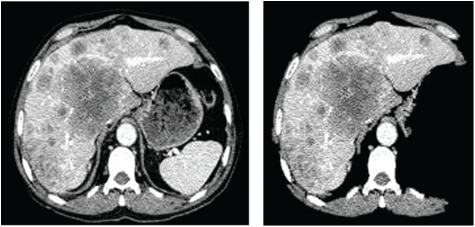
Figure 2: The outcome image on removing the non-liver artifacts

3.6 Dataset

The experimental study images are acquired from the online repository. The Cancer Imaging Archive-LIHC data set version 3, released in March 2017, is a part of The Cancer Genome Atlas (TCGA) The dataset consists of data related to 97 homo sapiens collected over 1,25,397 images in 237 studies [25]. The experimentation is performed over 75 anatomical Liver CT Modality images that are accessed through the OHIF. The dataset is associated with the ground facts for assessing the proposed approach by performing the auto segmentation over the OHIF viewer TCIA Alpha. The results are obtained correlated with the results obtained in the OHIF viewer. The CT images acquired from the open-source data Liver Tumor Segmentation Challenge (LiTS) from MICCAI 2017 [26] are downloaded from the experimental study’s repository to examine against the ground facts. The comparative analysis of the proposed model is done against the available ground facts.

3.7 Experimental Setup

The experimentation is performed in the environment as follows: The machine CPU is an Intel Core I3-3240 processor that works with a fundamental frequency of 3.33 GHz Quad-Core technology. The hard disk is 500 GB, and RAM is 8 GB installed with the Windows 7 operating system’s ultimate version. The experimental setup is run over the MATLAB R2017b using the image processing toolbox. In pre-processing, various built-in methods are used by importing the libraries that include Image Type Conversion, Image Batch Processing, Image registration, Block Processing, Image Region Analyzer as part of the proposed implementation model.

4  Experimental Results and Discussion

The automated segmentation of the Liver CT images of various patient samples acquired from the open-source repositories like the National Cancer Institute, India, and SMIR of multiple sizes is being segmented through the Anisotropic Weighted-HARIS algorithm. The efficiency and the accuracy of the proposed AW-HARIS are being scrutinized in concern with its counterparts like traditional HARIS, Single Block Linear Detection (SBLD), and twin centric GA with Social Group Optimization (SGO) [17]. The performance of the approaches mentioned above is being assessed through various metrics like sensitivity, Specificity, Jaccard Similarity index, and the Matthews Correlation Coefficient from the examined value of True Positive, True Negative, and the False Positive, False Negative that is determined from several successful executions. The acquired images are initially pre-processed in the proposed model through the Adaptive Multiscale Data Condensation (AMDC) Kernel-based approach. The quality of the resultant outcome of the proposed model relies on the quality of the image. The pre-processed image quality is being assessed through the metrics like PSNR, MSE, RMSE, IQI against the images of sizes 256×256 and 512×512.

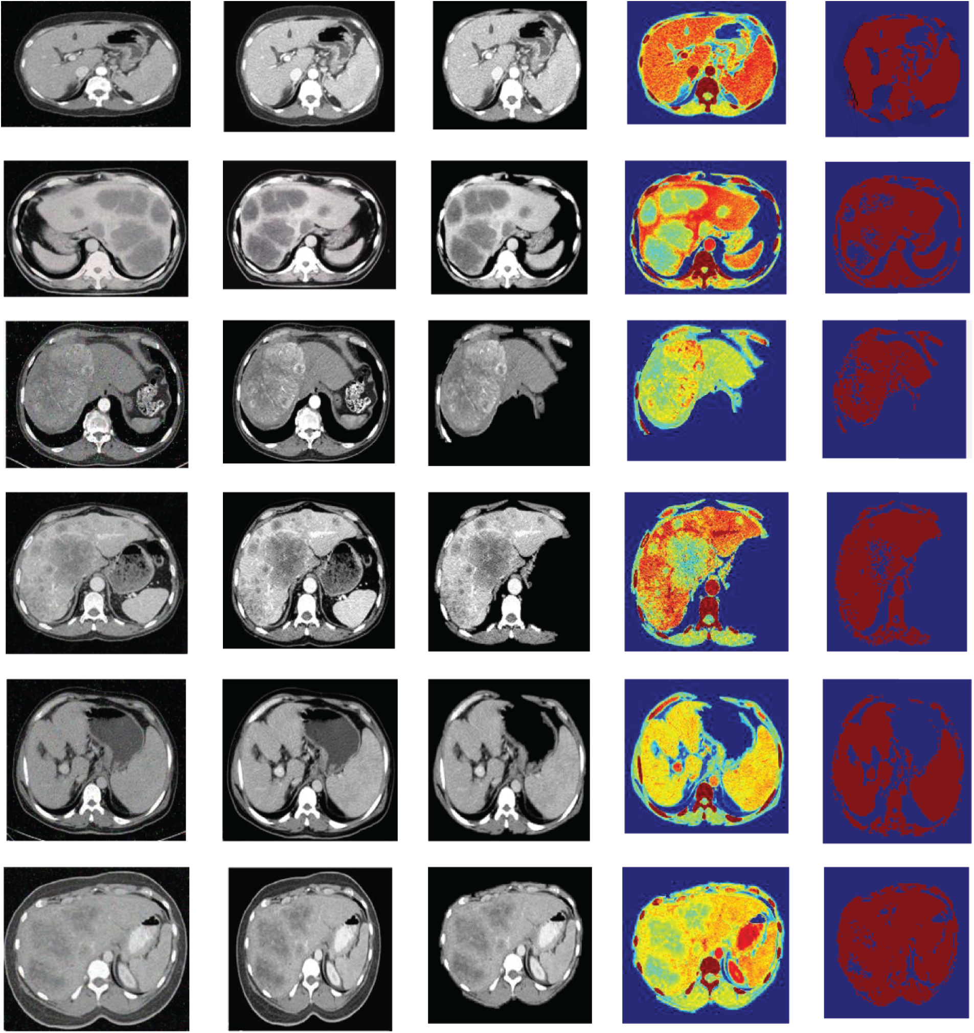
Figure 3: The resultant outcomes of the proposed AW-HARIS approach

In Fig. 3, the leftmost image is the original CT image acquired from the equipment, and the second image from the left represents the de-noise and contrast-enhanced image. The third image is the stripped image for removing the unwanted abdominal tissues. The image next to it represents the segmented image on applying the color-map to the resultant image. The final image is the segmented image with a threshold value of 75. The resulting segmented image is more pleasing when the threshold is appropriately chosen. The color-map is being generated based on the intensities of the underlying tissue are at various grey-level values. The colors-mapping with different grey-level intensities for the segmented image for ease of identification of the abnormal region, the region this is affected is highlighted in the pale green color. As the colormap is applied over the pixel intensity ranges, the neighboring pixels share almost the same color. The actual region of interest can be recognized easily by using the thresholding over the resultant image.

It can be observed from the Tabs. 1 and 2, the performance of the Adaptive Multiscale Data Condensation Kernel is promising. The value of the Peak Signal to noise ratio is increasing with decreased noise variance. The root means square error value has reasonably reduced with an increase in the noise. The IQI value is almost close to the referred high-quality image. It is observed that the AMDC kernel’s performance is more accurate for smaller size CT images over the larger size CT image. The proposed AW-HARIS approach’s performance is being evaluated through metrics like Sensitivity (SEN), Specificity (SPE), Accuracy (AUC), Jaccard Correlation Coefficient (JCI), and Matthews Correlation Coefficient (MCC).

In the experimental studies, the proposed approach is reasonably fair with minimal computation time. However, it takes quite more time than the traditional HARIS algorithm due to assessing the Anisotropic Weight for the pixel assignment. Still, the accuracy is comparatively much better than the HARIS. The experimental values of the proposed model from Tab. 3, that is reasonably good for all the considered parameters. Twin Centric Genetic algorithm-based approach is also an enhanced version of the traditional Genetic algorithm that would allow rigors in moving towards the solution, resultantly that would consume an optimal amount of time in converging towards the best possible number of segments, and to improvise the performance of it, the SG has been incorporated the proposed AW-HARIS yet is computationally feasible with the exact results that can be observed from the experimentation of the proposed approach. The mean execution time automated segmentation of the CT image of size 256×256 is identified as 2.124 s. The CT image of size 512×512 is identified as 3.218 s that involve the images pre-processing through the AMDC filter.

5  Conclusions and Future Scope

It is observed from the practical implementation of the proposed AW-HARIS approach that the resultant outcome is outperforming when validated against ground facts. The proposed method needs a very minimal computational effort than supervisory approaches like CNN, RNN, which needs training, requiring meticulous efforts that would consume more computational resources. The availability of training data is also a challenging task in many cases. In such a context, the proposed approach is technically feasible in identifying the abnormality with its multi-objective function that refines the resultant segmented image over multiple iterations to an adequate level. Every minute region is being focused on appropriately. It incorporates the anisotropic weight that can precisely assign the pixels to the appropriate segment by considering the correlation between the pixel and the segment centroid would significantly impact the segmentation’s accuracy and converges faster towards the solution.

The suggested heuristic approach through the anisotropic weight is reasonably fair in segmenting the CT images. However, it was incredibly challenging when working with original CT images caused due to the suppressed contrast levels that would be burdensome for recognizing the smaller regions from the CT image. This is one of the aspects in which more research can be done. And while working especially with liver CT images, there are many unwanted surrounded regions whose texture appears to be brighter and identical to the damaged region’s texture. Hence it is advisable to discard the non-liver tissues well before the actual segmentation begins so that the algorithm can precisely identify the tumor region.

Funding Statement: The authors have not received any specific funding for this study. This pursuit is a part of their scholarly endeavors.

Conflicts of Interest: The authors declare that they have no conflicts of interest to report regarding the present study.

References

 1.  M. Rela, N. R. Suryakari and P. R. Reddy, “Liver tumor segmentation and classification: A systematic review,” in IEEE-HYDCON, Hyderabad, India, IEEE Conference Proceedings, pp. 1–6, 2020. [Google Scholar]

 2.  P. V. Nayantara, S. Kamath, K. N. Manjunath and K. V. Rajagopal, “Computer-aided diagnosis of liver lesions using CT images: A systematic review,” Computers in Biology and Medicine, vol. 127, pp. 104035, 2020. [Google Scholar]

 3.  P. R. Ros, “Imaging of diffuse and inflammatory liver disease,” In: J. Hodler, R. A. Kubik-Huch, and G. K. von Schulthess, (Eds.) Diseases of the Abdomen and Pelvis 2018–2021: Diagnostic Imaging–IDKD Book chapter 22, Cham: Springer, 2018. [Google Scholar]

 4.  J. G. SivaSai, P. N. Srinivasu, M. N. Sindhuri, K. Rohith and S. Deepika, “An automated segmentation of brain MR image through fuzzy recurrent neural network,” Studies in Computational Intelligence, vol. 903, pp. 163–179, 2021. [Google Scholar]

 5.  P. N. Srinivasu, J. G. SivaSai, M. F. Ijaz, A. K. Bhoi, W. Kim et al., “Classification of skin disease using deep learning neural networks with mobileNet V2 and LSTM,” Sensors, Vol. 21, no. 8, pp. 2852, 2021. [Google Scholar]

 6.  A. S. Parihar, “A study on brain tumor segmentation using convolution neural network,” in Int. Conf. on Inventive Computing and Informatics, Coimbatore, IEEE Conference Proceedings, pp. 198–201, 2017. [Google Scholar]

 7.  Y. Wang, Z. Sun, C. Liu and W. P. J. Zhang, “MRI image segmentation by fully convolutional networks,” in IEEE Int. Conf. on Mechatronics and Automation, Harbin, pp. 1697–1702, 2016. [Google Scholar]

 8.  P. Naga Srinivasu, G. Srinivas, T. Srinivas Rao and V. E. Balas, “A novel approach for assessing the damaged region in MRI through improvised GA and SGO,” International Journal of Advanced Intelligence Paradigms, (In-Press). https://www.inderscience.com/info/ingeneral/forthcoming.php?jcode=ijaip. [Google Scholar]

 9.  A. Abder-Rahman, C. Micael, A. Ahmed and H. A. Ella, “Particle swarm optimization based fast fuzzy c-means clustering for liver CT segmentation,” Intelligent Systems Reference Library, vol. 96, pp. 233–250, 2016. [Google Scholar]

10. R. M. Devi and V. Seenivasagam, “Automatic segmentation and classification of liver tumor from CT image using feature difference and SVM based classifier-soft computing technique,” Soft Computing, vol. 24, pp. 18591–18598, 2020. [Google Scholar]

11. S. Pereira, A. Pinto, V. Alves and C. A. Silva, “Brain tumor segmentation using convolutional neural networks in MRI images,” IEEE Transactions on Medical Imaging, vol. 35, no. 5, pp. 1240–1251, 2016. [Google Scholar]

12. W. Kang, M. Adrija, R. Tara, B. Naeim, H. Kyle et al., “Automated CT and MRI liver segmentation and biometry using a generalized convolutional neural network,” Radiology: Artificial Intelligence, vol. 1, no. 2:180022, pp. 1–14, 2019. [Google Scholar]

13. H. Lianfen, M. Weng, S. Haitao, H. Yue, S. Jianjun et al., “Automatic liver segmentation from CT images using single-block linear detection,” BioMed Research International, vol. 2016, pp. 1–11, 2016. [Google Scholar]

14. M. Bellver, K. Maninis, J. Pont-Tuset, X. G. Nieto, J. Torres et al., “Detection-aided liver lesion segmentation using deep learning,” in Machine Learning 4 Health Workshop–-NIPS, Long Beach, CA, arXiv e-prints, 2017. [Google Scholar]

15. Y. Li, G. Cao, Q. Yu and X. Li, “Fast and robust active contours model for image segmentation,” Neural Process Letters, vol. 49, pp. 431–452, 2019. [Google Scholar]

16. D. Ray, D. D. Majumder and A. Das, “Noise reduction and image enhancement of MRI using adaptive multiscale data condensation,” in 1st Int. Conf. on Recent Advances in Information Technology, Dhanbad, pp. 107–113, 2012. [Google Scholar]

17. P. N. Srinivasu, V. E. Balas and N. M. Norwawi, “Performance measurement of various hybridized kernels for noise normalization and enhancement in high-resolution MR images,” Studies in Computational Intelligence, vol. 903, pp. 1–24, 2021. [Google Scholar]

18. A. S. Shirkhorshidi, S. Aghabozorgi and T. Y. Wah, “A comparison study on similarity and dissimilarity measures in clustering continuous data,” PLoS One, vol. 10, no. 12, pp. 1–20, 2015. [Google Scholar]

19. S. N. Borade, R. R. Deshmukh and P. Shrishrimal, “Effect of distance measures on the performance of face recognition using principal component analysis,” Advances in Intelligent Systems and Computing, vol. 384, pp. 569–577, 2016. [Google Scholar]

20. S. Yashankit, S. P. Vibhav and S. Rajeev, “Comparative analysis of distance metrics for designing an effective content-based image retrieval system using color and texture features,” International Journal of Image, Graphics, and Signal Processing, vol. 12, pp. 58–65, 2017. [Google Scholar]

21. P. N. Srinivasu, T. S. Rao and V. E. Balas, “A systematic approach for identification of tumor regions in the human brain through HARIS algorithm,” in Deep Learning Techniques for Biomedical and Health Informatics, Academic Press, pp. 97–118, 2020. [Google Scholar]

22. G. Aletti and A. Micheletti, “A clustering algorithm for multivariate data streams with correlated components,” Journal of Big Data, vol. 4, pp. 1–20, Article No: 48, 2017. [Google Scholar]

23. J. Arfan, Z. Sultan, L. Ghazanfar, M. Anwar, M. Irfan et al., “Anisotropic diffusion based brain MRI segmentation and 3D reconstruction,” International Journal of Computational Intelligence Systems, vol. 5, no. 3, pp. 494–504, 2012. [Google Scholar]

24. Y. Zhan and G. Zhang, “An improved OTSU algorithm using histogram accumulation moment for ore segmentation,” Symmetry, vol. 11, no. 3, pp. 1–15, 2019. [Google Scholar]

25. R. Thangavel and S. Karunakaran, “Optimizing deep belief network parameters using grasshopper algorithm for liver disease classification,” International Journal of Imaging Systems and Technology, vol. 30, no. 1, pp. 168–184, 2019. [Google Scholar]

26. B. Patrick, C. Patrick, V. Eugene, C. Grzegorz, C. Hao et al., “The liver tumor segmentation benchmark (LiTS),” arXiv e-prints, pp. 1–43, 2019. https://arxiv.org/abs/1901.04056. [Google Scholar]

This work is licensed under a Creative Commons Attribution 4.0 International License, which permits unrestricted use, distribution, and reproduction in any medium, provided the original work is properly cited.