DOI:10.32604/cmc.2021.018486
| Computers, Materials & Continua DOI:10.32604/cmc.2021.018486 | |
| Article |
Convolutional Neural Network for Histopathological Osteosarcoma Image Classification
1Center of Excellence in Information Technology, Institute of Management Sciences, Peshawar, Pakistan
2Department of Computer Sciences, College of Computer and Information Sciences, Princess Nourah Bint Abdulrahman University (PNU), Riyadh, Saudi Arabia
*Corresponding Author: Imran Ahmed. Email: Imran.ahmed@imsciences.edu.pk
Received: 10 March 2021; Accepted: 30 April 2021
Abstract: Osteosarcoma is one of the most widespread causes of bone cancer globally and has a high mortality rate. Early diagnosis may increase the chances of treatment and survival however the process is time-consuming (reliability and complexity involved to extract the hand-crafted features) and largely depends on pathologists’ experience. Convolutional Neural Network (CNN—an end-to-end model) is known to be an alternative to overcome the aforesaid problems. Therefore, this work proposes a compact CNN architecture that has been rigorously explored on a Small Osteosarcoma histology Image Dataaseet (a high-class imbalanced dataset). Though, during training, class-imbalanced data can negatively affect the performance of CNN. Therefore, an oversampling technique has been proposed to overcome the aforesaid issue and improve generalization performance. In this process, a hierarchical CNN model is designed, in which the former model is non-regularized (due to dense architecture) and the later one is regularized, specifically designed for small histopathology images. Moreover, the regularized model is integrated with CNN’s basic architecture to reduce overfitting. Experimental results demonstrate that oversampling might be an effective way to address the imbalanced class problem during training. The training and testing accuracies of the non-regularized CNN model are 98% & 78% with an imbalanced dataset and 96% & 81% with a balanced dataset, respectively. The regularized CNN model training and testing accuracies are 84% & 75% for an imbalanced dataset and 87% & 86% for a balanced dataset.
Keywords: Convolutional neural network; histopathological image classification; osteosarcoma; computer-aided diagnosis
Cancer is a life-threatening disease that develops when the cell division becomes uncontrollable and abnormal cells invade into adjacent tissues, affecting the control mechanism. Osteosarcoma is the most prevalent kind of malignant bone cancer which occurs in the metaphysis of long bones on lower limbs. The key symptoms of Osteosarcoma are; redness and warmness, moderate localized bone pain, which leads to severe pain (affects joint functions and body movement). Starting from a moderate to a worst-case scenario, it may spread near the lungs, may affect other bones and soft tissues. Therefore, early-stage diagnoses (laboratory tests such as different blood tests, diagnosed by a pathologist, biopsy, etc.) lead to successful treatment.
The biopsy test is considered as the most reliable test which identifies the cells as concerous or not, if the former, then at what stage, grade, or type by conducting the microscopic inspection of hematoxylin and Eosin (H&E) stained slides of tissues. However, the microscopic inspection is a poised and challenging procedure because of a high histologic mutability level within the tumor. Therefore, to avoid the conflicts of pathologists' views, minimize diagnosing time and inspect various treatment options, automatic evaluation, and inspection of H&E slides can be very helpful. With technological advancements, H&S slides are scanned to histopathological images which are being used for many machine learning models. Traditional machine learning models do not perform well due to many reasons, for instance, hassle to extract the quality hand crafferd featuers (i.e., linear or non-linear), the choice of classifier, etc. Thus, Convolutional Neural Network (CNN) can be considered as an alternative approach labeled as end-to-end model, i.e., feature extraction and classification.
More specifically, CNN can detect cancer cells, segmentation of cancerous regions, and classification them as a tumor or non-tumor in histopathology images. However, these models are quite sensitive to the class imbalance issues. This is because the samples do not have uniform distribution within classes and some classes referred to as majority classes significantly contain a higher number of samples, while minority classes have fewer samples [1,2]. There are also other numerous real-world applications along with histopathological images where data from related classes have lack equal availability, for instance, Diagnosis of Diseases [3], Remote Sensing and Hyperspectral Imaging [4], Network Intrusion Detection [5], Telecommunication [6], Natural Disaster [7], Chemical Engineering [8], and Fraud Detection [9].
The imbalanced class distribution (ICD) forces CNN architectures to be biased towards the majority class; thus, the characteristics of the minority classes are learned inadequately, leading to misclassification and becomes more difficult to predict. The majority of class samples and their proper classification are more important to the classifier. ICD affects both convergences during the training phase and the generalization of a model on the test set. Many class balancing techniques have been developed to mitigate this issue, mainly categorized into three groups [10], i.e., Data Level, Algorithmic Level and Cost-Sensitive.
(1) Data level techniques add a pre-processing step where the data distribution is rebalanced to decrease the effect of the skewed class distribution in the learning process [11].
(2) Algorithm-level approaches create or modify the algorithms that exist to consider the significance of positive examples [12].
(3) Cost-sensitive methods combine both algorithm and data level approaches to incorporate different misclassification costs for each class in the learning phase.
Another challenge that CNN faces for those histopathological image datasets where lack of variability exists among inter classes and lack of similarities within intra-class. One example of such a dataset is the Osteosarcoma histopathology images dataset [13]. Histopathological datasets have high variability among inter classes and lack of variability within the intra-class. In complex datasets, for the classification of images into appropriate class, CNN falls into confusion.
In this research, the aforementioned challenges of histopathological image datasets have been addressed by conducting experiments on small imbalanced and balanced Osteosarcoma histopathology image datasets. The imbalanced classes of datasets have been balanced through oversampling. Two CNN models Non-Regularized and Regularized CNN, have been designed to classify imbalanced and balanced histopathological image datasets. The regularized CNN model's purpose is to reduce overfitting and enhance CNN’s distinguishing ability for complex datasets. In a nutshell, the following contribution has been made in this work as compared to the state-of-the-art works.
• Address the imbalanced class’s distribution problem in histopathology images using Oversampling technique.
• Designed a compact architecture consists of two CNN models, i.e., Non-regularized and regularized CNN model primarily for classification of small histopathology images dataset into various classes.
• Integrate the regularization techniques with CNN's basic architecture in order to reduce overfitting.
• Compare the results of non-regularized and regularized CNN architecture with imbalanced and balanced histopathology image datasets.
Intensive work has been done to detect cancerous regions, classify cancerous and non-cancerous cells in histopathology images of different diseases, etc. The tumor is one of the most frightful cancers, so early identification of tumors and their type is essential for saving lives. In [14], a new dataset of histology images from the hospital in Singapore was designed. A well-known CNN, Google Inception V3, was pre-trained on a subset of Image-net, modified to perform two for classification. Firstly, for classifying histology slides into the normal or high-grade glioma. Secondly, for classifying the same slides into the normal, low-grade glioma, and high-grade glioma. The work [15] has proposed two steps-based CNN-based architecture for automatic tumor extraction and tumor type classification. In the first phase, the tumor is segmented from MRI scans using the proposed 3D CNN architecture, while in the second phase segmented tumor is classified into its four classes T1, T2, T1CE, and Flair, by utilizing pre-trained VGG-19 CNN. Publically available BraTS datasets 2015, 2017, and 2018 of MRI scans are used for this purpose.
For identifying viable, non-viable, and non-tumor regions in histology slides of Osteosarcoma [16] proposed multi-level thresholding with shape segmentation. In [17], a CNN architecture assembling AlexNet and LeNet consists of 3 convolutional layers, three sub-sampling layers, and two fully connected layers for classifying the Osteosarcoma pathology dataset into a tumor and non-tumor classes were designed. The proposed system achieved 84% accuracy. In [18], a deep CNN model with a Siamese network (DS-Net) has been designed to classify Osteosarcoma images. The proposed DS-Net comprises an Auxiliary Supervision Network (ASN) and a classification network (CN). The authors claimed the experimental results of the DS-Net as an average accuracy of 95.1%. VGG-19 and Inception V3 are utilized as pre-trained models on a publicly available Osteosarcoma dataset for binary and multi-class classification [19].
By comparing the results of VGG-19 and Inception V3, VGG-19 achieved high accuracy of 96%. In paper [20], a new method of oversampling for several class images is proposed by designing enough images of minority classes through 3D modeling software. Reference [21] presented a deep learning-based classification model for mesenchymal stromal cells and Osteosarcoma cells. In another work [22], the authors also utilized a deep learning model to detect and classify Osteosarcoma cells. Reference [23] proposed a CNN-based model to improve the efficiency and accuracy of Osteosarcoma tumor classification. In [24], a method that combined pixel-based and object-based techniques used tumor properties like nuclei cluster, density, and circularity for the classification of tumor regions as viable and non-viable. Various deep learning-based models [25] have been presented to classify and detect Osteosarcoma histopathology images; in this work, we presented a CNN-based model for the classification of Osteosarcoma histopathology images using both balanced and imbalanced images dataset.
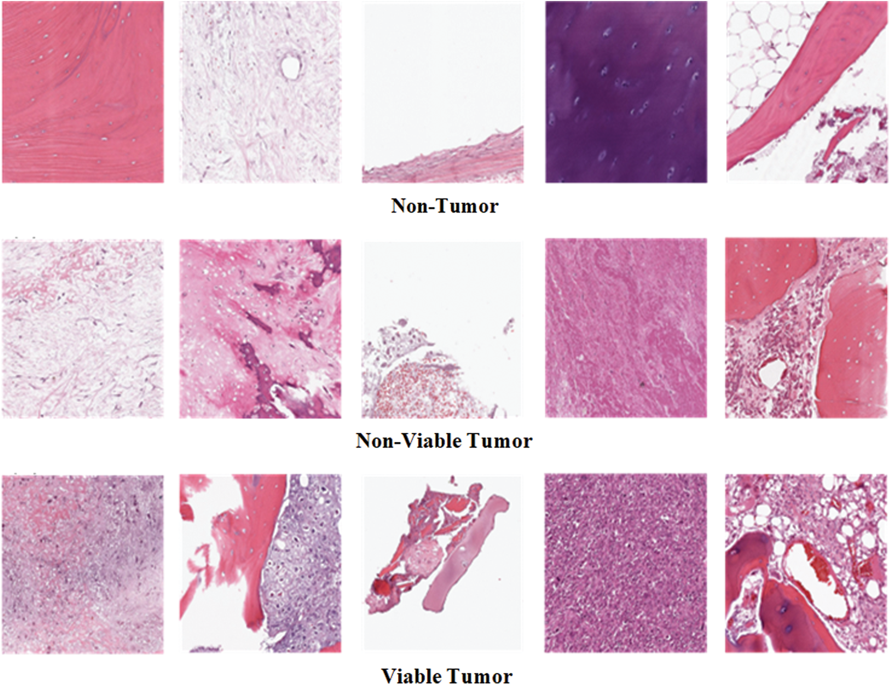
Figure 1: Example images of three classes of osteosarcoma histology image dataset
Osteosarcoma Histology Image Dataset has been used in this research. The dataset can be downloaded from the website of Cancer Imaging Archive (TCIA) [26]. The dataset was collected from the four patients between 1995 and 2015 by a clinical scientist team at the University of Texas Southwestern Medical Center at Children’s Medical Center, Dallas. The dataset is publically available on the TCIA website for research purposes. The dataset comprises 1144 Hematoxylin and Eosin stained histology images of Osteosarcoma having an image size of 1024 × 1024 pixels. The dataset consists of three classes of histology images: 1. Non-Tumor (NT), 2. Non-Viable Tumor (NVT), 3. Viable Tumor (VT). The majority class of the dataset is Non-Tumor that contains 536 images of normal tissues of bone, blood vessels, and cartilage. Non-Viable Tumor and Viable Tumor are minority classes of a dataset with 263 and 345 images, respectively. NVT class contains images of death or the stage of recovery tissues having a relatively light color. VT is a region in histology images where Nuclei are densely accumulated together in dark color. Fig. 1 shows some example images of all three classes. Tab. 1 explains the detail of the imbalanced distribution of histology images within the dataset.

In this work, we present a CNN-based automated Osteosarcoma histology image classification mechanism. The proposed mechanism consists of four modules, i.e., Dataset Collection Module, Imbalanced Classes Balancing Module, Classification of Histology Images Module, and CNN Models Evaluation Module. The details of the proposed mechanism are illustrated in Fig. 2.
In Dataset Collection Module, the histology images of the Osteosarcoma dataset are arranged into three classes of NT, NVT, and VT. The second module, i.e., the Imbalanced Classes Balancing Module, is divided into four steps. In the first step, after collecting histology images dataset with imbalanced classes, the dataset is precisely observed, and the number of images of each class is recorded; the dataset is divided into two groups: majority class and minority classes. In the second step, the Oversampling technique has been applied to minority classes to equalize the number of images in all classes. The required number of histology images for each minority class has been formed through photo creator and editor software utilizing different functions for class balancing. A histology images dataset is designed with balanced classes by adding artificial images into minority classes in the third step. Finally, the balanced dataset is divided randomly into training and testing with an 80% and 20% ratio.
In the third module, i.e., Classification of Histology Images Module, imbalanced datasets of Osteosarcoma are used to train and test the non-regularized and regularized CNN models. In the non-regularized CNN model, the images are directly processed without applying any image pre-processing techniques. In contrast, in regularized CNN, data augmentation is first applied as an image pre-processing step by utilizing Keras Data Generator for increasing variety in training and testing datasets. At the end of the module, images are classified into one of three classes. In the last module, after the execution of the models, accuracy and loss matrices are recorded, and then the plots are drawn for all four cases, i.e., non-regularized CNN for the imbalanced dataset, non-regularized CNN for a balanced dataset, regularized CNN for an imbalanced dataset and regularized CNN for a balanced dataset. Finally, a comparison is performed for the best and the worst-case using the histology images dataset.
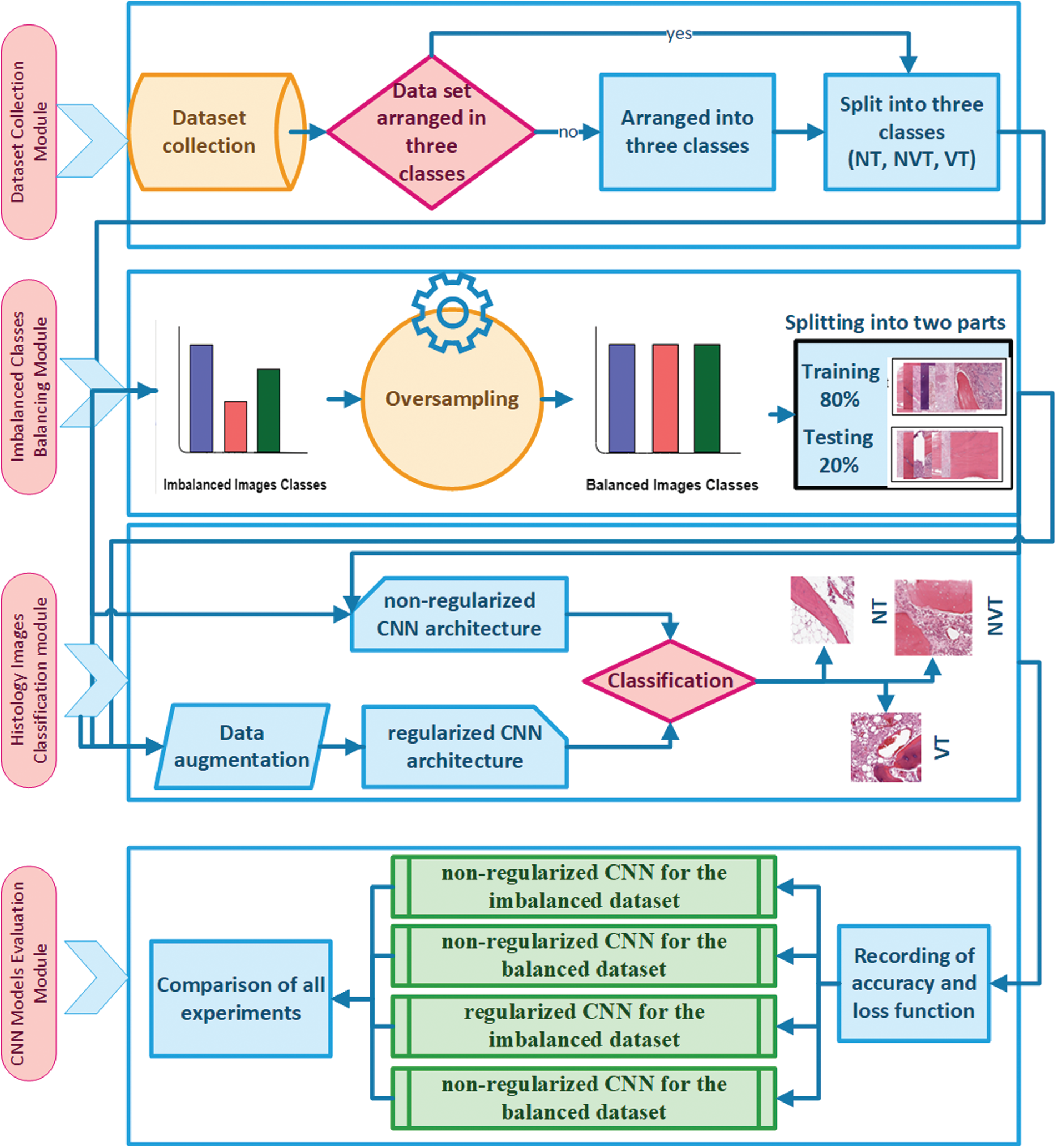
Figure 2: Proposed model with four modules: dataset composing module, imbalanced classes balancing module, classification of histology images module, and CNN models evaluation module
4.1 Oversampling for Balancing ICD
Osteosarcoma images dataset contain imbalanced class distribution. In ICD, CNN models are mostly biased towards the majority class, and images of minority classes usually do not predict accurately. For accurate classification and prediction of minority class images, equaling the number of images in all classes can be immensely beneficial. There exist two main ways, i.e., data level and class level, for balancing the data samples in classes. Data levels are pre-processed techniques directly applied to unequal data samples of classes to balance the number of data samples of the dataset. At the data level, two popular and effective techniques are oversampling and under-sampling. In oversampling, data samples are added in minority classes to meet the majority class level. In under-sampling, data samples are eliminated from majority classes to make all classes equal. The algorithmic level techniques are mostly employed to design a new algorithm or improve existing algorithms' performance to tackle the dataset's imbalanced data distribution. Cost-sensitive methods and one cost learning are famous Algorithmic level solutions. In cost-sensitive methods, higher misclassification cost is assigned to the minority examples. One-class learning techniques address the imbalanced class problem by transforming the training mechanism and attain better accuracy for the minority classes. Instead of differentiating examples of one class from the others, these techniques learn a model by utilizing mainly or only a single class example.
For accurate classification of small histology images dataset, the Oversampling technique has been utilized for balancing all classes. If the majority class contains the number of images represent by MajCl and minority classes contain,
In Oversampling, new synthetic images are added in minority classes to equalize samples in all classes. In minority class 1
In the Osteosarcoma histology images dataset, the difference of images between NT and NVT is 101 and between NT and VT is 156. So, 101 NVT and 156 VT images are needed to be synthesized for balancing the classes. Due to technological advancement, several photo editors and 3D image Creator software are available with various features and functions that can be used to generate quite realistic images. In this work, Photo Editor Software has been utilized for generating the required number of histology images from the original images for balancing the data in all classes. First, the original images are randomly selected from the minority classes. The rotating function is applied to the selected image, and the image is rotated at 180 degrees. After rotation, a contrast feature is utilized, and then the 3D effect is applied to the image to capture an image with different perspectives. The resulting images are saved with a size of 1,024 × 1,024 pixels. Finally, the newly generated images are mixed with the original NVT and VT classes to form balanced class datasets. Some synthesize images from NVT and VT are shown in Fig. 3. The bar chart representation of actual and balanced classes is shown in Fig. 4.
4.2 Convolutional Neural Network Architectures
In this work, two CNN models, i.e., non-regularized CNN and regularized CNN, have been designed to accurately classify histology images, particularly when the dataset is small. The goal is to investigate the effects of CNN models with the absence and presence of regularization techniques when facing the challenge of overfitting during the classification of histology images of a small dataset. Both CNN models share similarities in terms of architecture; the differences exist on a technical basis as regularized CNN model is combined with three regularization layers. Both CNN model consists of Convolutional section and Dense Section. The convolutional section comprises four convolutional layers and pooling layers, while the Dense Section comprises two dense layers. Both sections are concatenated through flatten layer. The architectural design and functionality are explained as follows.
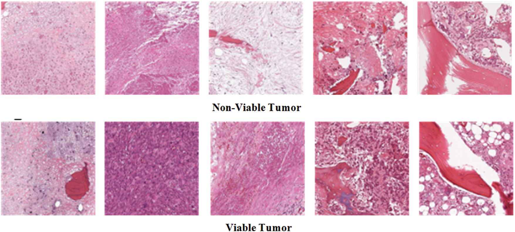
Figure 3: Example osteosarcoma histology synthesized images
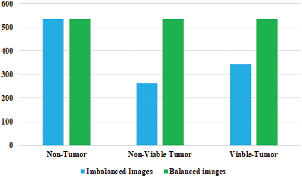
Figure 4: Detail of osteosarcoma image dataset with balanced distribution
There are two main components in convolution layers, i.e., size of filter and number of filters. Filters are utilized for extracting features by convolving a filter (F) of size f × f to an input image (I) of the size I × I. In the designed approach, all four convolution layers filter size is fixed to 3 × 3. The number of filters defined output is called features map. All four convolutional layers define various feature maps; here, the number of feature maps are 32, 64, 128, and 256 for successive convolution layers shown in Fig. 5. The distance between two successive kernel positions is called stride (s); each convolution layer stride is set to 1. To avoid shrinking the feature map and producing the same size as the input matrix, zero paddings is combined across the input matrix's borders. Various feature maps are calculated by repeating the process and by utilizing filters of different sizes and values. The result is summed up to obtain a single output value in the corresponding position of the output tensor called Feature Map of size (w × h). The convolution operation for one pixel for the feature map (FM) is mathematically calculated [27,28].
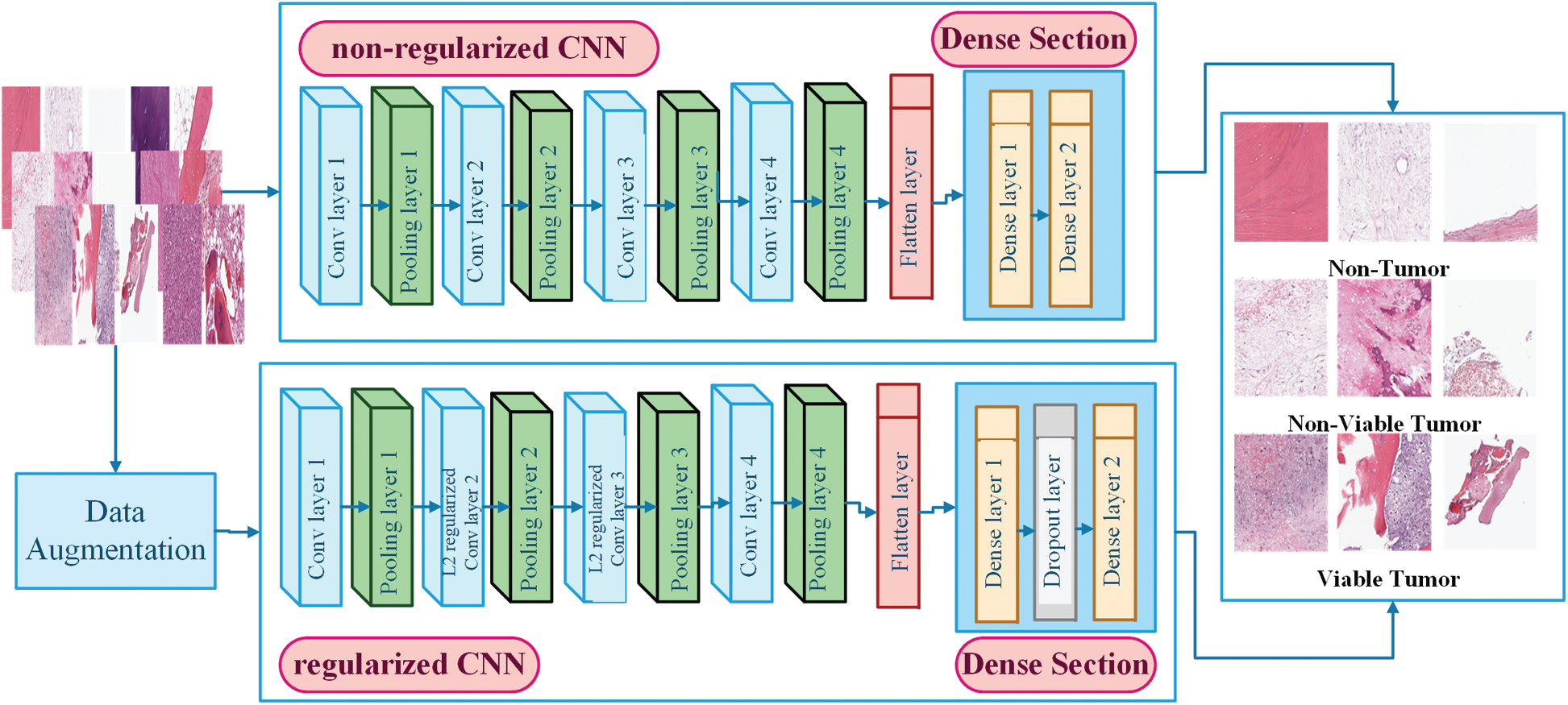
Figure 5: Architecture of non-regularized and regularized CNN models
Mathematically output size of FM with padding P is calculated as [29].
In Eq. (4)
Both CNN models have four pooling layers with 2 × 2 patch sizes; it has been applied for the down-sampling of feature maps. In the designed approach, max pooling is utilized for extracting the largest value in each patch from the input feature maps [31], and all the other values are discarded. The function results in down-sampled maps that highlight the most prominent features in the image patch. The max-pooling operation is estimated as [31];
In Eq. (6),

Flatten layer then converts (16, 16) output shape to a single 32,768 nodes passed to fully connected layers. Two dense layers have been utilized in the design of the CNN model. The first dense layer contains 512 and the second dense layer contains three nodes. ReLU has been defined as an activation function in the first dense layer, while in the second, the softmax is applied as an activation function for categorical classification. Mathematically the softmax is represented as [32];
In Eq. (7)
The first dense layer connects each flattened node (32,768 nodes) from flatter layers to 512 nodes and calculates a high number of 16,777,728 parameters as it creates maximum parameters. The second dense layer classifies images by utilizing the categorical function ‘softmax’ into one of three classes and calculates 1559 parameters with 512 nodes of the previous layer and three targeted nodes.
Regularized CNN consists of two convolution layers, two L2 regularized convolution layers, four pooling layers, two dense layers, and one dropout layer. The general architecture of regularized CNN model is shown in Fig. 5. This model is designed to combat the overfitting problem. We performed three regularization techniques and integrated them with a non-regularized CNN model to make it regularized. The utilized regularization techniques are data augmentation, L2 Regularization, and dropout Layer. In data augmentation, images are artificially inflated the original training dataset by using label preserving transformations to add more invariant examples.
In this work, Keras Data Generator has been applied for data augmentation. L2 Regularization is a common way to mitigate overfitting by putting constraints on a network's complexity by forcing its weights to take only small values, making the distribution of weight values more regular. L2 Regularization technique forces the weight to reduce but never makes them zero. In Regularized CNN model, L2 Regularization has been used in the second and third convolution layers to reduce overfitting and complexity of the model and produce an accurate histology image classification.
5 Experimental Results and Discussion
This research work has been implemented using the Python programming language with Google Colab. The Neural Network library ‘Keras’ is utilized to design, compile, and evaluate the proposed CNN models. The models have experimented with different learning rate values, batch size, epochs, and steps per epoch for achieving the maximum classification accuracy. Finally, the models are evaluated with fixing epoch to 45, batch size to 100, learning rate to 0.001, and steps per epoch to 20. ‘Adam’ and categorical cross-entropy are used as Optimizer and Loss function, respectively. Regularized CNN model, data augmentation technique, and non-regularized CNN model have experimented with for classification of histology images of Imbalanced and Balanced dataset. After the execution of models, accuracy and loss matrices are recorded for each experiment, and then the comparison is performed to find the best and worst cases. The detail of all experiments is shown in Tab. 3. The detailed description of experiments is described in sub-sections.

5.1 Classification of Small Imbalanced Histology Dataset Using Non-Regularized CNN Model
The first experiment is performed for a small Imbalanced complex Osteosarcoma dataset. The imbalanced dataset is trained and tested using a Non-Regularized CNN. In this experiment, huge overfitting was observed with a 20% and 11.52% difference of training and testing accuracy for the Osteosarcoma dataset. The training accuracy is 98%, and the testing accuracy is 78% achieved for the Osteosarcoma dataset. The accuracy and loss plots of the first experiment are shown in Fig. 6.
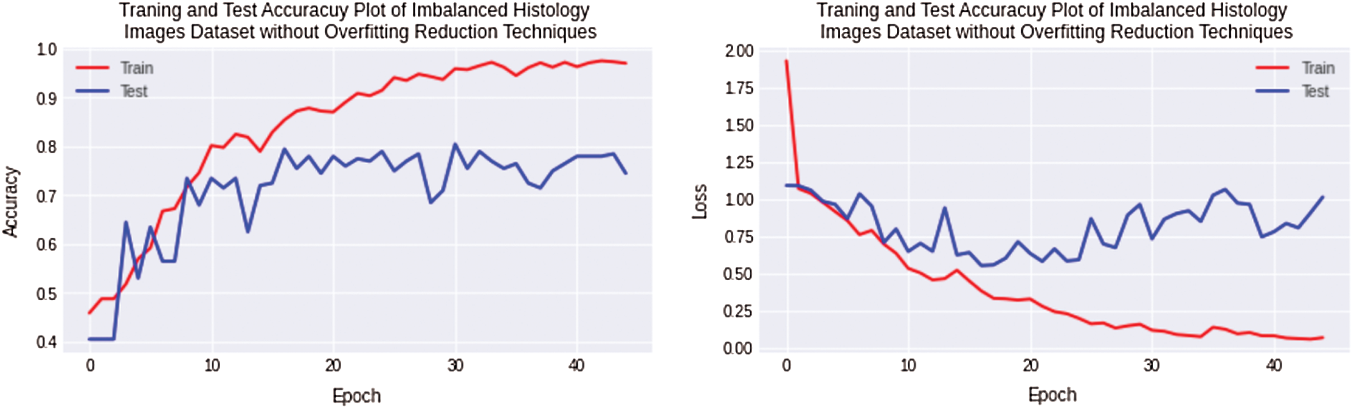
Figure 6: Training and testing accuracy plot on the left side and loss error plot on the right side show high overfitting for imbalanced Osteosarcoma images dataset by using non-regularized CNN model
5.2 Classification of Small Balanced Histology Dataset Using Non-Regularized CNN Model
The second experiment is performed to reduce overfitting and improve testing accuracy. The balanced datasets of Osteosarcoma are created by adding artificial histology images synthesized in photo editor software for equalizing images. In this experiment, overfitting is still observed 15% for the Osteosarcoma dataset, but as the balanced dataset is used, 5% of the overfitting value has been reduced. Non-Regularized CNN along with Osteosarcoma balanced dataset achieved 96% and 81% training and testing accuracy. The accuracy and loss plots of the second experiment are shown in Fig. 7.
5.3 Classification of Small Imbalanced Histology Dataset Using Regularized CNN Model
In the first and second experiments, overfitting is observed for the small histology images dataset classification with non-regularized CNN. The design of 11 layers CNN model is modified by adding regularization techniques. In this experiment, classification was performed for images of Imbalanced histology datasets using regularized CNN and data augmentation technique. Thus, experiments show that overfitting is decreased and reached 9% for the complex histology dataset, while the accuracy and loss plot is shown in Fig. 8.
5.4 Classification of Small Balanced Histology Dataset Using Regularized CNN Model
Finally, the experimentation has been performed for a balanced histology images dataset using regularized CNN model. The regularized CNN model achieves the best results for a balanced dataset, and the overfitting value decreased to 1% for the complex Osteosarcoma dataset. Testing accuracy achieved high numbers up to 86%, better than all experiments. The accuracy and loss plot is shown in Fig. 9. If the results are compared with previous ones, it can be observed that overfitting has been significantly reduced.
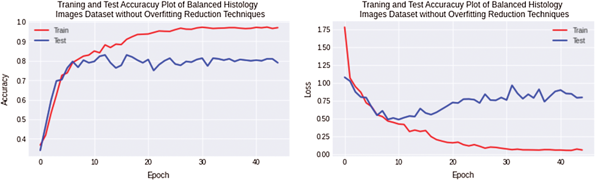
Figure 7: Training and testing accuracy plot on the left side and loss error plot on the right side show high overfitting for balanced osteosarcoma images dataset by using non-regularized CNN model
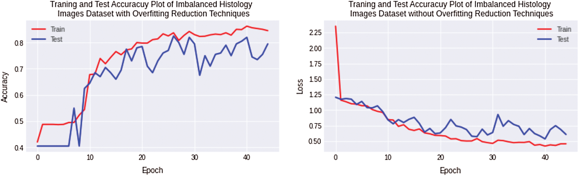
Figure 8: Training and testing accuracy plot on left side and loss error plot on the right side show overfitting reduction with a combination of imbalanced osteosarcoma image dataset with regularized CNN model
We compare the results of the above four discussed scenarios; it can be concluded that the non-regularized CNN model does not achieve good/suitable for small histology images dataset because simple CNN fails to obtain generalization and suffers from overfitting problems. Similarly, an imbalanced dataset with unequal classes fails to achieve a better result. Fig. 10 shows that the comparison results of all four complex Osteosarcoma's testing accuracy; it can be seen that the regularized CNN model for a balanced dataset achieved high accuracy. Same as in Fig. 11, comparison results of testing loss error for all four experiments of Osteosarcoma Dataset has been plotted; the Figure shows that regularized CNN classifies histology images with less error rate for balanced dataset.
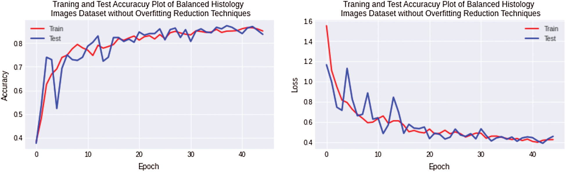
Figure 9: Training and testing accuracy plot on the left side and loss error plot on the right side shows the best result. With balanced osteosarcoma images and regularized CNN model, overfitting is almost negligible
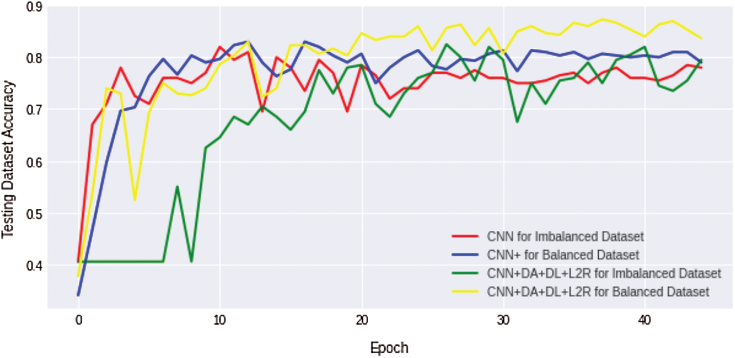
Figure 10: Comparison results of testing accuracy for all four osteosarcoma dataset experiments show that regularized CNN gains high testing accuracy for histology image classification with a balanced dataset
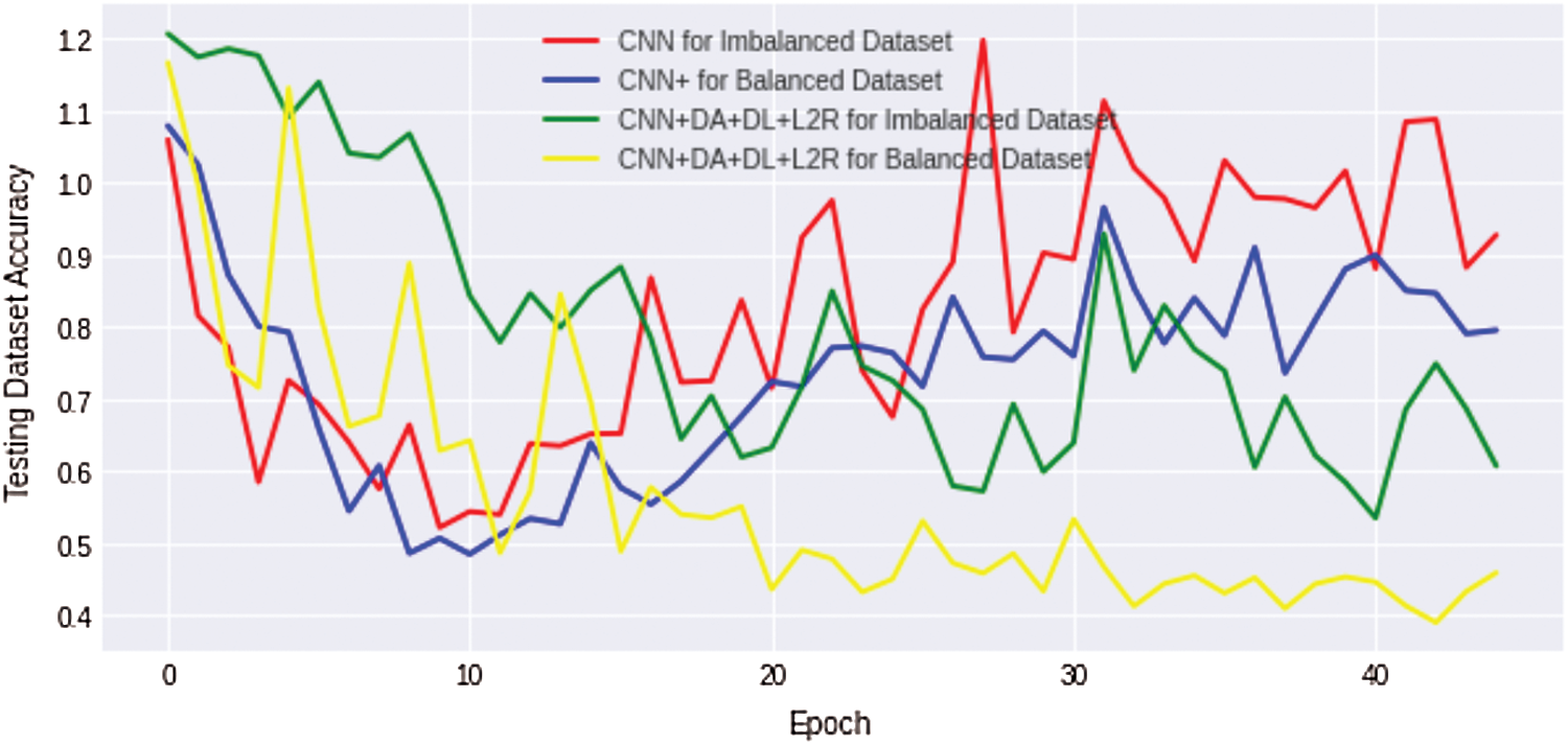
Figure 11: Comparison results of testing loss error for all four osteosarcoma dataset experiments show that regularized CNN classifies histology images with less error rate for a balanced dataset
We also show the comparison results of overfitting for all four experiments in Fig. 12. It can be seen that the overfitting results of a non-regularized CNN model with an imbalanced dataset are high. In contrast, the value of overfitting is minimum with a balanced dataset. The regularized CNN model with an imbalanced dataset shows the lowest overfitting value nearly equals 1%. In Fig. 12 IDS, an Imbalanced Dataset, while BDS indicates Balanced Dataset, NRCNN represents non-regularized CNN and RCNN shows regularized CNN model.
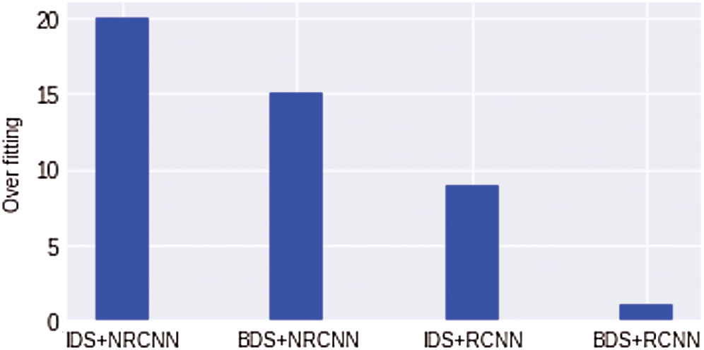
Figure 12: Comparison results for overfitting reduction in all four experiments
In this research work, a compact CNN model for the classification of small imbalanced and balanced Osteosarcoma histology images dataset is proposed. As classification and prediction of a small dataset with CNN architecture are difficult, particularly in microscopy images where similarity within classes strongly exists, it is extremely challenging. Therefore, in this work, firstly, we performed balancing of histology images dataset with oversampling technique. Then two CNN models named non-regularized and regularized are designed. The regularized model is integrated with CNN's basic architecture to reduce overfitting. The results demonstrate that oversampling effectively addresses the class imbalanced problem during training—furthermore, comparison of non-regularized and regularized CNN architecture are performed with imbalanced and balanced histopathology image datasets. The non-regularized CNN model achieves 98% & 78% and 96% & 81% training and testing accuracy with an Imbalanced and balanced histology image dataset. While the regularized CNN model achieved 84% & 75% and 87% & 86% training and testing accuracy with Imbalanced and balanced histology image dataset, respectively. The overfitting values have been reduced from 20% to 1%.
Funding Statement: This research was funded by the Deanship of Scientific Research at Princess Nourah bint Abdulrahman University through the Fast-track Research Funding Program.
Conflicts of Interest: The authors declare that they have no conflicts of interest to report regarding the present study.
1. M. Adeel, M. Asif, M. N. Faisal, M. H. Chaudary, M. S. Malik et al., “Comparative study of adjuvant chemotherapeutic efficacy of docetaxel plus cyclophosphamide and doxorubicin plus cyclophosphamide in female breast cancer,” Cancer Management and Research, vol. 11, pp. 727, 2019. [Google Scholar]
2. M. Galar, A. Fernandez, E. Barrenechea, H. Bustince and F. Herrera, “A review on ensembles for the class imbalance problem: Bagging, boosting, and hybrid-based approaches,” IEEE Transactions on Systems, Man, and Cybernetics, Part C (Applications and Reviews), vol. 42, no. 4, pp. 463–484, 2011. [Google Scholar]
3. M. Alghamdi, M. A. Mallah, S. Keteyian, C. Brawner, J. Ehrman et al., “Predicting diabetes mellitus using SMOTE and ensemble machine learning approach: The henry ford exercise testing (FIT) project,” PLoS One, vol. 12, no. 7, pp. e0179805, 2017. [Google Scholar]
4. M. Ahmad, A. M. Khan, M. Mazzara, S. Distefano, M. Ali et al., “A fast and compact 3-D CNN for hyperspectral image classification,” IEEE Geoscience and Remote Sensing Letters, pp. 1–5, 2021. [Google Scholar]
5. R. Abdulhammed, M. Faezipour, A. Abuzneid and A. AbuMallouh, “Deep and machine learning approaches for anomaly-based intrusion detection of imbalanced network traffic,” IEEE Sensors Letters, vol. 3, no. 1, pp. 1–4, 2018. [Google Scholar]
6. A. Aditsania and A. L. Saonard, “Handling imbalanced data in churn prediction using ADASYN and backpropagation algorithm,” in Proc. of 3rd Int. Conf. on Science in Information Technology, Yogyakarta, Indonesia, pp. 533–536, 2017. [Google Scholar]
7. S. Kim, H. Kim and Y. Namkoong, “Ordinal classification of imbalanced data with application in emergency and disaster information services,” IEEE Intelligent Systems, vol. 31, no. 5, pp. 50–56, 2016. [Google Scholar]
8. L. M. Raposo, M. B. Arruda, R. M. de Brindeiro and F. F. Nobre, “Lopinavir resistance classification with imbalanced data using probabilistic neural networks,” Journal of Medical Systems, vol. 40, no. 3, pp. 69, 2016. [Google Scholar]
9. U. Fiore, A. D. Santis, F. Perla, P. Zanetti and F. Palmieri, “Using generative adversarial networks for improving classification effectiveness in credit card fraud detection,” Information Sciences, vol. 479, pp. 448–455, 2019. [Google Scholar]
10. M. Galar, A. Fernandez, E. Barrenechea, H. Bustince and F. Herrera, “A review on ensembles for the class imbalance problem: Bagging-, boosting-, and hybrid-based approaches,” IEEE Transactions on Systems, Man, and Cybernetics, Part C (Applications and Reviews), vol. 42, no. 4, pp. 463–484, 2011. [Google Scholar]
11. L. Abdi and S. Hashemi, “To combat multi-class imbalanced problems by means of over-sampling technique,” IEEE Transactions on Knowledge and Data Engineering, vol. 28, no. 1, pp. 238–251, 2015. [Google Scholar]
12. V. López, A. Fernández, J. G. Moreno-Torres and F. Herrera, “Analysis of pre-processing vs. cost-sensitive learning for imbalanced classification,” Expert Systems with Applications, vol. 39, no. 7, pp. 6585–6608, 2012. [Google Scholar]
13. https://wiki.cancerimagingarchive.net/pages/viewpage.action?pageId=52756935 [Last accessed on 23 February 2020]. [Google Scholar]
14. J. Ker, Y. Bai, H. Y. Lee, J. Rao and L. Wang, “Automated brain histology classification using machine learning,” Journal of Clinical Neuroscience, vol. 66, pp. 239–245, 2019. [Google Scholar]
15. A. Rehman, M. A. Khan, T. Saba, Z. Mehmood, U. Tariq et al., “Microscopic brain tumor detection and classification using 3D CNN and feature selection architecture,” Microscopy Research and Technique, vol. 84, pp. 133–149, 2020. [Google Scholar]
16. H. B. Arunachalam, R. Mishra, O. Daescu, K. Cederberg, D. Rakheja et al., “Viable and necrotic tumor assessment from whole slide images of osteosarcoma using machine-learning and deep-learning models,” PloS One, vol. 14, no. 4, pp. e0210706, 2019. [Google Scholar]
17. R. Mishra, O. Daescu, P. Leavey, D. Rakheja and A. Sengupta, “Convolutional neural network for histopathological analysis of osteosarcoma,” Journal of Computational Biology, vol. 25, no. 3, pp. 313–325, 2018. [Google Scholar]
18. Y. Fu, P. Xue, H. Ji, W. Cui and E. Dong, “Deep model with Siamese network for viable and necrotic tumor regions assessment in osteosarcoma,” Medical Physics, vol. 47, no. 10, pp. 4895–4905, 2020. [Google Scholar]
19. D. M. Anisuzzaman, H. Barzekar, L. Tong, J. Luo and Z. Yu, “A deep learning study on osteosarcoma detection from histological images,” Computer Vision and Pattern Recognition, pp. 1–10, 2020. [Google Scholar]
20. N. V. Chawla, K. W. Bowyer, L. O. Hall and W. P. Kegelmeyer, “SMOTE: Synthetic minority over-sampling technique,” Journal of Artificial Intelligence Research, vol. 16, pp. 321–357, 2002. [Google Scholar]
21. M. D’Acunto, M. Massimo and M. Davide, “From human mesenchymal stromal cells to osteosarcoma cells classification by deep learning,” Journal of Intelligent & Fuzzy Systems, vol. 37, no. 6, pp. 7199–7206, 2019. [Google Scholar]
22. M. D’Acunto, M. Massimo and M. Davide, “Deep learning approach to human osteosarcoma cell detection and classification,” in Int. Conf. on Multimedia and Network Information System, Cham, Springer, pp. 353–361, 2018. [Google Scholar]
23. R. Mishra, D. Ovidiu, L. Patrick, R. Dinesh and S. Anita, “Histopathological diagnosis for viable and non-viable tumor prediction for osteosarcoma using convolutional neural network,” in Int. Sym. on Bioinformatics Research and Applications, Cham, Springer, pp. 12–23, 2017. [Google Scholar]
24. H. B. Arunachalam, R. Mishra, A. Bogdan, D. Ovidiu, M. Maria et al., “Computer-aided image segmentation and classification for viable and non-viable tumor identification in osteosarcoma,” in Pacific Symp. on Biocomputing 2017, Kohala Coast, Hawaii, USA, pp. 195–206, 2017. [Google Scholar]
25. P. Leavey, A. Sengupta, D. Rakheja, O. Daescu, H. B. Arunachalam et al., “Osteosarcoma data from ut southwestern/UT Dallas for viable and necrotic tumor assessment [data set],” Cancer Imag. Arch., Fayetteville, AR, USA, Tech. Rep, 2019. [Google Scholar]
26. K. Clark, B. Vendt, K. Smith, J. Freymann, J. Kirby et al., “The cancer imaging archive (TCIAMaintaining and operating a public information repository,” Journal of Digital Imaging, vol. 26, no. 6, pp. 1045–1057, 2013. [Google Scholar]
27. K. F. Alam, B. Ateeq, M. Asif, W. Ahmad, M. Nawaz et al., “Computer-aided diagnosis for burnt skin images using deep convolutional neural network,” Multimedia Tools and Applications, vol. 79, pp. 34545–34568, 2020. [Google Scholar]
28. D. Stutz, “Seminar report: Understanding convolutional neural networks,” Fakultät für Mathematik, Informatik und Naturwissenschaften Lehr-und Forschungsgebiet Informatik VIII, Seminar Report, 1–23, 2014. [Google Scholar]
29. S. Albawi, T. A. Mohammed and S. Al-Zawi, “Understanding of a convolutional neural network,” in Proc. of IEEE Int. Conf. on Engineering and Technology, Antalya, Turkey, Akdeniz University, pp. 1–6, 2017. [Google Scholar]
30. R. H. Hahnloser, R. Sarpeshkar, M. A. Mahowald, R. J. Douglas and H. S. Seung, “Digital selection and analogue amplification coexist in a cortex-inspired silicon circuit,” Nature, vol. 405, no. 6789, pp. 947–951, 2000. [Google Scholar]
31. O. Abdel-Hamid, A. R. Mohamed, H. Jiang and G. Penn, “Applying convolutional neural networks concepts to hybrid NN-HMM model for speech recognition,” in Proc. of IEEE Int. Conf. on Acoustics, Speech and Signal Processing, Kyoto, Japan, pp. 4277–4280, 2012. [Google Scholar]
32. Y. Wang, Y. Li, Y. Song and X. Rong, “The influence of the activation function in a convolution neural network model of facial expression recognition,” Applied Sciences, vol. 10, no. 5, pp. 1897, 2020. [Google Scholar]
 | This work is licensed under a Creative Commons Attribution 4.0 International License, which permits unrestricted use, distribution, and reproduction in any medium, provided the original work is properly cited. |