DOI:10.32604/cmc.2021.018546
| Computers, Materials & Continua DOI:10.32604/cmc.2021.018546 | |
| Article |
Cloud Data Center Selection Using a Modified Differential Evolution
1National Advanced IPv6 Center (NAv6), Universiti Sains Malaysia, 11800 USM, Penang, Malaysia
2Computer Science Department, PY Collage, Northern Border University (NBU), 9280 NBU, Ar’ar, Kingdom of Saudi Arabia
*Corresponding Author: Mohammed Anbar. Email: Anbar@usm.my
Received: 12 March 2021; Accepted: 13 April 2021
Abstract: The interest in selecting an appropriate cloud data center is exponentially increasing due to the popularity and continuous growth of the cloud computing sector. Cloud data center selection challenges are compounded by ever-increasing users’ requests and the number of data centers required to execute these requests. Cloud service broker policy defines cloud data center’s selection, which is a case of an NP-hard problem that needs a precise solution for an efficient and superior solution. Differential evolution algorithm is a metaheuristic algorithm characterized by its speed and robustness, and it is well suited for selecting an appropriate cloud data center. This paper presents a modified differential evolution algorithm-based cloud service broker policy for the most appropriate data center selection in the cloud computing environment. The differential evolution algorithm is modified using the proposed new mutation technique ensuring enhanced performance and providing an appropriate selection of data centers. The proposed policy’s superiority in selecting the most suitable data center is evaluated using the CloudAnalyst simulator. The results are compared with the state-of-arts cloud service broker policies.
Keywords: Cloud computing; data center; data center selection; cloud service broker; differential evolution; user request
A data center (DC) is a set of essential shared resources, including but not limited to servers, network devices, power systems, data storage, and cooling systems [1]. A traditional DC is a physical site where all servers are located, but a cloud DC is a set of shared computing resources with higher Quality-of-Service (QoS) at a lower total cost of ownership [2]. However, the main difference between traditional DC and cloud DC is virtualization that provides enormous scalability, virtualized computing resources, and on-demand utility computing.
DC virtualization is a precious opportunity for IT. It saves the cost to a remarkable extent by efficiently sharing the available resources, such as servers, storage, and network capabilities, translating into lower purchasing and operating costs. The DC virtualization provides compatibility with more applications and services and fast implementation at a higher QoS level. Cloud Computing (CC) technology advancement utilizes DC virtualization as a springboard to access cloud services provided by third-party Cloud Service Providers (CSPs) to build private CC platforms with many of the same economies and efficiencies as by third-party CSPs.
Nowadays, cloud DC demand is increasing due to the importance of speed in IT service delivery. Cloud DC speeds up service delivery by providing processing and storage capabilities and networking close to the users from different locations worldwide. Besides, increased demand for business agility and cost-saving with a high QoS level has led to the rapid growth of cloud DCs over traditional DCs. Also, the CC services have increased rapidly in number and scale across different application areas. Fig. 1 below is from Cisco’s report in 2018, showing the total amount of cloud DC traffic in 2017 reaching 7.7 Zettabyte and 9.8 Zettabyte in 2018. It is projected to reach 11.9 Zettabyte and 14.1 in 2019 and 2020, respectively [3].
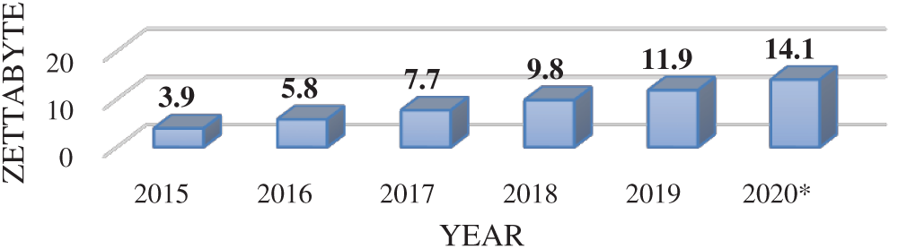
Figure 1: Total annual data center traffic from 2015–2020 [3]
With an increased volume of cloud services generated and data volume stored across geo-distributed DCs, the question of how to route users’ requests in a manner that ensures efficient resource utilization and a high level of QoS has become an emerging topic. Also, the target DC location has a direct influence on the CC environment’s QoS level. An appropriately selected cloud DC will enhance a large-scale CC environment’s overall performance for user requests’ execution by providing efficient resource usage, reduces processing and response time, provides scalability, and averts deadlock [4]. Also, the increased demand for CC’s services makes cloud users more aware of higher-level QoS. This awareness raises a new challenge on efficient and optimal cloud DC selection to cater to different user’s needs from a large set of cloud DCs distributed among different regions worldwide.
1.1 Problem Formulation of Cloud Data Center Selection
cloud DCs communicate with each other in an ad-hoc manner within the CC environment [5 –7] to execute users’ requests. Therefore, similar to selecting a physical DC, the cloud DC must be chosen appropriately for efficient user requests’ execution with minimum computational time and the lowest cost, which remains challenging in the CC field. The following example clarifies the main problem of cloud DC selection.
Assume there are N user requests UR= {UR1, UR2,
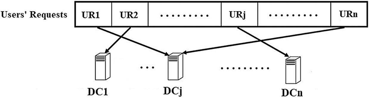
Figure 2: Cloud DC selection problem: routing n users’ requests to n DCs
An improper cloud DC selection overloads the cloud DC. It degrades the CC environment’s performance, especially when there is an expanding number of users’ requests, resulting in the perceived QoS and user satisfaction deteriorating. Consequently, the cloud DCs will drop and refuse any new user request because they are overloaded [8,9].
Several prior works attempted to address the cloud DC selection problem by proposing CSB policies in the CC environment. However, the primary challenge of achieving the maximum performance with the minimum cost remains [10,11]. Several related works such as [12,13] considered the cloud’s DC selection and resource allocation an NP-hard problem; therefore, this paper pertains to adopt a metaheuristic based CSB policy to overcome the improper cloud DC selection due to the following reasons:
• Processing time and response time and/or a high total cost still require more enhancements during the execution of user requests.
• To ensure adaptive user request execution, the DC selection assumptions should consider incoming user requests’ size, which will avoid inaccurate estimation of the processing time.
• The efficient selection of the most appropriate DC requires consideration of more important DCs parameters.
• There is a lack of multi-objective optimization usage in terms of cloud users’ QoS needs; few CSB policies only use a single (simple or complex) optimization objective.
This paper contributes to the literature on service provisioning and CSB policies by highlighting the significance of using multi-objective optimization in selecting the cloud DC to execute users’ requests. This paper’s unique contribution is that it incorporates more than one QoS (i.e., users’ interest) simultaneously when executing users’ requests.
Improper selection of cloud DCs is time and resource-consuming because the same cloud DC executes many users’ requests while others remain idle. Improper cloud DC selection negatively impacts the QoS, especially when user requests executions require a high QoS level. As a result, the DC will drop any new users’ requests because the DCs are busy responding to users’ requests [8,9]. To address the problem mentioned above, any new users’ requests must be routed to the most appropriate cloud DC, which is the responsibility of the CSB to ensure high performance of the CC environment and to execute these users’ requests efficiently with a high level of QoS.
Indeed, proposing an efficient CSB policy grabs the researchers’ attention to address the issues related to selecting the proper cloud DC in the CC environment. The existing CSB policies might be commonly categorized based on users’ QoS needs into (i) CSB policy based on enhancing response and processing time, (ii) CSB policy based on enhancing DC availability, and (iii) CSB policy based on enhancing the total cost.
The CSB policy based on enhancing processing and response time, such as [4,5], suffers from several setbacks because most of them ignore the DC availability and efficiency parameters. Also, the DC selection assumptions do not take the size of the subsequent user request into consideration (i.e., the DC selection assumption is built based on the previously executed users’ requests); thus, inaccurate DC selection has occurred. Therefore, there are still gaps in these considerations because the CC environment’s overall performance might be impacted negatively.
Meanwhile, the proposed CSB based on enhanced availability, such as [6] and [14], increases the cloud DC availability and slightly enhances computation time. Despite its advantages, those policies ignore the dynamic nature of user requests’ size (i.e., different users’ requests may have different sizes). Besides, the DC selection assumption does not take the size of the subsequent users’ requests into consideration, and the total cost is not as reduced as needed.
Moreover, many researchers proposed several CSB policies to decrease the total cost consumed by the cloud DCs to execute users’ requests [15,16], which successfully acheive significant results in reducing the total cost. However, the processing and response time requires more improvements, and the number of executed users’ requests is not always as expected (i.e., throughput is relatively low). Furthermore, these CSB policies are only concentrating on enhancing the performance in terms of the total cost, but also still gaps exist in these CSB policies in terms of ignoring important parameters when selecting DCs, which is one of the considerations in this paper.
Also, all CSB policies in the literature are based on a single (i.e., simple or complex) optimization objective. At the same time, none uses multi-objectives in the cloud DC selection process. Therefore, a multi-objective might enhance DCs selection, as the multi-objective includes more than one parameter (i.e., objective), which will not focus on one parameter. For instance, some users look for services with the lowest cost, while others require high QoS level services, which is acceptable. However, it would not be efficient in the future, especially with an expanding number of users’ requests and connected cloud DCs. Therefore, implementing a multi-objective problem-based cloud DCs selection technique might be highly required. The use of CSB policies based on metaheuristic to provide an efficient cloud DCs selection is also needed, as considered in this paper.
The Differential Evolution (DE) algorithm is arguably one of the most robust stochastic optimization algorithms applied on real-parameter. It is still adapted or modified by researchers for solving optimization problems [17–19]. For instance, a modification on the DE algorithms was proposed in [17] to overcome constrained optimization problems by adaptively adjusting the scale factor and crossover rate based on uniform distribution. Thus, both global and local searches are balanced, which allows efficient exploration of the solution space.
3 Differential Evolution Algorithm
The DE algorithm was developed by Price and Storn in 1997 [20] to solve optimization problems for continuous domains. The DE is considered one of the best optimization algorithms due to its simplicity, easiness, quickness, and robustness [21]. Many different scientific applications use the DE algorithm to obtain the most effective solution without using complicated algorithms or experts’ knowledge [20,21]. The DE uses the mutation phase as a search and selection technique to search for feasible solution regions (i.e., possible solution regions). It is a search mechanism based on the population with vector parameters for every generation. The DE algorithm consists of the following four main phases, namely: (i) initialization, (ii) mutation, (iii) recombination, and (iv) selection. The following sub-sections discuss these phases in detail.
DE is a population-based search algorithm that uses NP variables as the D dimensional parameters population (i.e., vectors) for each search generation. Initially, if there is no information about the problem, the initial population is selected randomly; otherwise, the initial population using DE is usually generated by adding random deviations that are normally distributed to the preliminary solution. The core idea behind the differential evolution is a new technique for generating trial parameter vectors [21]. In our optimization problem, the DCs in each simulation scenario is considered the NP variables. The proposed DCs’ parameters are considered D dimensional vectors (i.e., 4-dimensional vectors: DCAV, DCEff, TotC, ExptPT). The dimensional vector for each generation is computed for each variable that belongs to solution space, as illustrated in the following formula:
where
The mutation phase is the second phase of the DE algorithm. In this phase, a noisy random vector is generated for each generation using Eq. (2) [22]:
where V
The variable resulted from this stage (i.e., Vi, G+1) is called a noisy random vector is used in the next stage to be compared with the target vector based on a crossover rate.
This phase is crucial because it is responsible for increasing the diversity of vectors. In this stage, the noisy random vector resulting from the previous stage (i.e., Vi, G+1) is compared with the target vector (i.e., DC1) to generate a trial vector. Eq. (3) is used to generate a trial vector.
where Y
For instance, assume the value of CR is 0.50, and the rndb(n) values for the four-dimensional parameters are as follows: 0.7, 0.2, 0.3, 0.5 for DCAV, TotC, ExpPT, and DCEff, respectively. Since 0.7 ¿ 0.5 = ¿ yes, the value of the DCAV dimensional parameter associated with the target vector is copied. Besides, 0.2 ¿ 0.5 = ¿no, the value of the TotC dimensional parameter associated with the noisy random vector is copied. While 0.3 ¿ 0.5 = ¿ no, the value of the ExptPT dimensional parameter associated with the noisy random vector is copied. Last, since 0.9 ¿ 0.5 = ¿ yes, the value of the ExptPT dimensional parameter associated with the target vector is copied. However, this phase’s output is a trial vector (Yi, G+1) with dimensional parameter values.
The last phase of the DE is the selection phase. In this phase, a greedy criterion is used to determine whether the trail vector’s fitness function (Y
IF (F (Y
X
else
Retain Xn1, G
This section describes the proposed policy phases, called High-Performance Lowest Cost CSB (HPLCCSB) policy. In a real cloud environment, the proposed CSB policy operates in an online mode since the users’ requests arrive through the Internet. However, for experimental purposes, the proposed CSB policy is evaluated in offline mode since conducting repeatable experiments in large-scale environments such as a real cloud environment is very complex and time-consuming [6] and [24].
Fig. 3 depicts the main phases of this policy. Upon receiving a new user’s request, the fitness function of each DC is computed based on the proposed DC’s parameters. Then the modified DE is adapted to find the most optimal DC among the available DCs (in terms of the value of fitness function). After that, the arriving user’s request is routed to this DC to execute it and return it to its originator (i.e., user base).
4.1 Data Centers’ Parameters Computation
In this phase, four main parameters are computed in order to be contributed to formulating the fitness function (i.e., multi-objective function). These parameters are considered the most important parameters that might characterize the DCs [25,26]. Therefore, considering these parameters during the selection phase could allow optimal DC selection with the best computational capabilities with the lowest cost. As aforementioned, most existing studies focus only on one and only one parameter without considering others. Thus, part of QoS might be improved and others not. Therefore, it is necessary to incorporate these crucial parameters to formulate a multi-objective function that ensures optimal value.
However, the data center availability parameter is one of the most important DC parameters that describes the ratio between throughput and available bandwidth for each cloud DC is computed based on Eq. (4).
where DCAV denotes the DC availability parameter, TH[x,y] denotes cloud DC throughput, obtained from the InternetCharacteristics component in the CloudAnalyst, and BN[Nx, My] denotes bandwidth matrix for cloud DC(y), located in a region(x).
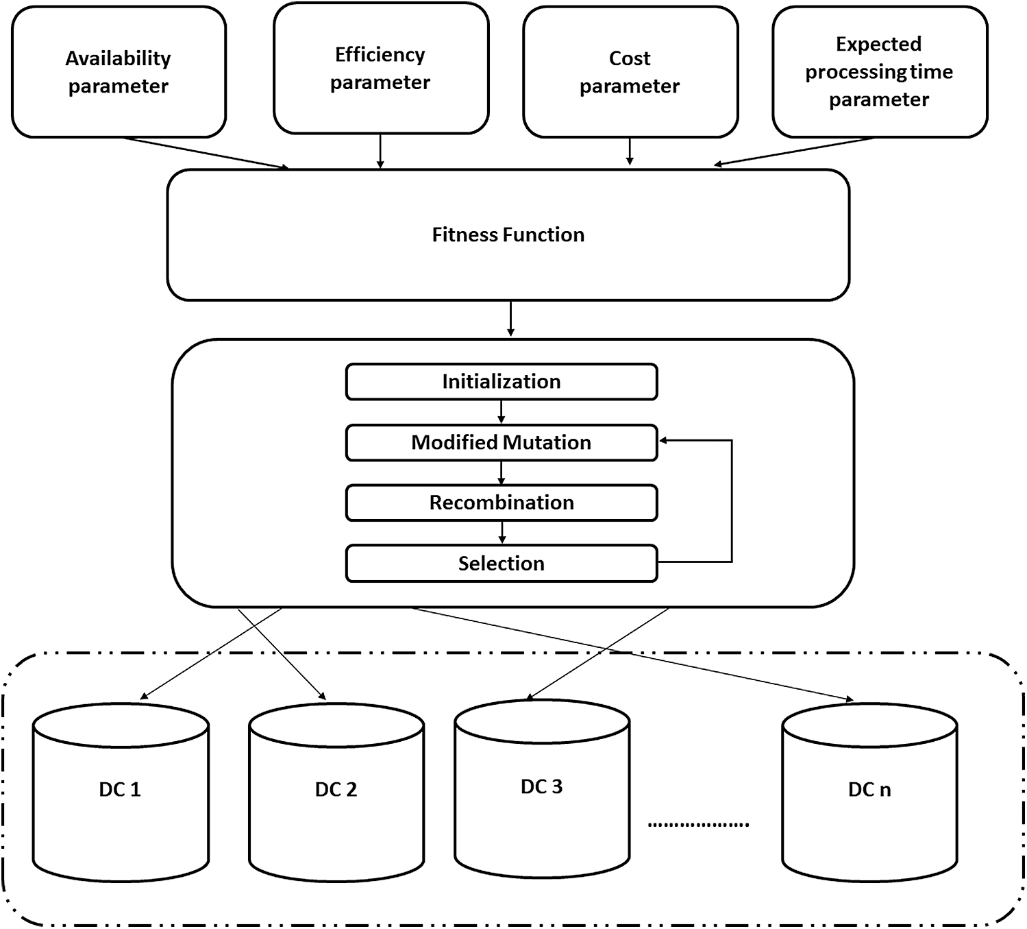
Figure 3: Proposed policy
Each cloud DC’s expected processing time parameter describes the estimated processing time required to execute the incoming users’ requests. This parameter is computed based on Eq. (5).
where ExpPT denotes the expected processing time for the subsequent user request, NxURS denotes the subsequent user request’s size determined from the InternetCloudlet component in the CloudAnalyst simulator, AVGPR denotes the average processing ratio for DC, computed using Eq. (6).
where AEUR denotes the average size of previously executed users’ requests determined from the DatacenterController component in the CloudAnalyst simulator, AVGPT denotes the average processing time for the previously completed users’ requests, which is also obtained from the DatacenterController component by dividing the total processing time on the total number of executed users’ requests by a given cloud DC.
Third, the total cost parameter describes the consumed cost (in US dollars) to execute and deliver the user requests to the user. This parameter is computed based on Eq. (7).
where TotC denotes total cost, DTC denotes data transfer cost, and VMC denotes virtual machine (VM) cost.
Last, the DC efficiency parameter describes how efficient a DC is in executing the users’ requests. This parameter is computed based on Eq. (8).
where DCEff denotes the DC efficiency, ART denotes average response time obtained from the VMLoadBalancer component in the CloudAnalyst simulator, APT denotes average processing time obtained from DatacenterController in the CloudAnalyst simulator. AWT denotes the average waiting time obtained from VMLoadBalancer in the CloudAnalyst simulator. Thr denotes throughput for each DC obtained from the InternetCharacteristics component in the CloudAnalyst simulator. UsT denotes total useful time for each processor obtained from the DatacenterController component in the CloudAnalyst simulator. IdT denotes a total idle time for each processor obtained from the DatacenterController component in the CloudAnalyst simulator. NoVM denotes the number of the virtual machines located in each cloud DC, which is also obtained from the DatacenterController component in the CloudAnalyst simulator.
4.2 Fitness Function Computation
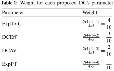
This phase proposes the fitness function derived from the values of the previously proposed parameters (i.e., DCAV, ExpPT, TotC, and DCEff). The proposed fitness function uses the scalarization method based on rank-sum weights [27,28], where all objectives functions are incorporated altogether into the scalar fitness function. Eq. (9) computes the value of DCPP parameter value.
where DCPP denotes the DC processing power, ExpPT denotes the expected processing time for the subsequent user’s request determined from Eq. (5), DCAV denotes DC availability value determined from Eq. (4), DEff denotes DC efficiency determined from Eq. (8), and TotC denotes total cost determined from Eq. (7). w1, w2, w3, and w4 are the weights of TotC, DCEff, DCAV, and ExpPT, respectively. These weights are determined using Eq. (10) [27–29]:
The TotC and ExptPT are negatively signed since they are minimization objective functions, whereas maximization objective functions (i.e., DCAV and DCEff) are positively signed. These weights are not assigned arbitrarily. Instead, they are set based on extensive experiments to identify each DC parameter’s optimal weight value. In sum, the following weight values are assigned for each proposed DC parameter as illustrated in Tab. 1.
Finally, the root mean square method normalizes the objective functions’ values to ensure a sense of fairness between them. As a result, the final formula of the proposed fitness function is as shown below in Eq. (11):
4.3 Optimization Using a Modified Differential Evolution
This phase finds the optimal solution (i.e., optimal cloud DC) to maximize the fitness function. The optimization process follows the following steps:
The initialization stage presents the cloud DC selection description with the optimal fitness value (i.e., the maximum value of MOF).
Max MOF (i)
i subject to 0 < =i < =5
where DCAV denotes the cloud DC availability parameter for DC
Herein, the modification on the DE is presented. The perturb of existing solutions to generate the new solution is the basis of any computational method. Prior works contain plenty of such techniques in different algorithms, focusing on enhancement towards optimal solution region. This paper proposes a new mutation mechanism to utilize the neighbors to perturb the current solution with control on the solution’s randomness. The proposed mechanism is performed as follows and summarized in Fig. 4:
a) Randomly choose a set of mutation vectors “X” from the available solution vectors, then from that random set, select a candidate “Y” and perturb the solution to find the F-number of neighbors. A ring-shaped neighborhood topology proposed in [30] is used to derive neighbors from the vectors’ index graph.
b) Select all the neighbors and perform a fitness comparison with the “Y.”
c) Locally improve using a direct search technique to all those which are better than “Y.” The direct search technique uses the greedy criterion to make this process. Using the greedy criterion, a new vector is accepted if and only if it minimizes the value of the proposed multi-objective function.
d) The new value of “Y” sets to the best solution obtained amongst all in the above points (i.e., in terms of fitness function’s value).
e) Repeat this process till involving all mutation vectors in this mutation mechanism.
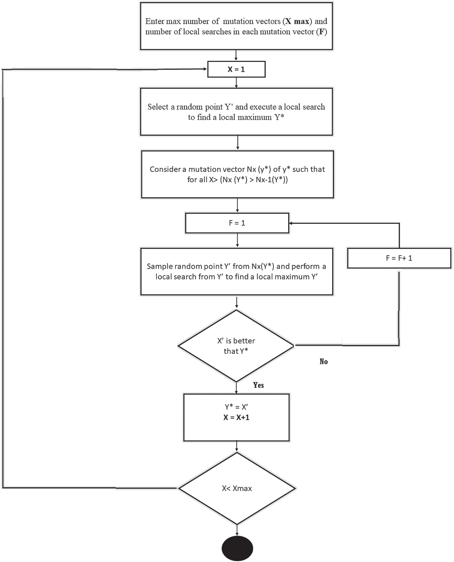
Figure 4: Flowchart of the proposed mutation mechanism
As aforementioned, this stage increases the vectors’ diversity by comparing the noisy random vector with the target vector to generate a trial vector. Eq. (3) is used to generate a trial vector with settings of rndb (n) and crossover ratio.
This stage achieves optimal DC selection by applying the rule mentioned in Section 3.4. The vector among trial and target vectors with the lowest fitness function value is selected as the next generation’s target vector.
Since real-world problems commonly contain computationally expensive objectives, the optimization iteration should finish as soon as the optimum solution is obtained. Several techniques are available to determine the best stopping criterion for evolutionary algorithms [31–33]. However, determining this stopping condition is not a simple task. While the global optimum is generally unknown, distance measures are not usable to achieve this goal. Stopping after a specific number of generations is limited to trial-and-error techniques that are used to determine the appropriate number of objective runs. Also, the number of objectives runs at which convergence happens is subject to large fluctuations because of the randomness in evolutionary algorithms. Subsequently, efficient stopping criteria must be applied to comply adaptively with the state of the optimization run. In this paper, a distribution-based criterion [33] called Diff, that depends on the difference between the value of the best objective function and the value of the worst objective function in a generation. The following rule is the termination condition used in this paper. If (Diff < Thr)
Terminate;
else
Proceed;
Where Thr denotes a value with many orders of magnitude less than the required accuracy of the optimum [34].
An experimental analysis proves that the convergence rate of 100% has been achieved when the difference threshold is set to one order of magnitude smaller than the demanded accuracy [33].
One hundred numerical experiments were conducted using two optimization methods to demonstrate the superiority of the modified DE over conventional DE. Fig. 5 illustrates the number of cases that each method can find the global maximum solution and how predominantly it ended up in the local maximum of the multi-objective function.
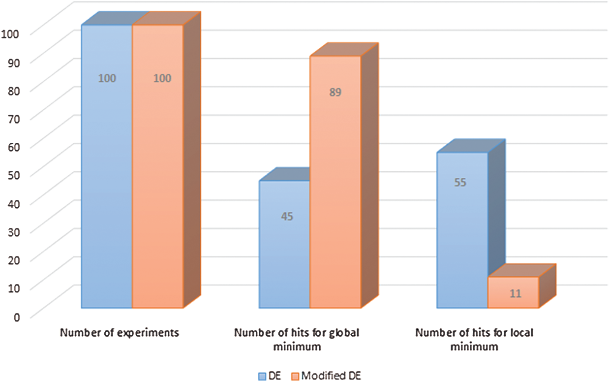
Figure 5: Experiments carried out using a modified and conventional DE
The modified DE algorithm is an extremely high global optimizer since it achieves an 89% hitting rate for the global maximum. Thus, it ensures getting asymptotic convergence to the global maximum.
This section provides details of the simulation environment and scenarios used in this paper and discusses the experiments and findings.
This section provides details of the simulator used in this paper and simulation scenarios as well.
The CloudAnalyst simulator is used to implement the proposed CSB policy and to simulate the experiments. It is easy to use due to its interactive graphical user interface, ability to configure simulation environment with a high degree of flexibility, and ability to provide visual and numerical outputs [35].
Six simulation scenarios are used to evaluate the proposed policy. Each scenario describes different situations regarding the number of cloud DC(s) and user bases that initiate jobs. Tab. 2 presents these simulation scenarios in detail.
The proposed HPLCCSB policy is evaluated with other existing CSB policies, including [25,35]: (i) closest DC policy, (ii) optimized response time policy (iii) reconfigure dynamically with load balancing policy, and (iv) OSBRP policy in terms of processing time, response time and total cost.
The experiments are performed five times for each scenario described earlier in Tab. 1. Each load balancing policy includes round-robin, equally spread load execution, and throttled load balancing policy to verify results and ensure more reliable and accurate findings to reflect the real world. The following sections report the overall findings and the proposed CSB policy’s evaluation against the existing CSB policy in terms of processing time, response time, and the total cost.
5.2.1 Evaluation of HPLCCSB Using Testing Scenarios
The following testing scenarios aim to assess the proposed HPLCCSB policy’s ability to select the most appropriate cloud DC to execute incoming users’ requests in the CC environment. Mainly, the evaluation focuses on calculating the processing and response time and the total cost of the proposed policy. Herein, the evaluation process is divided into six sub-scenarios to evaluate the HPLCCSB policy using the CloudAnalyst simulator.
All simulation scenarios were executed using the same configurations to get the most accurate results by covering both peak and off-peak hours to analyze the proposed HPLCCSB policy’s efficiency. Since the proper allocation of the CC resources is guaranteed during user request execution, an appropriate selection of CSB policy and load balancing policy should positively influence the overall CC environment’s QoS [24] and [35]. Each simulation scenario was executed five times for each load balancing policy (a total of 15 times) to ensure consistent CloudAnalyst simulator results and average performance metrics (i.e., response time, processing time, and total cost). The detailed results for the six simulation scenarios are in the following subsections.
Evaluation Using Simulation Scenario 1 The first scenario aims to determine the influence of low load on the performance metrics. Herein, the proposed HPLCCSB policy is evaluated by executing the first simulation scenario using round-robin, equally spread execution load, and throttled load balancing policies. Tab. 3 shows the obtained results.
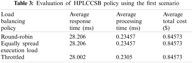
In this experiment, it is noticeable that the proposed HPLCCSB policy has improved performance since it always routes the different users’ requests to the cloud DCs with the best processing power. Therefore, it reduces congestion to the lowest level, unlike most existing CSB policies that might repeatedly select the same cloud DC to execute different user requests. The proposed HPLCCSB policy performs better with throttled load balancing policy because it assigns only one user’s request to each virtual machine at a time, and the other users’ requests can be routed to other virtual machines. Thus the proposed policy assures efficient execution of the users’ requests using different cloud DCs with minimal response, processing time, and total cost.
Evaluation Using Simulation Scenario 2 The second scenario aims to assess the influence of heavy load on the CC environment’s performance metrics. In a similar evaluation manner in scenario 1, the proposed policy is evaluated by executing the second simulation scenario using the three selected load balancing policies. Tab. 4 shows the findings resulted from the HPLCCSB policy using the second scenario.
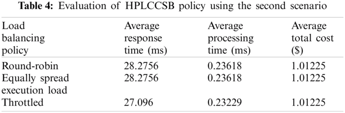
The results show a trivial decrease in the response time because of the slight reduction in the processing time compared to results when executing simulation scenario 1. Indeed, this trivial decrease is due to the large load rate on the available network and the cloud DCs. But the proposed policy still has improved performance because it ensures selecting the cloud DCs with the best processing power each time.
Evaluation Using Simulation Scenario 3 Simulation Scenario 3 aims to assess the influence of an increasing number of users’ requests per unit of time on the CC environment’s performance metrics. The proposed policy is evaluated using a similar evaluation mechanism followed previously by executing simulation scenario 3, and the results are in Tab. 5. The average total cost increases in this simulation scenario compared to scenario number 2 due to the number of users’ requests and the data transfer cost. But the response time and the processing time are not considerably impacted.
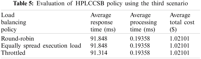
The experiment results demonstrate that out of the selected load balancing policies, the cloud DC response and processing time are the lowest when using the throttled policy. The response and processing time are low because the HPLCCSB policy ensures an efficient allocation of the users’ requests to all cloud DCs with the optimal processing power and ready to execute user requests. The throttled policy guarantees that each virtual machine has single user’s request to execute. This equitable allocation enhances the performance of the proposed HPLCCSB policy significantly.
Evaluation Using Simulation Scenario 4 Simulation Scenario 4 aims to assess the influence of peak and off-peak users’ parameters on the CC environment’s performance metrics. In this regard, the experimental results, shown in Tab. 6, ensure that the parameters that relate to the peak and off-peak users are important to bypass any influence on the response time or the processing time due to cloud changes DCs’ load.
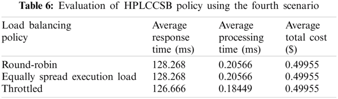
The proposed policy performs much better when executed with throttled load balancing policy. Hence, considering the DCPP parameter (i.e., the proposed fitness function) with throttled load balancing policy enhances the QoS requirements for the simultaneous online users during peak or off-peak hours. Therefore, the average number of dropped user requests is noticeably decreased, the average number of executed users’ requests is increased, and the average number of rejected users’ requests is also decreased (i.e., the DC efficiency is increased) with a reduced cost of VM usage.
Evaluation Using Simulation Scenario 5 The fifth scenario aims to assess the influence of the cloud DCs’ location from the user base on the CC environment’s performance metrics. This simulation scenario illustrates the worst-case scenario that the HPLCCSB policy might encounter due to the user bases’ geographical location and the cloud DCs. Despite that challenge, the proposed policy still achieves improved performance metrics (i.e., response and processing time and total cost). Tab. 7 presents the findings resulted from the HPLCCSB policy using the fifth scenario.
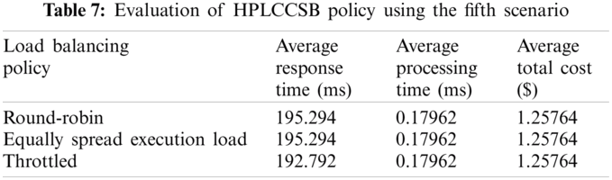
Also, the HPLCCSB policy performs much better when used with the throttled load balancing policy. The distribution of the cloud DC among different regions might negatively affect the data transfer cost (i.e., total cost). However, using the proposed CSB policy with the throttled load balancing policy might reduce the required data transfer cost by utilizing the most efficient cloud DC and VM among the available resources.
Evaluation Using Simulation Scenario 6 Finally, similar to simulation scenario 5, the aim of simulation scenario 6 is to assess the influence of the geographical location of the cloud DCs and user bases on the performance metrics in the CC environment. This simulation scenario proves the urgent need for such a policy that accommodates different situations by routing users’ requests to different cloud DCs only when required. Since many distributions of users’ requests among DCs will not always be the optimal solution, the proposed HPLCCSB policy selects a smaller number of cloud DCs for user request execution. It selects a new cloud DC only if needed. Therefore, the response time decreased noticeably. Tab. 8 presents the results from the HPLCCSB policy using the sixth scenario.
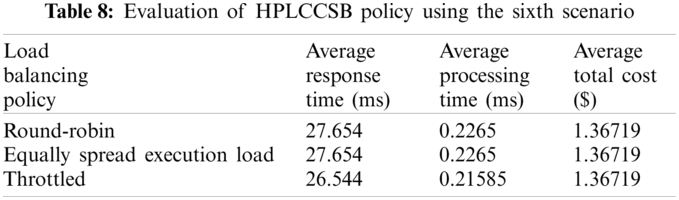
The results in Tab. 8 show a considerable reduction in the cloud DCs’ response time when using simulation scenario number 6. It requires less processing time obtained from executing the previous simulation scenario compared to this simulation scenario. Indeed, it is deduced that the processing time in every cloud DC is minimized once the user base is situated in a totally different region from the cloud DC.
5.2.2 Comparative Analysis with Existing CSB Policies
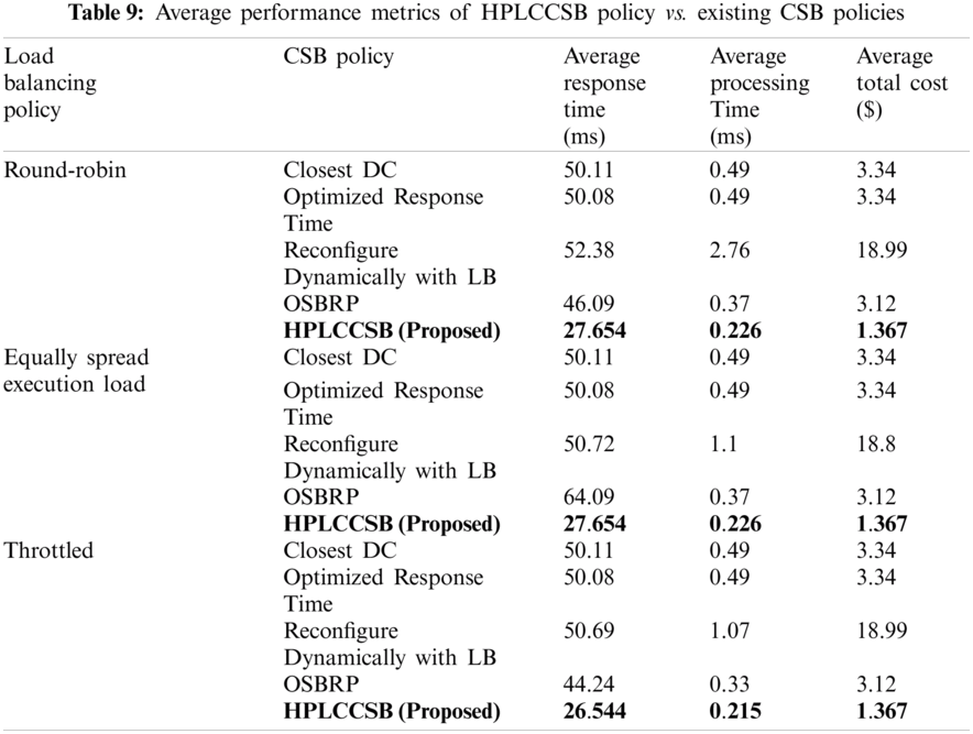
The performance of the proposed HPLCCSB policy is compared with some of the well-known CSB policies based on the evaluation metrics that are obtained from the previous simulation scenarios. The comparative test is used to estimate the computation time and total cost of the proposed HPLCCSB policy against related CSB policies for selecting the cloud DCs in the CC computing environment (refer to Fig. 8). The proposed HPLCCSB policy is compared with the closest DCs, the optimized response time, the reconfigure dynamically with load balancing, and the OSBRP policies for the following reasons: (i) The closest DC policy is one of the simplest DC selection technique in the CC environment, (ii) The optimized response time policy achieves superb response time, (iii) The reconfigure dynamically with load balancing policy has a varied behavior according to simulation scenario, which might perform more suitable in specific scenarios, (iv) The OSBRP policy is based on a metaheuristic optimization algorithm similar to the proposed policy. Tab. 9 shows the average of evaluation metrics of HPLCCSB Policy vs. existing CSB policies.
In specific, the findings demonstrated in Tab. 9 reveal that out of the three selected virtual machine load balancing policies, the average response time, the average processing time, and the average total cost are the lowest when using Throttled policy with the proposed HPLCCSB policy. As aforementioned, this fact is due to the HPLCCSB policy guarantees an efficient allocation of users’ requests to all the cloud DCs that have the best processing power and available for executing the users’ requests. In comparison, the throttled load balancing policy guarantees that each virtual machine has only one user request for execution. This balanced and efficient distribution of users’ requests enhances response and processing time substantially.
5.2.3 Significance of Enhancement
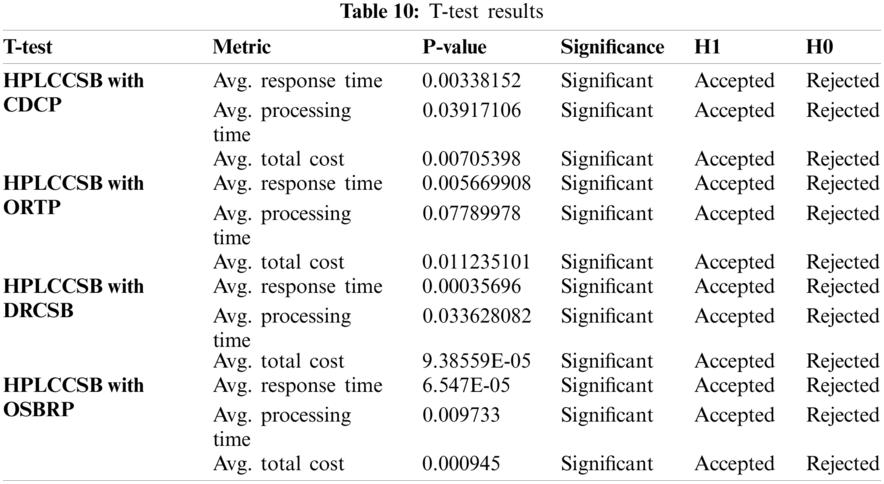
This section is to measure whether the enhancement produced by HPLCCSB is significant or not using the T-test. A T-test is one of the most commonly used statistical tests to compare means [36]. It is a parametric technique where the probability distribution of variables is defined, and inferences about the distribution parameters are made. The T-test is usually used when two independent groups describe the experimental subjects. It is also known as a student’s T-test, which can be used as a statistical analysis method to test whether there is a difference between two independent means or not.
However, statistical significance is measured by calculating the probability of error (i.e., the p-value). If p is less than 0.05, the difference between the two means is statistically significant; else, the difference is not significant. Therefore, in this paper, the hypothesis of significance can be formulated as follows:
H0: HPLCCSB does not significantly enhance the other CSB policies with respect to evaluation metrics.
H1: HPLCCSB does significantly enhance the other CSB policies with respect to evaluation metrics.
Tab. 10 summarizes the T-test results, while Figs. 6 and 7 presents the enhancement percentages of HPLCCSB with CDCP, ORTP, DRCSB, and OSBRP in average processing time, average response time, and average total cost, respectively. However, the results show that the proposed HPLCCSB policy has significantly improved the other existing CSB policies in terms of average processing time, average response time, and average total cost.
In sum, HPLCCSB enhances the average processing time of CDCP, ORTP, DRCSB, and OSBRP by 48.12%, 47.2%, 84.8%, and 37%, respectively, when using a round-robin load balancing policy. When using the equally spread execution-load load balancing policy, the HPLCCSB enhances the CDCP, ORTP, DRCSB, and OSBRP by 48.1%, 47.2%, 78%, and 37%, respectively. Using the throttled load balancing policy enhances CDCP, ORTP, DRCSB, and OSBRP by 49.7%, 48.9%, 78.7%, and 34.2%, respectively. While, in terms of the average response time, HPLCCSB also enhances CDCP, ORTP, DRCSB, and OSBRP by 50.5%, 50.4%, 54.1%, and 40%, respectively when using the round-robin load balancing policy. Besides, it enhances CDCP, ORTP, DRCSB, and OSBRP by 50.5%, 50.4%, 50.6%, and 40%, respectively, when using the equally spread execution-load load balancing policy. Moreover, HPLCCSB also enhances CDCP, ORTP, DRCSB, and OSBRP by 50.8%, 50.8%, 51%, and 39.5%, respectively, when using throttled load balancing policy. Also, in terms of the average total cost, the HPLCCSB enhances CDCP, ORTP, DRCSB, and OSBRP by 63.4%, 63.4%, 91.7%, and 56.1%, respectively when using a round-robin load balancing policy. Also, it enhances the CDCP, ORTP, DRCSB, and OSBRP by 63.3%, 63.3%, 91.7%, and 56.1%, respectively, when using the equally spread execution-load load balancing policy. Furthermore, when using the throttled load balancing policy, the HPLCCSB enhances CDCP, ORTP, DRCSB, and OSBRP by 63.3%, 63.3%, 91.7%, and 56.1%, respectively.
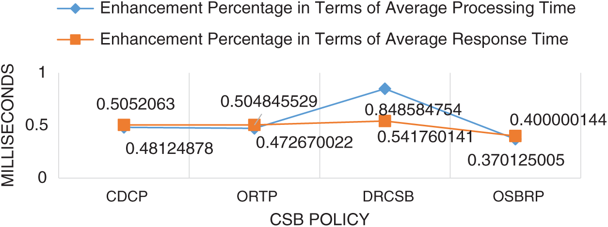
Figure 6: Enhancement percentages of HPLCCSB with other CSB policies using round-robin load balancing policy in terms of average processing time and average response time
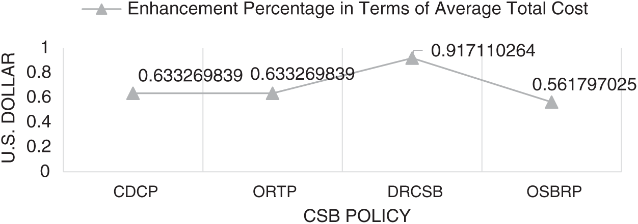
Figure 7: Enhancement percentages of HPLCCSB with other CSB policies using round-robin load balancing policy in terms of the average total cost
The effectiveness of the HPLCCSB has been demonstrated with three different load balancing policies: (i) round-robin, (ii) equally spread execution-load, and (iii) throttled. The HPLCCSB was evaluated using three main metrics: (i) average response time, (ii) average processing time, and (iii) average total cost. The following subsections discuss the results.
Average Processing Time and Average Response Time The previous section analysis reveals that the proposed HPLCCSB policy significantly improves the existing CSB policies’ performance in response and processing time. Since the HPLCCSB policy always routes the incoming user request to the least congested DC with maximum availability and efficiency and with the lowest average processing time and average response time, this might be guaranteed by maximizing the value of the proposed multi-objective function. Tab. 9 shows the comparison results, which reveal that the HPLCCSB has an average processing time of 0.212688 milliseconds, 0.212688 milliseconds, and 0.206066 milliseconds when using round-robin, equally spread execution-load, and throttled load balancing policies, respectively. In user requests executions, the average response time is 83.2576 milliseconds, 83.2576 milliseconds, and 82.069 milliseconds when using the round-robin, equally spread execution-load, and throttled load balancing policies, respectively. HPLCCSB has a lower average processing time because it routes user requests to the most efficient DC based on the processing power (i.e., the proposed multi-objective function). Consequently, this causes the users’ requests to be distributed to multiple DCs with the highest DCPP value, resulting in a significant reduction in response time and processing time.
By contrast, the existing CSB policies rely only on the previous DC load or processing time for the last executed user request, regardless of the expected processing time that might reflect the actual processing time to some extent. Besides, the HPLCCSB policy ensures efficient resource utilization by selecting the most suitable DC without overloading one DC over others. It always invokes more VMs on different DCs compared to other existing policies. The existing policies select the same DCs frequently, which overload them and increase the response and processing time. Therefore, giving high weight to DCEff (i.e., maximization-positive weight) ensures the selection of DC with minimal processing time and response time.
Due to the proposed MOF’s nature, HPLCCSB must achieve the minimum value of response time and processing for user request execution since it is one of the proposed MOF’s core objectives. Therefore, average processing time and average response time are compared with a minimum value of processing time and minimum value of response time, respectively, achieved by HPLCCSB using simulation scenarios. Figs. 8 and 9 depict comparison results of HPLCCSB with CDCP, ORTP, DRCSB, and OSBRP, respectively, by presenting the difference between minimum values and average values resulting from each CSB policy in terms of processing time and response time.
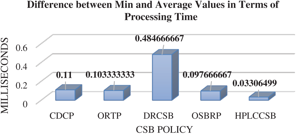
Figure 8: Difference between the minimum and average values for each CSB policy in terms of processing time using Round-Robin load balancing policy
Figs. 8 and 9 show the differences between the average values and minimum values of processing time and response time for each CSB policy. Since the HPLCCSB has the minimum difference between the value of average processing time and obtained value of minimum processing time and between the value of average response time and obtained value of minimum response time, thereby suggesting the HPLCCSB policy obtains the minimum processing time and response time values in the majority of the simulation experiments. By contrast, the difference between the average processing time and processing time’s minimum values, and the average response time and response time’s minimum values of the CDCP, ORTP, DRCSB, and OSBRP policies are mostly large. This large difference in the values indicate that these policies have higher processing time and response time in most of the experiments than the HPLCCSB policy. In sum, the HPLCCSB policy demonstrates optimal QoS requirements in terms of average processing time and average response time amongst these CSB policies.
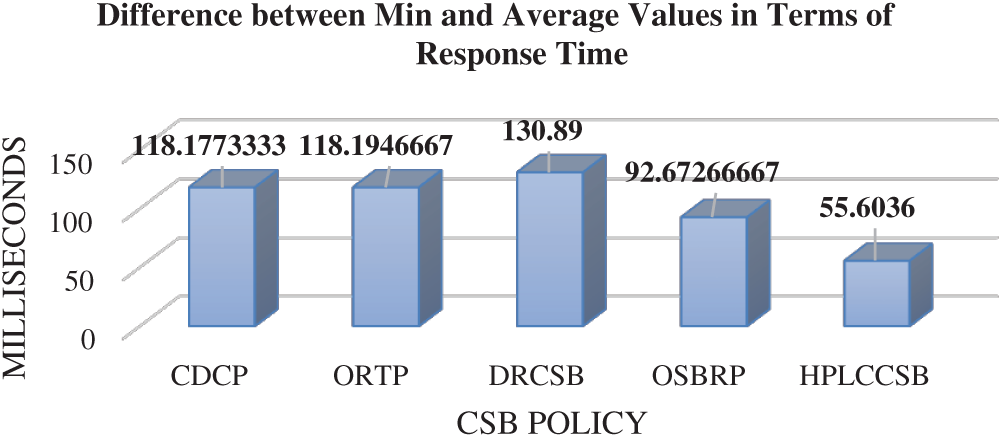
Figure 9: Difference between the minimum and average values comparison for each CSB policy in terms of response time using Round-Robin load balancing policy
Average Total Cost Unlike other existing CSB policies, the increase in the number of user requests or their sizes does not negatively impact HPLCCSB policy since it considers the incoming user requests sizes during DC selection (i.e., by considering the expected processing time in MOF). Additionally, it always execute user requests using the most efficient and available DC (i.e., DC with the highest value of DCEff and DCAV) among the existing DCs. Generally, executing large-sized user requests costs more than the small ones since it involves more data transfer between the DC and user base. Despite that, the HPLCCSB policy does not always increase the total cost significantly since it gives the highest weight (i.e., minimization-negative weight) to the total cost in the proposed MOF (refer to Tab. 9); thus, it ensures the lowest cost even when executing incoming user requests constantly. Meanwhile, the comparison results shown earlier in Tab. 9 reveal that HPLCCSB consumes less average total cost (1.000562 US Dollar, 1.000562 US Dollar, and 1.000562 US Dollar when using round-robin, equally spread execution-load, and throttled load balancing policies, respectively). Due to the proposed MOF’s nature, HPLCCSB must achieve the minimum value of total cost when executing user requests since it is one of the proposed MOF’s core objectives. Therefore, the average total cost is compared with the minimum value of total cost achieved by HPLCCSB using simulation scenarios. Fig. 10 shows the comparison of HPLCCSB with CDCP, ORTP, DRCSB, and OSBRP, respectively, by presenting the difference between minimum values and average values resulting from each CSB policy in terms of the total cost using a round-robin load balancing policy.
As noticed from the previous Fig., HPLCCSB has the minimum difference between average total cost and minimum obtained value of total cost, thereby suggesting that the HPLCCSB policy achieved the minimum total cost value in most simulation experiments. By contrast, the difference between values of average total cost and minimum values resulting from CDCP, ORTP, DRCSB, and OSBRP are mostly higher than the difference resulting from HPLCCSB, indicating that these policies have higher total cost values in most of the experiments. Therefore, the HPLCCSB policy demonstrates optimal QoS requirements in terms of average total cost amongst these CSB policies.
Due to the nature of the CC environment, based on a pay-as-you-go or pay-per-use basis, achieving minimum total cost is a major QoS requirement for cloud users. Therefore, from a cloud user’s perspective, HPLCCSB ensures executing their requests efficiently with minimum cost. From a security perspective, HPLCCSB minimizes the Economic Denial of Sustainability attack (EDoS) impact. Indubitably, understanding the reasoning behind scheduling decisions is quite important property in practical scenarios. In this regard, simple heuristics such as CDCP and ORTP are appealing approaches since the reason behind their scheduling decisions (the assignment of cloud applications to data centers) is straightforward. Any alternative scheduling decisions approach must have significant performance improvements to be appealing. In this context, results of enhancement significance justify the need for the deployment of the proposed policy since it performs better when compared to simple heuristics.
In conclusion, the HPLCCSB policy is usable to select the most appropriate DC in the cloud environment to execute the users’ requests efficiently without degrading the level of QoS. Implementing the proposed CSB policy in a real-cloud environment might ensure efficient selection of the DCs without being overloaded; thereby, improving the overall performance and reducing the total cost. Therefore, efficient utilization of the DCs enhances the cloud environment by allowing user request execution with a high QoS level. Indeed, the HPLCCSB policy achieves the major QoS requirements, including the lowest processing time, lowest response time, and minimum total cost. This policy also provides a better QoS than CDCP, ORTP, DRCSB, and OSBRP in terms of average processing time, average response time, and average total cost.
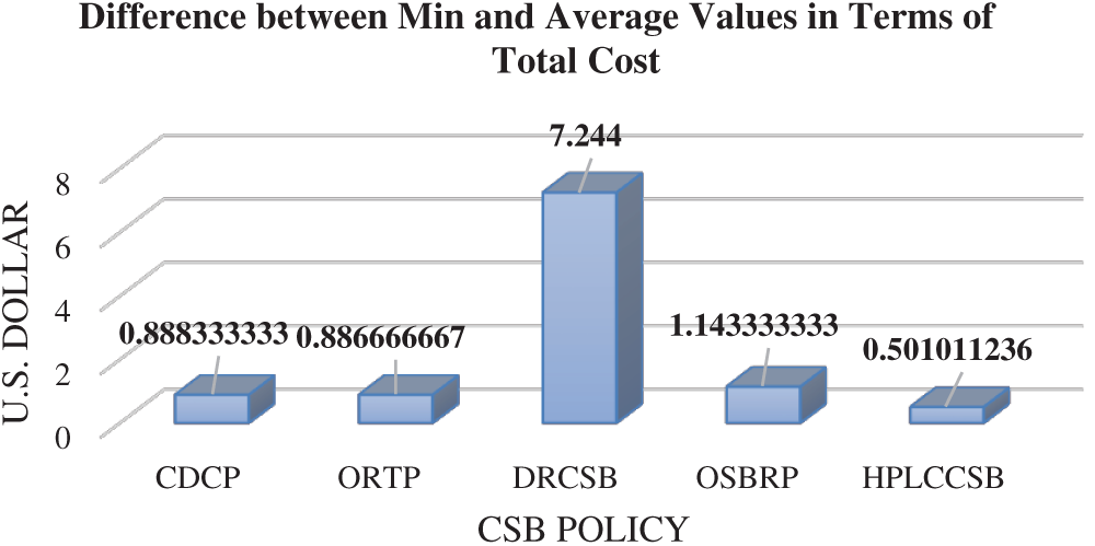
Figure 10: Difference between the minimum and average values for each CSB policy in terms of the total cost using Round-Robin load balancing policy
This paper proposed a modified DE algorithm-based CSB policy used to select the cloud DC. The attention to finding an efficient CSB policy to select the cloud data center is always a topic of interest due to the continuous growth of users’ requests. As reviewed from prior works, traditional and existing proposed CSB policy still suffer from different challenges due to the dynamic and incremental nature of users’ requests. Compared to the existing policies, the proposed policy using a modified DE algorithm seems a practicable policy to route users’ requests to the most efficient DC. The findings demonstrate that the proposed policy is superior to other existing policies.
As future work, the cloud users’ QoS requirements should be considered to determine how good the solution is with respect to the optimal solution. Besides, deploying the proposed solution in an online mode (i.e., real cloud’s environment) should take place in the future to determine the ability of the proposed solution in dealing with varying arrival rates of real users’ requests.
Acknowledgement: I express my gratitude to Universiti Sains Malaysia, Malaysia and Northern Border University, Saudi Arabia, for administrative and technical support.
Funding Statement: This work was supported by Universiti Sains Malaysia under external grant (Grant Number 304/PNAV/650958/U154).
Conflict of Interest: The authors declare that they have no conflicts of interest to report regarding the present study.
1. D. Abts and B. Felderman, “A guided tour through data-center networking,” Queue, vol. 10, no. 5, pp. 10–23, 2012. [Google Scholar]
2. H. Qi, M. Shiraz, J. Liu, A. Gani, Z. Rahman et al., “Data center network architecture in cloud computing: Review, taxonomy, and open research issues,” Journal of Zhejiang University Science, vol. 15, no. 9, pp. 776–793, 2014. [Google Scholar]
3. Cisco, Cisco Global Cloud Index 2015–2020, 2016. [Online]. Available: https://www.cisco.com/c/dam/m/en_us/service-provider/ciscoknowledgenetwork/files/622_11_15-16-Cisco_GCI_CKN_2015-2020_AMER_EMEAR_NOV2016.pdf. [Google Scholar]
4. R. Naha and M. Othman, “Cost-aware service brokering and performance sentient load balancing algorithms in the cloud,” Journal of Network and Computer Applications, vol. 75, no. 23, pp. 47–57, 2016. [Google Scholar]
5. A. Jaikar and S. Noh, “Cost and performance effective data center selection system for scientific federated cloud,” Peer-to-Peer Networking and Applications, vol. 8, no. 5, pp. 896–902, 2015. [Google Scholar]
6. A. Manasrah, T. Smadi and A. ALmomani, “A variable service broker routing policy for data center selection in cloud analyst,” Journal of King Saud University-Computer and Information Sciences, vol. 29, no. 3, pp. 365–377, 2017. [Google Scholar]
7. A. Amairah, B. Al-tamimi, M. Anbar and K. Aloufi, “Cloud computing and internet of things integration systems: A review,” in Int. Conf. of Reliable Information and Communication Technology, Springer, Cham, Pahanag, Malaysia, pp. 406–414, 2019. [Google Scholar]
8. D. Arya and M. Dave, “Priority based service broker policy for fog computing environment,” in Int. Conf. on Advanced Informatics for Computing Research, Springer, Singapore, pp. 84–93, 2017. [Google Scholar]
9. A. Hurson and H. Sarbazi-Azad, “Energy Efficiency in Data Centers and Clouds,” San Diego, CA, USA: Elsevier, 2016. [Online]. Available: https://www.elsevier.com/books/energy-efficiency-in-data-centers-and-clouds/hurson/978-0-12-804778-1. [Google Scholar]
10. L. Rao, X. Liu, L. Xie and W. Liu, “Minimizing electricity cost: optimization of distributed internet data centers in a multi-electricity-market environment,” in Proc. IEEE INFOCOM, San Diego, CA, USA, 2010, pp. 1–9, 2010. [Google Scholar]
11. M. Sharkh, A. Kanso, A. Shami and P. Öhlén, “Building a cloud on earth: A study of cloud computing data center simulators,” Computer Networks, vol. 108, no. 17, pp. 78–96, 2016. [Google Scholar]
12. S. Shetty, X. Yuchi and M. Song, “Optimizing network-aware resource allocation in cloud data centers,” in Moving Target Defense for Distributed Systems, Springer, Guangzhou, China, pp. 43–55, 2016. [Google Scholar]
13. V. Reddy, G. Gangadharan, G. Rao and M. Aiello, “Energy-Efficient Resource Allocation in Data Centers Using a Hybrid Evolutionary Algorithm,” in Machine Learning for Intelligent Decision Science, Springer, Singapore, pp. 71–92, 2020. [Google Scholar]
14. M. Klinkowski, K. Walkowiak and R. Goścień, “Optimization algorithms for data center location problem in elastic optical networks,” in 2013 15th Int. Conf. on Transparent Optical Networks, IEEE, Cartagena, Spain, pp. 1–5, 2013. [Google Scholar]
15. V. Sharma, R. Rathi and S. Bola, “Round-robin data center selection in single region for service proximity service broker in cloudAnalyst,” International Journal of Computers & Technology, vol. 4, no. 21, pp. 254–260, 2013. [Google Scholar]
16. Z. Benlalia, A. Beni-hssane, K. Abouelmehdi and A. Ezati, “A new service broker algorithm optimizing the cost and response time for cloud computing,” Proc. Computer Science, vol. 151, no, 11, pp. 992–997, 2019. [Google Scholar]
17. D. Zou, H. Liu, L. Gao and S. Li, “A novel modified differential evolution algorithm for constrained optimization problems,” Computers & Mathematics with Applications, vol. 61, no. 6, pp. 1608–1623, 2011. [Google Scholar]
18. A. Mohamed and A. Mohamed, “Adaptive guided differential evolution algorithm with novel mutation for numerical optimization,” International Journal of Machine Learning and Cybernetics, vol. 10, no. 2, pp. 253–277, 2019. [Google Scholar]
19. S. Wang and H. Yang, “Self-adaptive mutation differential evolution algorithm based on particle swarm optimization,” Applied Soft Computing, vol. 81, no. 7, pp. 1723–1741, 2019. [Google Scholar]
20. R. Storn and K. Price, “Differential evolution–a simple and efficient heuristic for global optimization over continuous spaces,” Journal of Global Optimization, vol. 11, no. 4, pp. 341–359, 1997. [Google Scholar]
21. S. Das and P. Suganthan,“Differential evolution: A survey of the state-of-the-art,” IEEE Transactions on Evolutionary Computation, vol. 15, no. 1, pp. 4–31, 2011. [Google Scholar]
22. J. Zhang and A. Sanderson, “JADE: Adaptive differential evolution with optional external archive,” IEEE Transactions on Evolutionary Computation, vol. 13, no. 5, pp. 945–958, 2009. [Google Scholar]
23. D. Karaboğa and S. Ökdem, “A simple and global optimization algorithm for engineering problems: Differential evolution algorithm,” Turkish Journal of Electrical Engineering & Computer Sciences, vol. 12, no. 1, pp. 53–60, 2004. [Google Scholar]
24. B. Wickremasinghe and R. Buyya, “Cloudanalyst: A cloudSim-based tool for modelling and analysis of large-scale cloud computing environments,” MEDC Project Report, vol. 22, no. 6, pp. 433–659, 2009. [Google Scholar]
25. A. Manasrah and B. Gupta, “An optimized service broker routing policy based on differential evolution algorithm in fog/cloud environment,” Cluster Computing, vol. 21, no. 11, pp. 1–15, 2018. [Google Scholar]
26. N. Kofahi, T. Alsmadi, M. Barhoush and A. Moy’awiah, “Priority-based and optimized data center selection in cloud computing,” Arabian Journal for Science and Engineering, vol. 44, no. 11, pp. 9275–9290, 2019. [Google Scholar]
27. N. Gunantara, N. Sastra and G. Hendrantoro, “Cooperative diversity path pairs selection protocol with multi objective criterion in wireless ad hoc networks,” International Journal of Applied Engineering Research, vol. 9, no. 23, pp. 417–426, 2014. [Google Scholar]
28. N. Gunantara, “A review of multi-objective optimization: Methods and its applications,” Cogent Engineering, vol. 5, no. 1, pp. 150–224, 2018. [Google Scholar]
29. H. Einhorn and W. McCoach, “A simple multiattribute utility procedure for evaluation,” Behavioral Science, vol. 22, no. 4, pp. 270–282, 1977. [Google Scholar]
30. K. Parsopoulos, “UPSO: A unified particle swarm optimization scheme,” Lecture Series on Computer and Computational Science, vol. 1, no. 13, pp. 868–873, 2004. [Google Scholar]
31. K. Zielinski, D. Peters and R. Laur, “Run time analysis regarding stopping criteria for differential evolution and particle swarm optimization,” in Proc. of the 1st Int. Conf. on Experiments/Process/System Modelling/Simulation/Optimization, Athens, Greece, pp. 215–224, 2005. [Google Scholar]
32. K. Zielinski, P. Weitkemper, R. Laur and K. Kammeyer, “Examination of stopping criteria for differential evolution based on a power allocation problem,” in Proc. of the 10th Int. Conf. on Optimization of Electrical and Electronic Equipment, Braşov, Romania, pp. 149–156, 2006. [Google Scholar]
33. K. Zielinski and R. Laur, “Stopping criteria for differential evolution in constrained single-objective optimization,” in Advances in Differential Evolution, Springer, Berlin, Heidelberg, pp. 111–138, 2008. [Google Scholar]
34. K. Price, R. Storn and J. Lampinen, “Differential evolution: A practical approach to global optimization,” in Springer In Science & Business Media, 1st ed., vol. 1. Berlin, Germany: Advances in Optimization Press, pp. 31–397, 2006. [Google Scholar]
35. B. Wickremasinghe, R. Calheiros and R. Buyya, “Cloudanalyst: A cloudsim-based visual modeller for analysing cloud computing environments and applications,” in 24th IEEE Int. Conf. on Advanced Information Networking and Applications, Perth, WA, Australia, pp. 446–452, 2010. [Google Scholar]
36. T. Kim, “T test as a parametric statistic,” Korean Journal of Anesthesiology, vol. 68, no. 6, pp. 540–551, 2015. [Google Scholar]
 | This work is licensed under a Creative Commons Attribution 4.0 International License, which permits unrestricted use, distribution, and reproduction in any medium, provided the original work is properly cited. |