DOI:10.32604/cmc.2021.018872
| Computers, Materials & Continua DOI:10.32604/cmc.2021.018872 | |
| Article |
Modeling CO2 Emission of Middle Eastern Countries Using Intelligent Methods
1Sustainable and Renewable Energy Engineering Department, University of Sharjah, PO Box 27272, Sharjah, UAE
2College of Engineering and Technology, American University of the Middle East, Kuwait
3Department of Mechanical and Industrial Engineering, Louisiana State University, USA
*Corresponding Author: Ibrahim Mahariq. Email: ibrahim.maharik@aum.edu.kw
Received: 23 March 2021; Accepted: 24 April 2021
Abstract: CO2 emission is considerably dependent on energy consumption and on share of energy sources as well as on the extent of economic activities. Consequently, these factors must be considered for CO2 emission prediction for seven middle eastern countries including Iran, Kuwait, United Arab Emirates, Turkey, Saudi Arabia, Iraq and Qatar. In order to propose a predictive model, a Multilayer Perceptron Artificial Neural Network (MLP ANN) is applied. Three transfer functions including logsig, tansig and radial basis functions are utilized in the hidden layer of the network. Moreover, various numbers of neurons are applied in the structure of the models. It is revealed that using MLP ANN makes it possible to accurately predict CO2 emission of these countries. In addition, it is concluded that using logsig transfer function leads to the highest accuracy with minimum value of mean squared error (MSE) which is followed by the networks with radial basis and tansig transfer functions. The R-squared of the networks with logsig, radial basis and tansig transfer functions are 0.9998, 0.9997 and 0.9996, respectively. Finally, comparison of the proposed model with a similar study, considered five countries in the same region, reveals higher accuracy in term of MSE.
Keywords: CO2 emission; artificial neural network; middle eastern countries; transfer function
Climate change is one of the main concerns of scientists working on the environment due to its detrimental effects such as shrinkage in glaciers, change in animal and plant ecosystem, heat waves with higher intensity, sea level rise, etc. [1,2]. Greenhouse gases highly influence the climate change [3], which necessitates utilizing different approaches, fuels, energy sources and alternatives to mitigate their emission [4,5]. CO2 is one of the greenhouse gases that is mainly emitted by energy consumption and through the relevant industries and technologies [6]. Due to its harmful effects, considerable efforts have been made to decrease CO2 emission so far. Enhancing the efficiency of the current energy systems and developing clean energy systems are the main solutions to hinder this situation [7,8]. In order to have deep insight into the CO2 emission, it is required to model it. In this regard, employing Artificial Intelligence would be a practical approach. However, it is vital to use a reliable model through appropriate inputs; therefore, all of the influential elements must be considered.
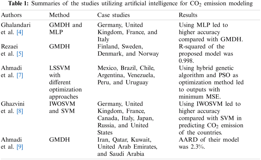
Artificial Intelligence is an efficient approach for modeling and predicting complex system with different effective factors [9,10]. Methods based on artificial intelligence, such as artificial neural network (ANN), have been broadly applied in different fields of science such as medical, engineering and management [11–13]. Owing to their efficient performance in forecasting the outputs of the systems, they can be applied for predicting complex situations. Various studies have applied these methods for predicting CO2 emission for different countries. For instance, Ghalandari et al. [14] used multilayer perceptron (MLP) and Group Method of Data Handling (GMDH) for CO2 emission of four countries located in Europe. They concluded that CO2 emission can be forecasted with great accuracy, with R-squared value of around 0.9999. In another work [15], GMDH was used for the same purpose in four Nordic countries. The proposed model was remarkable with R-squared of 0.998. Ahmadi et al. [16] applied Least Square Support Vector Machine (LSSVM) as an intelligent approach for predicting CO2 emission of six American Latin countries and found that this method has excellent performance for their purpose. According to these works, it can be concluded that these techniques would be leading for CO2 emission modeling. In Tab. 1, summaries of the research studies that applied Intelligent Methods for CO2 emission modeling are provided.
In the Middle East, renewable energy-based technologies have not been developed greatly due to the abundance of different types of fossil fuels. Owing to this fact, CO2 emissions of these countries are relatively high in comparison with their industrial activities and population. Although there are some limited research focusing on utilization of intelligent methods for CO2 emission for different countries, there is only one study on the Middle Eastern countries [19]. In this regard, this work concentrates on proposing a predictive model for CO2 emission in seven Middle Eastern countries including Iran, United Arab Emirates, Qatar, Kuwait, Saudi Arabia, Turkey and Iraq. In comparison with the mentioned study on the Middle Eastern countries, the present paper includes more case studies. Furthermore, the applied method, i.e., MLP ANN, has shown superior performance in predicting CO2 emission. To propose a model with maximum possible accuracy, MLP with different architectures and transfer functions are used in this work. Moreover, the accuracy of the models is compared based on statistical criteria. In the next section of this article, the case studies are introduced based on their energy consumption and CO2 emission; afterwards, the applied method is explained. Subsequently, in the fourth section, results are represented and discussed. Finally, in conclusion section, the main findings of this study are provided.
In this paper, seven Middle Eastern countries are considered as case studies for modeling of CO2 emissions. In this part, some of the most important data about these countries are presented. The first one is Iran, which is located in the west of Asia with a population of 82,913,000 in 2019 [20]. Iran's primary energy consumption has increased from 3.04 EJ in 1990 to around 12.34 EJ in 2019. In this period, CO2 emission has increased from around 190.6 Mt to more than 670 Mt [21]. Several policies, such as supporting cooperative and private sectors to facilitate installing renewable energy technologies [22] have been made and implemented in this country in recent years to decrease CO2 emission. The next country considered here as a case study is Iraq. This country locates in the west of Asia and is known as one of the important oil exporters. Its population was around 39,309,000 in 2019 [20]. CO2 emission of Iraq has increased from 52.3 Mt in 1990 to around 148 Mt in 2019. In the same period, its primary energy consumption has increased from 0.82 EJ to 2.23 EJ [21]. Some policies, like undertaking pollution treatment via applying clean technologies for polluting activities [22] have been designed to reduce CO2 emission and reach more appropriate qualities in term of environment. Kuwait, located in the west of Asia, is the next in the list and is considered here for modeling its CO2 emission. Kuwait is one of the resource-reach countries that exports crude oil in large extent, i.e., more than 102 Mt in 2019 [22]. Its population in 2019 was around 4,207,000 [20] and its CO2 emission has increased from 18.4 Mt in 1990 to around 97.3 Mt in 2019. In this period, Kuwait's total primary energy consumption has grown from around 0.29 EJ to about 1.64 EJ [21]. Kuwait has invested on development of renewable energy technologies in recent years to improve the diversity of its energy systems making it more environmentally friendly. United Arab Emirates (UAE) is another Middle Eastern country in the west of Asia with population of around 9,770,000 in 2019 [20]. Its primary energy consumption has increased from 1.25 EJ to about 4.83 EJ between 1990 and 2019. In this period, its CO2 emissions has grown from 82.2 Mt to 282.6 Mt [21]. UAE has invested in renewable energies, especially solar, in recent years which would result in lower emission of CO2 per unit of energy consumption. Saudi Arabia is another case study of the present work which is located in the South West of Asia. This country has a key role in supplying world crude oil by exporting it in large extent. The population of Saudi Arabia in 2019 was around 34,268,000 [20]. Its primary energy consumption has been increased from around 3.34 EJ to about 11.04 EJ between 1990 and 2019. During these years, its CO2 emission has grown from about 202.3 Mt to around 579.9 Mt [21]. Saudi Arabia has invested in various clean energy technologies such as renewable energy-based desalination systems and power generation. Moreover, this country aims to reach a leading researcher position in field of energy [22]. Qatar, located in west of Asia, with population of around 2,832,000 in 2019 [20] occupies the second place of natural gas export in the world. CO2 emission of Qatar has increased from around 14.2 Mt to about 102.5 Mt from 1990 to 2019. In this period, its primary energy consumption has increased from approximately 0.31 EJ to around 2.02 EJ [21]. In order to reach sustainable development, this country has proposed several programs in recent years that cover various aspects such as setting standard values for energy technologies [22]. Turkey is the only European country that is considered in this study. It is located in the South Eastern of Europe and west of Asia with population of around 83,429,000 in 2019 [20]. In the mentioned time period for the previous countries, the primary energy consumption of Turkey has increased from approximately 2.01 EJ to about 6.49 EJ. In this period, its CO2 emission has increased from around 136.2 Mt to around 383.3 Mt [21]. Several energy-related policies, such as developing nearly zero energy building have been applied in this country to improve energy efficiency and decrease the related environmentally harmful effects [22].
In Fig. 1, average annual growth of primary energy consumption and CO2 emission between 1990 and 2019 are illustrated. As shown in this figure, average annual growth of both mentioned parameters are maximum for Qatar between 1990 and 2019 among the considered case studies. In addition to the case studies, these factors are compared with the corresponding values of the world and OECD countries to get a better insight. It can be concluded that growth in CO2 emission and primary energy consumption of the considered countries for the present study are higher compared to that in the world as well as OECD countries. That can be attributed to a lower share of renewable energies and relatively lower efficiency of energy technologies. As shown in Fig. 2, share of renewable energies in the countries considered for modeling, except Turkey, is much lower compared to that in the world and OECD countries. By considering all countries, the share of renewables in primary energy consumption is around 3.81%, while it is around 12.45% and 11.4% for OECD countries and the world; respectively.
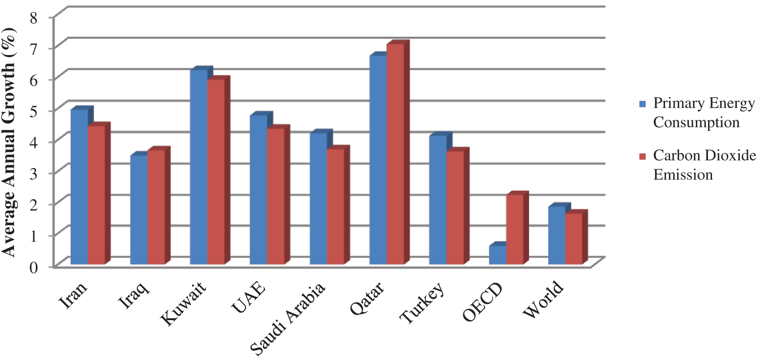
Figure 1: Average annual growth in primary energy consumption and carbon dioxide emission between 1990 and 2019 [21]
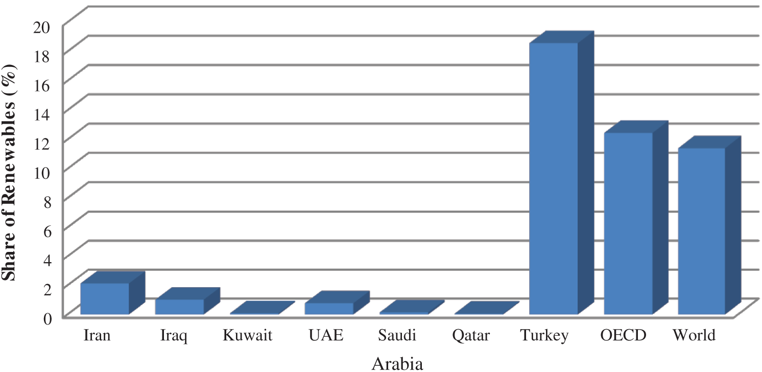
Figure 2: Share of renewable energies in primary energy consumption in 2019 [21]
Multilayer perceptron (MLP) ANN is employed here for modeling and predicting CO2 emission of the considered countries. MLP is one of the common methods in artificial neural networks. Its working procedure is depicted in Fig. 3. This approach is built on three base layers which are called input layers, hidden layer and output layer and the mentioned layers are in control of locating the input data, processing the data, and representing the outcome, respectively. It is worth mentioning that this method benefits from numerous nodes that are connected through a weight vector in each of the aforementioned layers. The nodes in input layer collect the data and process them in the hidden layer and show them in the result layer. The collected information by the nodes in the input layer is combined for the next layer's nodes. The connection between the input vector, weight vector, nodes and the transfer function f of the summation of input nodes to the hidden layer are presented as [23,24]:
where K, θj and ωji describe the amounts of hidden layers, the threshold of the hidden node and the weight among the hidden node and the input node, respectively. For dissimilar systems, these functions can be set such that they are compatible with these systems.
By multiplying each hidden node by its own weight vector, the output node is obtained. Neurons number in output and input is decided by examining the number of the set of variables for the problem. However, it should be noted that the number of hidden layers cannot be established precisely. This number depends on various elements such as is the complexity of the problem, the training data wideness, the number of the testing information and the noise in the applied data. To the optimized point in training mode, neurons are counted up depending on the iteration. Back propagation technique is implemented in training stage to adjust weight and bias values. In this process, producing the training section is vital to compose the predictive MLP model. Moreover, it is necessary to point out that the prediction process occurs by regulating weight and bias values.
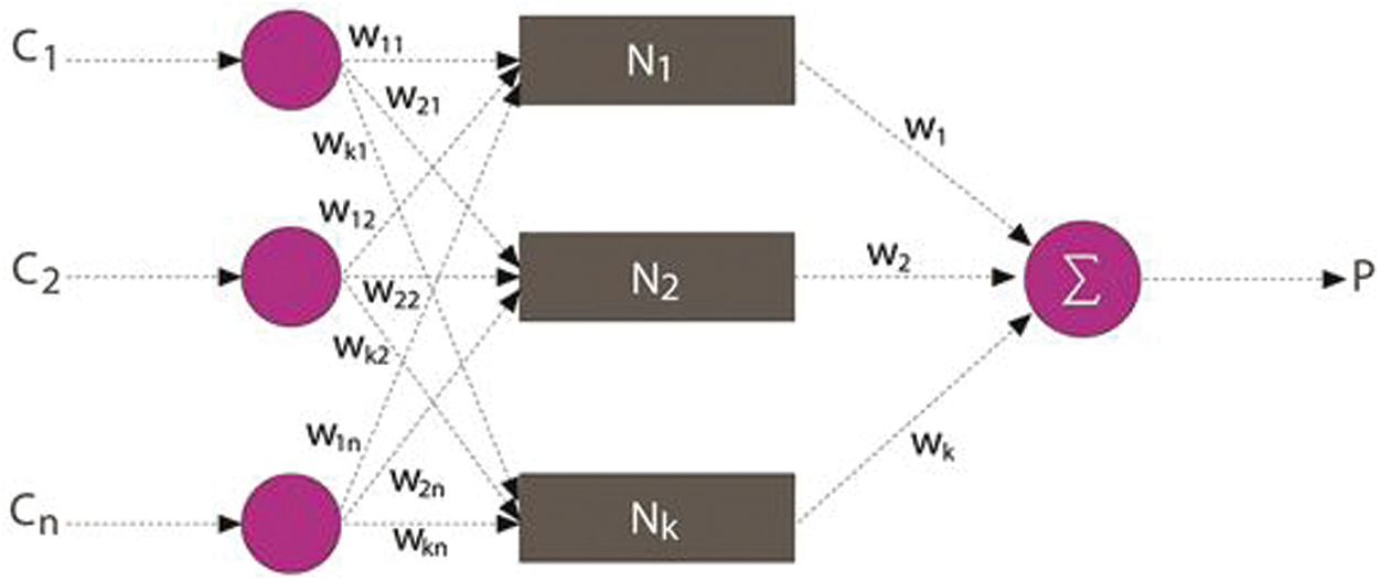
Figure 3: Architecture of MLP [23]
There are some factors that affect the prediction ability and precision of MLP ANN. Number of neurons and transfer function are among the most crucial parameters. In this regard, different numbers of neurons are tested in the network. Furthermore, to investigate the effect of the transfer function, three different functions including radial basis, tansig and logsig are used. These functions are presented in Fig. 4.
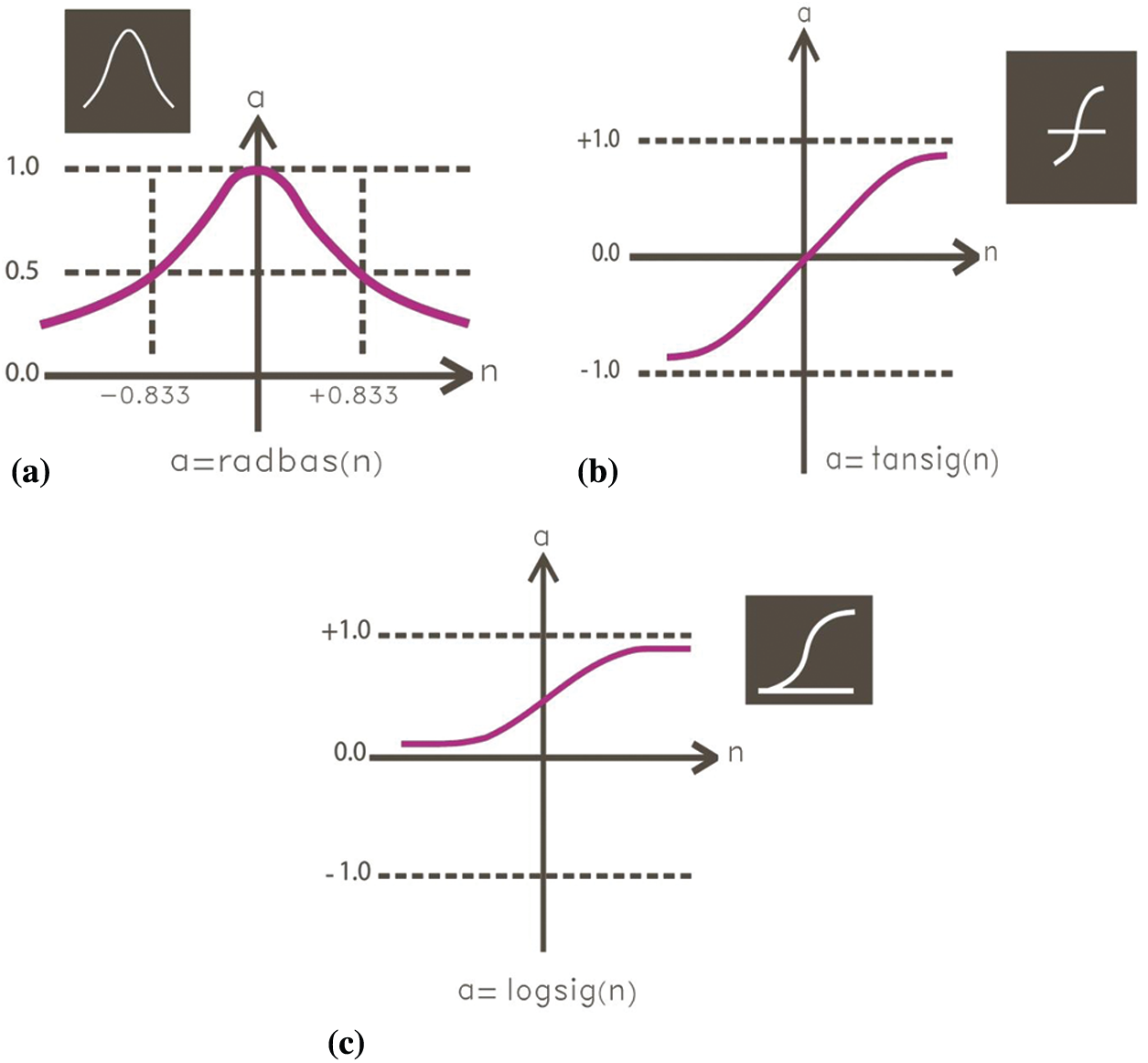
Figure 4: Schematic of (a) radial basis, (b) tansig, and (c) logsig functions
In order to train the networks, the consumptions of coal, oil, natural gas, hydroelectricity, other renewable energies and GDP are applied as inputs. Moreover, single hidden layer is utilized in the network. The energy source consumptions are extracted from Ref. [21] and GDP of the countries are gathered from Ref [25]. It should be mentioned that available data between 1990 and 2019 are considered in this study. The data were randomly divided into three subgroups for training (70%), validation (15%) and test (15%). For comparing the results, three criteria including R-squared, mean squared error (MSE) and average absolute relative deviation (AARD) are considered which can be determined as follows [26]:
where n is the number of datasets, and
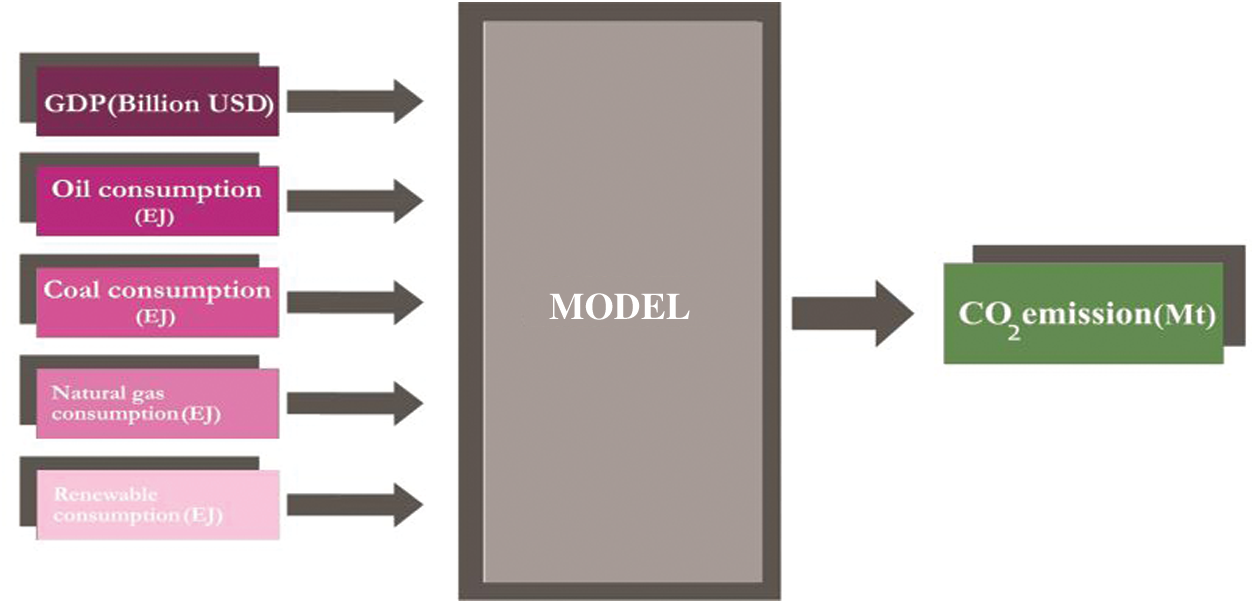
Figure 5: Schematic of the model with its inputs
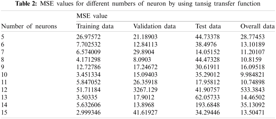
In this study, three different transfer functions with various numbers of neurons, ranging from 5 to 15 are tested to reach an accurate predictive model. In order to assess the model, MSE values are compared and the lowest case is selected as the most accurate one. In Tab. 2, the MSE values of the trained network for case of using tansig transfer function are represented. As shown in this table, in case of using 10 neurons, the lowest value of the network is obtained which is around 9.98.
As indicated in the previous section, the data are divided into three subgroups. In Figs. 6–9, the predicted values vs. actual ones are compared for all of the subgroups in addition to the overall data. The R-squared value of the trained network for the overall data as shown in Fig. 9 is 0.9996, indicating remarkable accuracy of the prediction.
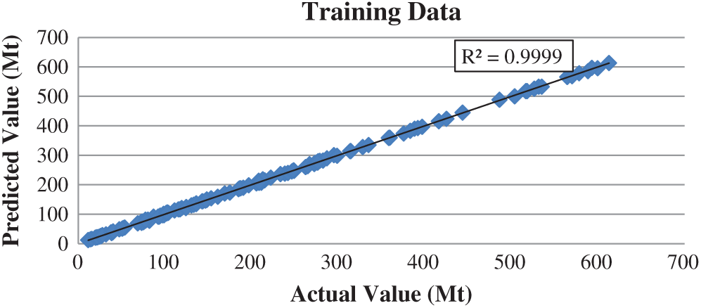
Figure 6: Predicted data vs. actual value for training data with tansig transfer function
In addition to tansig, logsig transfer function is applied in the network. In this condition, as shown in Tab. 3, the highest accuracy is obtained by utilizing 13 neurons in the hidden layer of the network. In this condition, MSE value of the model equals to 6.42 which is lower in comparison with the network using tansig transfer function. The lower value of the MSE indicates higher accuracy of the network with logsig transfer function.
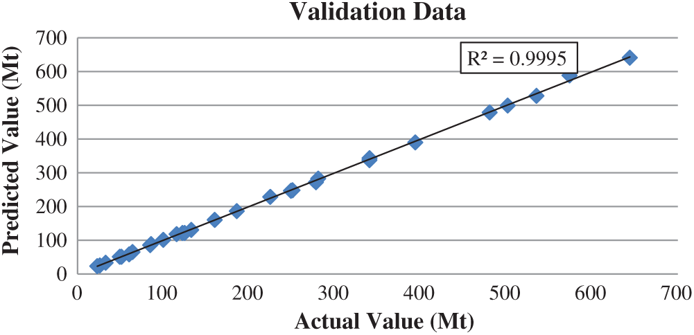
Figure 7: Predicted data vs. actual value for validation data with tansig transfer function
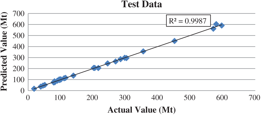
Figure 8: Predicted data vs. actual value for test data with tansig transfer function
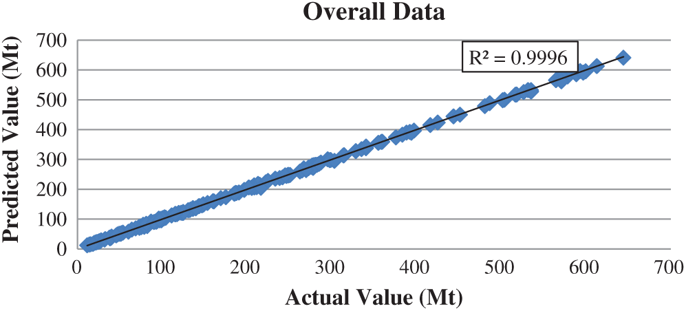
Figure 9: Predicted data vs. actual value for overall data with tansig transfer function
In Figs. 10–13, the actual values are compared with the predicted ones obtained by applying the network using logsig transfer function with 13 neurons in the hidden layer. In this condition, the R-squared of the model is 0.9998 which is higher than the corresponding value in case of using tansig function in the network.
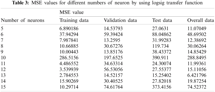
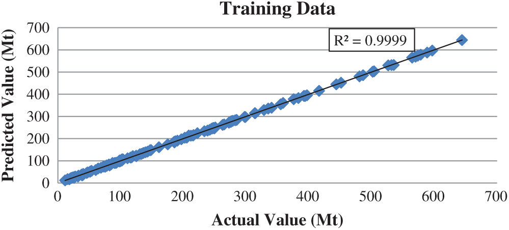
Figure 10: Predicted data vs. actual value for training data with logsig transfer function
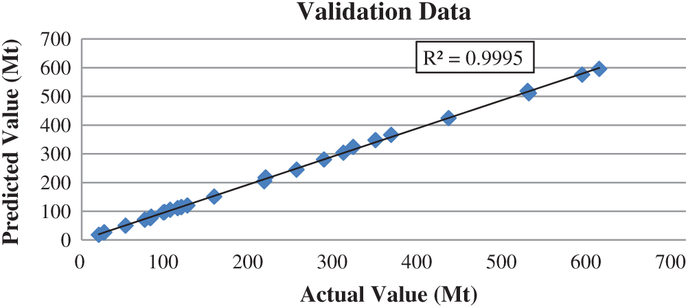
Figure 11: Predicted data vs. actual value for validation data with logsig transfer function
Finally, radial basis function is tested as transfer function in the architecture of the network. In this case, similar numbers of neuron are used to find an accurate model. As represented in Tab. 4, the minimum value of obtained MSE value is around 8.48, which indicates its higher accuracy compared to that in the network with tansig transfer function whereas its accuracy is lower than the network with logsig function. For this network, the minimum value of MSE is obtained when 8 neurons are used in the network.
In Figs. 14–17, the actual and predicted values of carbon dioxide emission for the case studies are compared for the three subgroups listed earlier. As shown in these figures, the R-squared is 0.9997, which is higher than the corresponding value of the network with tansig function while it is lower than that in the model with logsig function. Ultimately, AARD of the designed networks in optimum condition are determined to compare them by using another criterion. As shown in Fig. 18, employing logsig leads to the minimum value of AARD, around 1.67%, while utilizing radbas leads to the maximum value of AARD which is around 2.06%. In comparison with another study conducted on Middle Eastern countries, the proposed model has higher accuracy in term of AARD. Moreover, in addition to considering more case studies, more recent data, till 2019, are considered in the current study. All of these facts denote that the present model is more applicable and reliable for CO2 emission prediction of the considered countries.
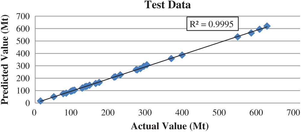
Figure 12: Predicted data vs. actual value for test data with logsig transfer function
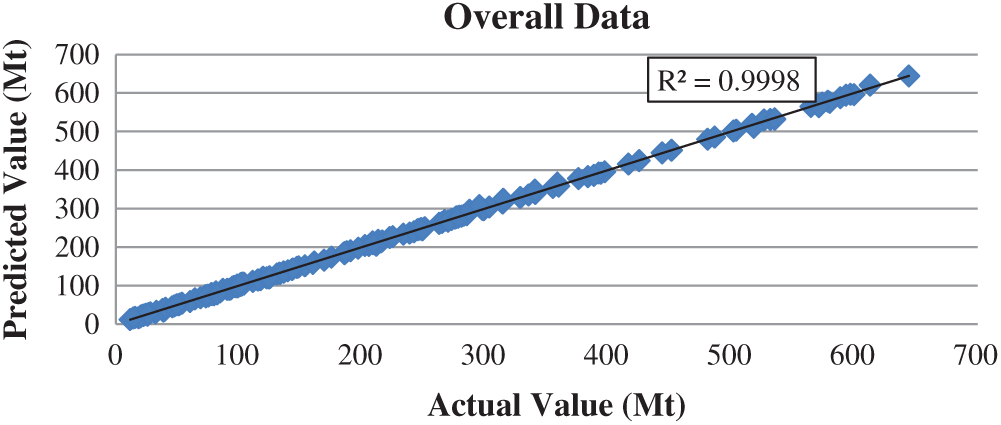
Figure 13: Predicted data vs. actual value for overall data with logsig transfer function
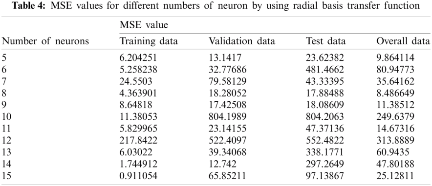
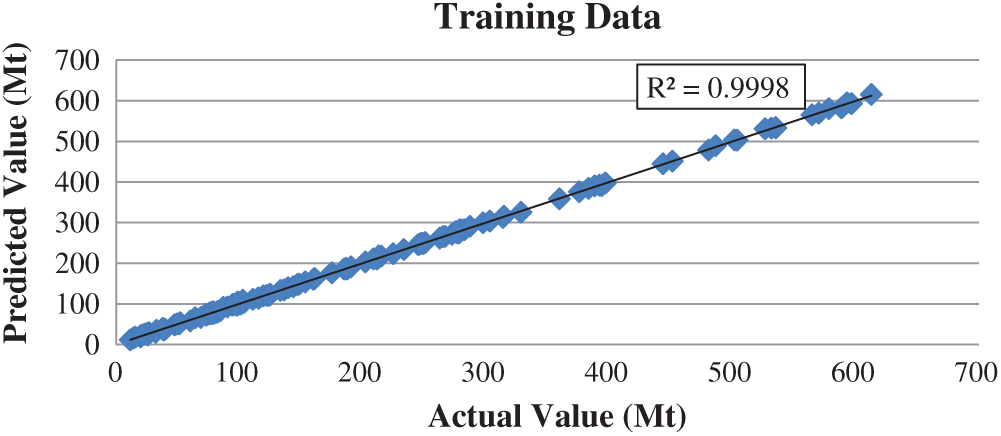
Figure 14: Predicted data vs. actual value for training data with radial basis transfer function
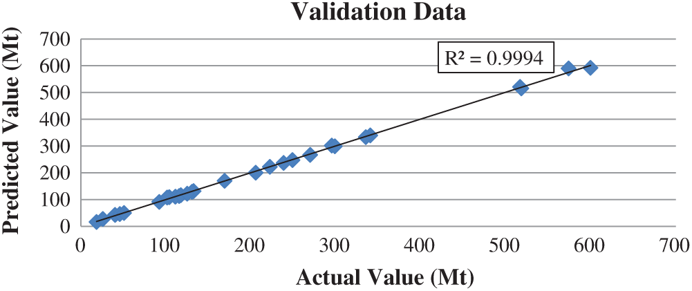
Figure 15: Predicted data vs. actual value for validation data with radial basis transfer function
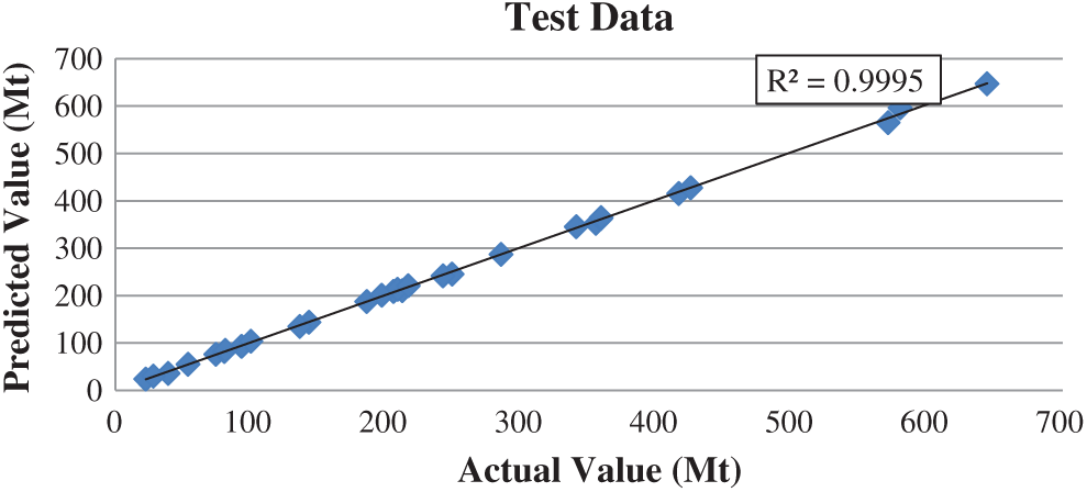
Figure 16: Predicted data vs. actual value for test data with radial basis transfer function
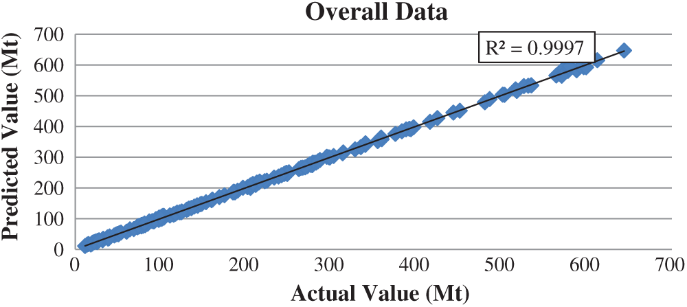
Figure 17: Predicted data vs. actual value for overall data with radial basis transfer function
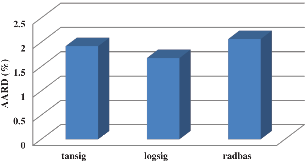
Figure 18: AARD of the proposed networks with different transfer functions
In this study, carbon dioxide emission of seven Middle Eastern countries including Iran, Turkey, Kuwait, United Arab Emirates, Saudi Arabia and Qatar were modeled by using MLP neural network with various numbers of neurons in hidden layer and different transfer functions including tansig, logsig and radial basis. Consumptions of different energy sources in addition to GDP of the mentioned countries were applied as the inputs of the models. According to the obtained results, using logsig function in the hidden layer and utilizing 13 neurons in the hidden layer led to the most accurate prediction with MSE value of 6.42 while R-squared of this model is 0.9998. In term of accuracy, this model was followed by the network with radial basis function. The R-squared and MSE of the model with radial basis function and logsig were 0.9997 and 8.48, and 0.996 and 9.98, respectively. Moreover, comparison of this model with the proposed one in a similar study, considering five countries in the same region, reveals higher accuracy in term of MSE.
Acknowledgement: The authors would like to thank A. Alhuyi Nazari for his help in editing the manuscript.
Funding Statement: This work was supported by College of Engineering and Technology, the American University of the Middle East, Kuwait. Homepage: https://www.aum.edu.kw.
Conflicts of Interest: The authors declare that they have no conflicts of interest to report regarding the present study.
1. Y. Chen, L. He, Y. Guan, H. Lu and J. Li, “Life cycle assessment of greenhouse gas emissions and water-energy optimization for shale gas supply chain planning based on multi-level approach: Case study in barnett, marcellus, fayetteville, and haynesville shales,” Energy Conversion and Management, vol. 134, no. 3, pp. 382–398, 2017. [Google Scholar]
2. H. Lu, Y. Guan, L. He, H. Adhikari, P. Pellikka, J. Heiskanen et al., “Patch aggregation trends of the global climate landscape under future global warming scenario,” International Journal of Climatology, vol. 40, no. 5, pp. 2674–2685, 2020. [Google Scholar]
3. The effects of climate change. USA: NASA, 2021. [Online]. Available: https://climate.nasa.gov/effects/. [Google Scholar]
4. L. He, Y. Chen and J. Li, “A three-level framework for balancing the tradeoffs among the energy, water, and air emission implications within the life-cycle shale gas supply chains,” Resources, Conservation and Recycling, vol. 133, no. 11, pp. 206–228, 2018. [Google Scholar]
5. Y. Chen, L. He, J. Li and S. Zhang, “Multi-criteria design of shale-gas-water supply chains and production systems towards optimal life cycle economics and greenhouse gas emissions under uncertainty,” Computers and Chemical Engineering, vol. 109, no. 4, pp. 216–235, 2018. [Google Scholar]
6. X. Han, N. Chen, J. Yan, J. Liu, M. Liu et al., “Thermodynamic analysis and life cycle assessment of supercritical pulverized coal-fired power plant integrated with No.0 feedwater pre-heater under partial loads,” Journal of Cleaner Production, vol. 233, no. 11, pp. 1106–1122, 2019. [Google Scholar]
7. A. Maleki, A. Haghighi, M. E. Assad, I. Mahariq and M. A. Nazari, “A review on the approaches employed for cooling PV cells,” Solar Energy, vol. 209, no. 10, pp. 170–185, 2020. [Google Scholar]
8. A. Haghighi, M. R. Pakatchian, M. E. H. Assad, V. N. Duy and M. Alhuyi Nazari, “A review on geothermal organic rankine cycles: Modeling and optimization,” Journal of Thermal Analysis and Calorimetry, vol. 10, no. 2, pp. 1–16, 2020. [Google Scholar]
9. Y. S. Bhagavatula, M. T. Bhagavatula and K. S. Dhathathreyan, “Application of artificial neural network in performance prediction of PEM fuel cell,” International Journal of Energy Research, vol. 36, no. 13, pp. 1215–1225, 2012. [Google Scholar]
10. Y. Wang, M. L. Kamari, S. Haghighat and P. T. T. Ngo, “Electrical and thermal analyses of solar PV module by considering realistic working conditions,” Journal of Thermal Analysis and Calorimetry, vol. 2, no. 1, pp. 1–10, 2020. [Google Scholar]
11. M. H. Ahmadi, M. A. Ahmadi, M. A. Nazari, O. Mahian and R. Ghasempour, “A proposed model to predict thermal conductivity ratio of Al2O3/EG nanofluid by applying least squares support vector machine (LSSVM) and genetic algorithm as a connectionist approach,” Journal of Thermal Analysis and Calorimetry, vol. 135, no. 1, pp. 271–281, 2019. [Google Scholar]
12. M. H. Esfe, S. Esfandeh, M. Afrand, M. Rejvani and S. H. Rostamian, “Experimental evaluation, new correlation proposing and ANN modeling of thermal properties of EG based hybrid nanofluid containing ZnO-dWCNT nanoparticles for internal combustion engines applications,” Applied Thermal Engineering, vol. 133, no. 2, pp. 452–463, 2018. [Google Scholar]
13. F. Mohamadian, L. Eftekhar and Y. H. Bardineh, “Applying GMDH artificial neural network to predict dynamic viscosity of an antimicrobial nanofluid,” Nanomedicine Journal, vol. 5, no. 4, pp. 217–221, 2018. [Google Scholar]
14. M. Ghalandari, H. Forootan Fard, A. K. Birjandi and I. Mahariq, “Energy-related carbon dioxide emission forecasting of four european countries by employing data-driven methods,” Journal of Thermal Analysis and Calorimetry, vol. 22, no. 5, pp. 1–10, 2020. [Google Scholar]
15. M. H. Rezaei, M. Sadeghzadeh, M. A. Nazari, M. H. Ahmadi and F. R. Astaraei, “Applying GMDH artificial neural network in modeling CO2 emissions in four nordic countries,” International Journal of Low-Carbon Technologies, vol. 13, no. 3, pp. 266–271, 2018. [Google Scholar]
16. M. H. Ahmadi, M. D. Madvar, M. Sadeghzadeh, M. H. Rezaei, M. Herrera et al., “Current status investigation and predicting carbon dioxide emission in latin American countries by connectionist models,” Energies, vol. 12, no. 10, pp. 1916–1928, 2019. [Google Scholar]
17. M. H. Ahmadi, M. D. Madvar, M. Sadeghzadeh, M. H. Rezaei, M. Herrera et al., “Current status investigation and predicting carbon dioxide emission in latin American countries by connectionist models,” Energies, vol. 12, no. 10, pp. 1916–1929, 2019. [Google Scholar]
18. M. Ghazvini, M. D. Madvar, M. A. Ahmadi, M. H. Rezaei, E. H. Assad et al., “Technological assessment and modeling of energy-related CO2 emissions for the G8 countries by using hybrid IWO algorithm based on SVM,” Energy Science & Engineering, vol. 8, no. 4, pp. 1285–1308, 2020. [Google Scholar]
19. M. H. Ahmadi, H. Jashnani, K. W. Chau, R. Kumar and M. A. Rosen, “Carbon dioxide emissions prediction of five Middle Eastern countries using artificial neural networks,” Energy Sources, Part A: Recovery, Utilization and Environmental Effects, vol. 23, no. 7, pp. 1–15, 2019. [Google Scholar]
20. Population Total. Worldwide: The Worlf Bank of Data, 2021. [Online]. Available: https://data.worldbank.org. [Google Scholar]
21. BP Statistical Review of World Energy. WorlWide: bP oil Company, 2020. [Online]. Available: https://www.bp.com/en/global/corporate/energy-economics/statistical-review-of-world-energy.html. [Google Scholar]
22. Reports about Energy. Worldwide: International Energey Agency (IEA2021. [Online]. Available: https://www.iea.org/countries. [Google Scholar]
23. M. Ramezanizadeh, M. H. Ahmadi, M. A. Nazari, M. Sadeghzadeh and L. Chen, “A review on the utilized machine learning approaches for modeling the dynamic viscosity of nanofluids,” Renewable and Sustainable Energy Reviews, vol. 114, no. 1, pp. 109345–109359, 2019. [Google Scholar]
24. M. Ramezanizadeh, M. A. Nazari, M. H. Ahmadi, G. Lorenzini and I. Pop, “A review on the applications of intelligence methods in predicting thermal conductivity of nanofluids,” Journal of Thermal Analysis and Calorimetry, vol. 19, no. 3, pp. 1–17, 2019. [Google Scholar]
25. Gross Domesitic Product by Country GDP (current US$). Worldwide: The Worlf Bank of Data, 2021. [Online]. Available: https://data.worldbank.org/indicator. [Google Scholar]
26. A. Maleki, A. Haghighi, M. I. Shahrestani and Z. Abdelmalek, “Applying different types of artificial neural network for modeling thermal conductivity of nanofluids containing silica particles,” Journal of Thermal Analysis and Calorimetry, vol. 8, no. 3, pp. 1–16, 2020. [Google Scholar]
 | This work is licensed under a Creative Commons Attribution 4.0 International License, which permits unrestricted use, distribution, and reproduction in any medium, provided the original work is properly cited. |