DOI:10.32604/cmc.2021.019061
| Computers, Materials & Continua DOI:10.32604/cmc.2021.019061 | |
| Article |
Entropy Bayesian Analysis for the Generalized Inverse Exponential Distribution Based on URRSS
1Faculty of Science, Department of Mathematics, Al al-Bayt University, Mafraq, 25113, Jordan
2Faculty of Graduate Studies for Statistical Research, Cairo University, Giza, 12613, Egypt
3Department of Mathematics, College of Science and Human Studies at Hotat Sudair, Majmaah University, Majmaah, 11952, Saudia Arabia
*Corresponding Author: Ayed R. A. Al-Anzi. Email: a.alanzi@mu.edu.sa
Received: 31 March 2021; Accepted: 03 May 2021
Abstract: This paper deals with the Bayesian estimation of Shannon entropy for the generalized inverse exponential distribution. Assuming that the observed samples are taken from the upper record ranked set sampling (URRSS) and upper record values (URV) schemes. Formulas of Bayesian estimators are derived depending on a gamma prior distribution considering the squared error, linear exponential and precautionary loss functions, in addition, we obtain Bayesian credible intervals. The random-walk Metropolis-Hastings algorithm is handled to generate Markov chain Monte Carlo samples from the posterior distribution. Then, the behavior of the estimates is examined at various record values. The output of the study shows that the entropy Bayesian estimates under URRSS are more convenient than the other estimates under URV in the majority of the situations. Also, the entropy Bayesian estimates perform well as the number of records increases. The obtained results validate the usefulness and efficiency of the URV method. Real data is analyzed for more clarifying purposes which validate the theoretical results.
Keywords: Shannon entropy; generalized inverse exponential distribution; Bayesian estimators; loss function; ranked set sampling; markov chain
Record values are crucial in many areas of real life applications comprising data relating to weather, sports, economics and life testing studies. Reference [1] constructed the theory of record values as a model for successive extremes in a sequence of independently and identically distributed (iid) random variables. Reference [2] mentioned that an observation is called upper (lower) record value if its value more (less than) that all of the preceding observations. Let xi,
Let
where
Another record sampling scheme, known as upper record ranked set sampling, has been provided by [3]. This scheme is valuable in some situations when the used observations are the last record data such as athletic, weather and Olympic data. The URRSS can be described as follows:
Consider n independent sequences of continuous random variables, the
where
For information about ranked set sampling, see [4] for imputation of the missing observations using RSS and [5] for mean estimation based on modified robust extreme ranked set sampling. References [6–8] for partial, mixed and varied RSS methods, respectively. Reference [9] proposed a new RSS technique for mean and variance estimation, as well as [10] investigated the estimation of a symmetric distribution function in multistage ranked set sampling.
Some researchers have considered inference about different distributions based on records. For instance, Bayesian estimators and predictions for some life distributions from record values are discussed by [11]. Stress-strength reliability estimator of exponentiated inverted Weibull distribution values has been discussed by [12] based on lower record. Reference [13] considered Bayesian and non-Bayesian estimators from power Lomax distribution using URV. Estimation of the two-parameter bathtub-shaped distribution is discussed by [14] from record data. Bayesian estimators of the generalized inverse exponential (GIE) distribution are discussed by [15] via URV. Stress strength reliability estimator for independent GIE distributions using URRSS is handled by [16]. Reference [17] discussed estimation and prediction for Nadarajah-Haghighi distribution based on record. Statistical inference for the power Lindley model is studied by [18] from record values and inter-record times. Reference [19] handled reliability estimator for Weibull distribution for multicomponent system based on URV.
Reference [20] introduced the concept of entropy as a measure of information, which provides a quantitative measure of the uncertainty. It is also considered as a measure of randomness of a probabilistic system. Let X be a non-negative random variable with cumulative distribution function F(x) and probability density function f(x). The Shannon entropy, denoted by SH(X), of the random variable is defined by
It is seen that a very sharply peaked distribution has very low entropy, whereas if the probability is spread out, the entropy is much higher. In this sense, SH(X) is a measure of uncertainty associated with f(x). Entropy estimation for some life distributions has been discussed by many authors. For example, [21] obtained an entropy estimator using URV from the generalized half-logistic distribution. References [22,23] suggested some entropy estimators based on RSS and double RSS methods, respectively. Reference [24] investigated entropy estimation and goodness-of-fit tests for the Laplace and inverse Gaussian distributions based on pair RSS. Reference [25] discussed the entropy Bayesian estimators of Weibull distribution based on generalized progressive hybrid censoring scheme. Reference [26] proposed new measures of entropy and [27] discussed the entropy maximum likelihood and Bayesian estimators of inverse Weibull distribution under generalized progressive hybrid censoring scheme. Reference [28] provided an exact expression for entropy information contained in both types of progressively hybrid censored data and applied it in exponential distribution. Reference [29] discussed the estimation of entropy for generalized exponential distribution via record values. Reference [30] discussed entropy estimators of a continuous random variable using RSS. Reference [31] obtained the maximum likelihood estimator of Shannon entropy for inverse Weibull distribution under multiple censored data and [32] proposed entropy Bayesian estimators of Lomax distribution using record data, and [33] considered extropy properties of RSS.
To our knowledge, in the literature, there are no studies that had been performed about entropy estimation in view of URRSS. So, our interest in this study is estimating the Shannon entropy of the GIE distribution using Bayesian approach from URRSS and URV. The Shannon entropy Bayesian estimator is considered using gamma priors. The Bayesian estimator of entropy is induced related to symmetric and asymmetric loss functions. The proposed loss functions are squared error loss function (SELF), linear exponential loss function (LINEX) and precautionary loss function (PRLF). Bayesian entropy estimators under symmetric and asymmetric loss functions have complicated expressions, so we implemented the Markov Chain Monte Carlo (MCMC) technique.
The following sections are organized as follows. Formula of Shannon entropy for GIE distribution is provided in Section 2. Entropy Bayesian estimator is derived using URRSS from symmetric and asymmetric loss functions in Section 3. Based on URV, entropy Bayesian estimator for GIE distribution is discussed using the proposed loss functions in Section 4. Simulation issue and application to real data are given in Sections 5 and 6, respectively. The paper ends with some concluding remarks in Section 7.
2 Expression of Shannon Entropy
The two-parameter GIE distribution is provided by [34] which has many applications in various areas such as, accelerated life testing, queues, horse racing, sea currents and wind speeds. The PDF of the GIE model with the shape parameter
The CDF of the GIE distribution is given by
Let X be a random variable follows a GIE distribution with PDF given in (4), hence the Shannon entropy of X is obtained by substituting (4) in (3) as follows:
where
and
where
Also, I3 is obtained as follows
Substituting I1, I2, and I3 in (6), we obtain the Shannon entropy for GIE distribution as follows:
which is a function of the parameters
3 Entropy Bayesian Estimation Based on URRSS
In this section, Bayesian estimator of the Shannon entropy for the GIE model is discussed in view of URRSS. Firstly, the Bayesian estimators of parameters must be computed in order to get the entropy Bayesian estimator. Then, entropy Bayesian estimator is obtained using (7) according to the invariance property. The Bayesian estimator based on gamma priors is considered. Three Bayesian estimators are obtained according to SELF, LINEX and PRLF. Furthermore, the Bayesian credible intervals are constructed.
Let
Assuming that the prior of parameters
The joint posterior under the assumption that
Hence, the marginal posterior distributions of
where
Therefore, the Bayesian estimators of
The Bayesian estimators of
and
where
and
The integrals (9)–(13) are very hard to be solved analytically according to their convoluted forms. Therefore, we employ the MCMC technique to approximate these integrations. The Bayesian estimates together with credible intervals width under SELF, LINEX and PRLF loss functions are implemented using Metropolis-Hastings (M-H) algorithm. Therefore, the Bayes estimate of SH(X), denoted by
Consequently, the Bayesian estimator of SH(X) under LINEX and PRLF are obtained by similar way after setting their estimators in (7). Additionally, we get the Bayesian credible interval of entropy using the same algorithm proposed by [35].
4 Entropy Bayesian Estimation Based on URV
This section provides the Bayesian estimators of
Assuming that the prior of
Consequently, expressions for the marginal posterior distributions of
where
Hence, Bayesian estimators of
Also, under LINEX, the Bayesian estimators of
Furthermore, considering PRLF, the Bayesian estimators of
Again, the MCMC procedure is provided to approximate the integrals (14)–(16) based on M-H algorithm to compute the estimates and credible interval width considering symmetric and asymmetric loss functions.
Regarding to Eq. (7), the Bayesian estimator of SH(x), denoted by
By similar way, the Bayesian estimator of SH(X) under LINEX and PRLF are obtained after setting their estimators in (7). Furthermore, the Bayesian credible interval is obtained as mentioned in the Section 3.
In this section, a simulation investigation is carried out to compare the performance of the entropy estimate of the GIE distribution based on URV and URRSS. The relative absolute bias (RAB), estimated risk (ER) and width (WD) of credible intervals for the Shannon entropy based on URV and URRSS for GIE distribution are used to evaluate the behaviour of the Bayesian estimates. In the simulation setup, the number of records are selected as
The M-H algorithm procedure is described as follows:
Let g(.) be the density of subject distribution.
Initialize a starting value
for
set
generate u from U(0, 1)
generate y from g(.)
if
set
else
set
end if
end for
Tabs. 1–3 summarize the Bayes estimates and their measures (RAB, ER and WD) based on URV and URRSS. From the numerical outcomes given in Tabs. 1–3 and Figs. 1–6, we can conclude the following:
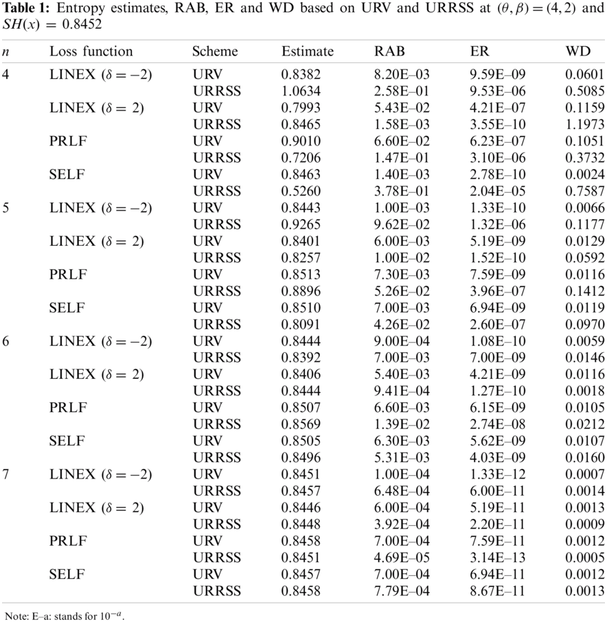
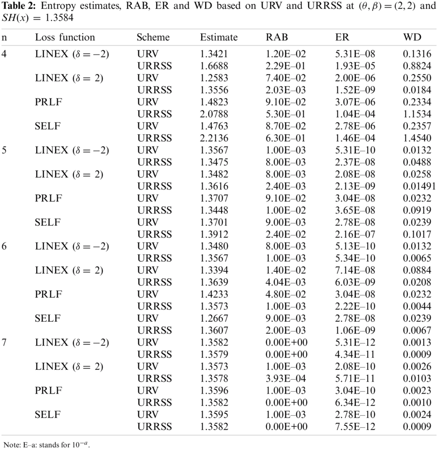
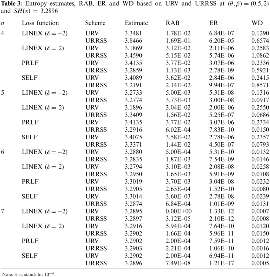
• The ER of entropy estimates under SELF and LINEX based on URRSS is smaller than that of the corresponding under URV at n = 6 for all values of
• The ER of entropy estimates under LINEX (
• The ER of entropy estimates based on URSS is smaller than the corresponding under URV at n = 5, and
• The ER of entropy estimates based on URRSS is smaller than the corresponding under URV at n = 7,
• The WD of entropy estimates based on URV is smaller than the corresponding under URRSS at n = 4 under PRLF for all values of
• In general, as n increases, the ER, RAB and WD of estimate decrease for both record schemes.
• As the true value SH(x) increases, the ER increases in most of the situations.
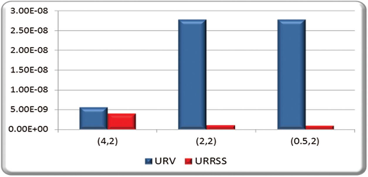
Figure 1: ER of entropy estimate based on URV and URRSS at SELF and
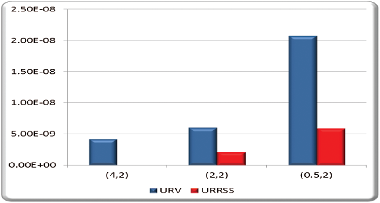
Figure 2: ER of entropy estimate based on URV and URRSS at
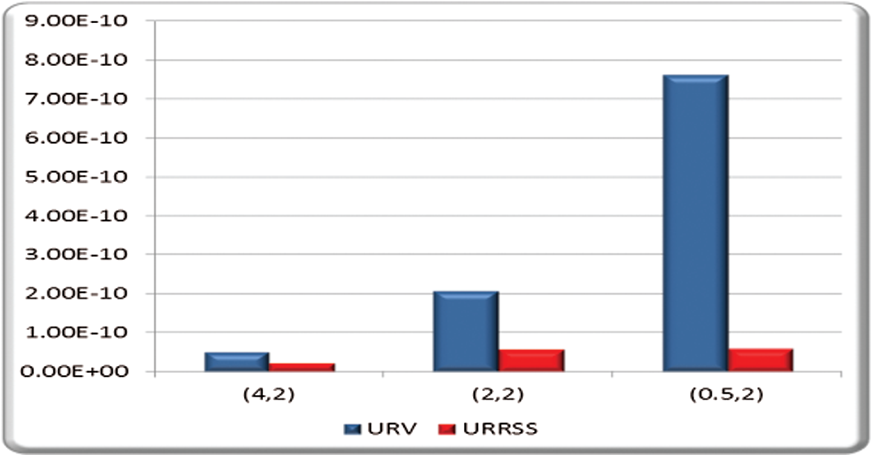
Figure 3: ER of entropy estimate based on URV and URRSS at
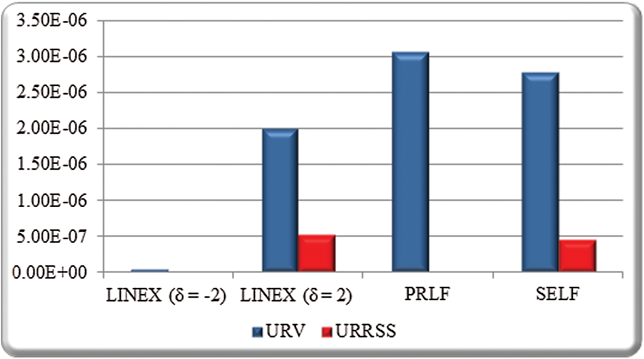
Figure 4: ER of entropy estimate based on URV and URRSS at
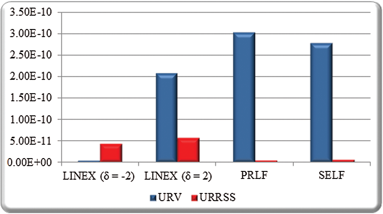
Figure 5: ER of entropy estimate based on URV and URRSS at
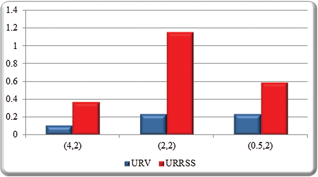
Figure 6: WD of entropy estimate based on URV and URRSS at
In this section, a real data set is analysed for illustrative purposes. The suggested data represent the lifetimes of steel specimens tested at different stress levels (for more details see [36]. Some preliminary data analysis is performed. The Kolmogorov-Smirnov (K-S) test is used for the data set to the fitted model. It is observed that the K-S distance are 0.083 with the corresponding P-value 0.917. It indicates that the GIE model provides reasonable fit to this data set. Also, the estimated PDF, CDF and PP plots for data are represented in Fig. 7. From these figures it can be concluded that the GIE distribution is an adequate model to fit these data.
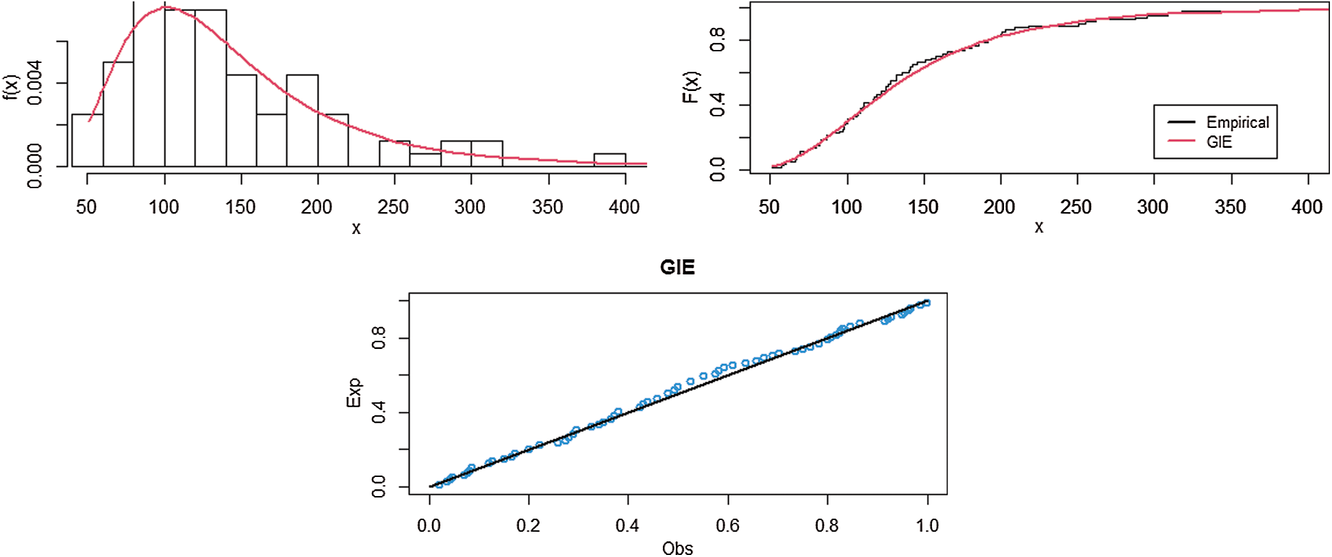
Figure 7: Estimated PDF, CDF and PP plots of the GIE distribution for lifetimes of steel specimens data
The extracted records from a part of this data are presented as
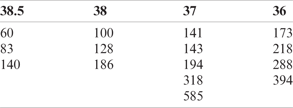
Based on the above record data, it can be shown that URRSS of size n = 4 is
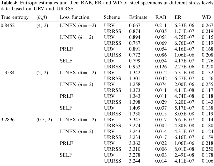
From Tab. 4, we can conclude that ER of entropy estimates under URRSS gets the smallest values compared to the corresponding under URV in case of PRLF and LINEX
This paper provides Bayesian estimation of the Shannon entropy for the generalized inverse exponential distribution using URRSS and URV shemes. The entropy Bayesian estimators are considered using gamma prior functions for symmetric (SELF) and asymmetric (LINEX and PRLF) loss functions. In order to obtain the Bayesian estimators, we employed Markov Chain Monte Carlo method based on Metropolis-Hastings algorithm. The performance of the entropy estimates for the GIE distribution is investigated in terms of their relative absolute bias, estimated risk and the width of credible intervals. From simulation results, it turns out that, the entropy Bayesian estimator approaches the true value as the number of record increases. Generally, the entropy and ERs are directly proportional, that is; if the real value of entropy increases, the ERs increase. The WD of Bayes credible intervals for estimated values of entropy URRSS is smaller than the corresponding estimated values based on URV for all loss functions for most values of record values in the majority of the cases. A data real example has been considered to illustrate the applicability of the proposed methodology for the considered record schemes.
Acknowledgement: The authors are grateful to the Editor and anonymous reviewers for their valuable comments and suggestions.
Funding Statement: A. R. A. Alanzi would like to thank the Deanship of Scientific Research at Majmaah University for financial support and encouragement.
Conflicts of Interest: The authors declare that they have no conflicts of interest to report regarding the present study.
1. K. Chandler, “The distribution and frequency of record values,” Journal of the Royal Statistical Society: Series B (Methodological), vol. 14, no. 2, pp. 220–228, 1952. [Google Scholar]
2. H. Arnold, B. Balakrishnan and N. Nagaraja, Records, New York: John Wiley & Sons, 1998. [Google Scholar]
3. M. Salehi and J. Ahmadi, “Record ranked set sampling scheme,” Metron, vol. 72, no. 3, pp. 351–365, 2014. [Google Scholar]
4. C. N. Bouza and A. I. Al-Omari, “Ranked set estimation with imputation of the missing observations: The median estimator,” Revista Investigacion Operacional, vol. 32, no. 1, pp. 30–37, 2011. [Google Scholar]
5. A. I. Al-Omari, “Estimation of mean based on modified robust extreme ranked set sampling,” Journal of Statistical Computation and Simulation, vol. 81, no. 8, pp. 1055–1066, 2011. [Google Scholar]
6. A. Haq, J. Brown, E. Moltchanova and A. I. Al-Omari, “Partial ranked set sampling design,” Environmetrics, vol. 24, no. 3, pp. 201–207, 2013. [Google Scholar]
7. A. Haq, J. Brown, E. Moltchanova and A. I. Al-Omari, “Mixed ranked set sampling design,” Journal of Applied Statistics, vol. 41, no. 10, pp. 2141–2156, 2014. [Google Scholar]
8. A. Haq, J. Brown, E. Moltchanova and A. I. Al-Omari, “Varied L ranked set sampling scheme,” Journal of Statistical Theory and Practice, vol. 9, no. 4, pp. 741–767, 2015. [Google Scholar]
9. E. Zamanzade and A. I. Al-Omari, “New ranked set sampling for estimating the population mean and variance,” Hacettepe Journal of Mathematics and Statistics, vol. 45, no. 6, pp. 1891–1905, 2016. [Google Scholar]
10. M. Mahdizadeh and E. Zamanzade, “Estimation of a symmetric distribution function in multistage ranked set sampling,” Statistical Papers, vol. 61, no. 2, pp. 851–867, 2020. [Google Scholar]
11. J. Ahmadi and M. Doostparast, “Bayesian estimation and prediction for some life distributions based on record values,” Statistical Papers, vol. 47, no. 3, pp. 373–392, 2006. [Google Scholar]
12. A. S. Hassan, H. Z. Muhammed and M. S. Saad, “Estimation of stress-strength reliability for exponentiated inverted weibull distribution based on lower record values,” Journal of Advances in Mathematics and Computer Science, vol. 11, no. 2, pp. 1–14, 2015. [Google Scholar]
13. E. A. Amin, “On record values of the power lomax distribution,” Advances and Applications in Statistics, vol. 50, no. 6, pp. 497–515, 2017. [Google Scholar]
14. M. Z. Raqab, O. M. Bdair and F. M. Al-Aboud, “Inference for the two-parameter bathtub-shaped distribution based on record data,” Metrika, vol. 81, no. 3, pp. 229–253, 2018. [Google Scholar]
15. A. S. Hassan, M. Abd-Allah and H. F. Nagy, “Bayesian analysis of record statistics based on generalized inverted exponential model,” International Journal on Advanced Science, Engineering and Information Technology, vol. 8, no. 2, pp. 323–335, 2018a. [Google Scholar]
16. A. S. Hassan, A. Marwa and H. F. Nagy, “Estimation of P (Y > X) using record values from the generalized inverted exponential distribution,” Pakistan Journal of Statistics and Operation Research, vol. 14, no. 3, pp. 645–660, 2018b. [Google Scholar]
17. M. A. Selim, “Estimation and prediction for nadarajah-haghighi distribution based on record values,” Pakistan Journal of Statististics, vol. 34, no. 1, pp. 77–90, 2018. [Google Scholar]
18. A. Pak and S. Dey, “Statistical inference for the power lindley model based on record values and inter-record times,” Journal of Computational and Applied Mathematics, vol. 347, pp. 156–172, 2019. [Google Scholar]
19. A. S. Hassan, H. F. Nagy, H. Z. Muhammed and M. S. Saad, “Estimation of multicomponent stress-strength reliability following weibull distribution based on upper record values,” Journal of Taibah University for Science, vol. 14, no. 1, pp. 244–253, 2020. [Google Scholar]
20. C. E. Shannon, “A mathematical theory of communication,” The Bell System Technical Journal, vol. 27, no. 3, pp. 379–423, 1948. [Google Scholar]
21. J.-I. Seo, H.-J. Lee and S.-B. Kang, “Estimation for generalized half logistic distribution based on records,” Journal of the Korean Data and Information Science Society, vol. 23, no. 6, pp. 1249–1257, 2012. [Google Scholar]
22. A. I. Al-Omari, “Estimation of entropy using random sampling,” Journal of Computational and Applied Mathematics, vol. 261, pp. 95–102, 2014. [Google Scholar]
23. A. I. Al-Omari, “New entropy estimators with smaller root mean squared error,” Journal of Modern Applied Statistical Methods, vol. 14, no. 2, pp. 88–109, 2015. [Google Scholar]
24. A. I. Al-Omari and A. Haq, “Entropy estimation and goodness-of-fit tests for the inverse Gaussian and laplace distributions using paired ranked set sampling,” Journal of Statistical Computation and Simulation, vol. 86, no. 11, pp. 2262–2272, 2016. [Google Scholar]
25. Y. Cho, H. Sun and K. Lee, “Estimating the entropy of a weibull distribution under generalized progressive hybrid censoring,” Entropy, vol. 17, no. 1, pp. 102–122, 2015. [Google Scholar]
26. A. I. Al-Omari, “A new measure of entropy of continuous random variable,” Journal of Statistical Theory and Practice, vol. 10, no. 4, pp. 721–735, 2016. [Google Scholar]
27. K. Lee, “Estimation of entropy of the inverse weibull distribution under generalized progressive hybrid censored data,” Journal of the Korean Data & Information Science Society, vol. 28, no. 3, pp. 659–668, 2017. [Google Scholar]
28. A. Bader, “On the entropy of progressive hybrid censoring schemes,” Applied Mathematics & Information Sciences, vol. 11, no. 6, pp. 1811–1814, 2017. [Google Scholar]
29. M. Chacko and P. Asha, “Estimation of entropy for generalized exponential distribution based on record values,” Journal of the Indian Society for Probability and Statistics, vol. 19, no. 1, pp. 79–96, 2018. [Google Scholar]
30. A. I. Al-Omari and A. Haq, “Novel entropy estimators of a continuous random variable,” International Journal of Modeling, Simulation, and Scientific Computing,” vol. 10, no. 2, pp. 1950004, 2019. [Google Scholar]
31. A. S. Hassan and A. N. Zaky, “Estimation of entropy for inverse weibull distribution under multiple censored data,” Journal of Taibah University for Science, vol. 13, no. 1, pp. 331–337, 2019. [Google Scholar]
32. A. S. Hassan and A. N. Zaky, “Entropy bayesian estimation for lomax distribution based on record,” Thailand Statistician, vol. 19, no. 1, pp. 95–114, 2021. [Google Scholar]
33. M. Raqab and G. Qiu, “On extropy properties of ranked set sampling,” Statistics, vol. 53, no. 1, pp. 210–226, 2019. [Google Scholar]
34. A. Abouammoh and A. M. Alshingiti, “Reliability estimation of generalized inverted exponential distribution,” Journal of Statistical Computation and Simulation, vol. 79, no. 11, pp. 1301–1315, 2019. [Google Scholar]
35. M.-H., Chen and Q.-M. Shao, “Monte carlo estimation of Bayesian credible and HPD intervals,” Journal of Computational and Graphical Statistics, vol. 8, no. 1, pp. 69–92, 1999. [Google Scholar]
36. J. F. Lawless, Statistical Models and Methods for Lifetime Data, 2nd ed., Hoboken, New Jersey: John Wiley & Sons, Inc., 2003. [Google Scholar]
 | This work is licensed under a Creative Commons Attribution 4.0 International License, which permits unrestricted use, distribution, and reproduction in any medium, provided the original work is properly cited. |