DOI:10.32604/cmc.2021.019178
| Computers, Materials & Continua DOI:10.32604/cmc.2021.019178 | |
| Article |
Transfer Learning Model to Indicate Heart Health Status Using Phonocardiogram
1Department of Computer Science and Engineering, Thapar Institute of Engineering and Technology, Patiala, Punjab, India
2Associate Application, IT, Concentrix, Gurugram, Haryana, India
3School of Computer Software, Daegu Catholic University, Gyeongsan, Korea
4Department of Computer Engineering, Gachon University, Seongnam, 13120, Korea
5Information Security Engineering, Soonchunhyang University, Korea
6Department of Computer Engineering, University College of Engineering, Punjabi University, Patiala, Punjab, India
*Corresponding Author: Chang Choi. Email: changchoi@gachon.ac.kr
Received: 05 April 2021; Accepted: 10 May 2021
Abstract: The early diagnosis of pre-existing coronary disorders helps to control complications such as pulmonary hypertension, irregular cardiac functioning, and heart failure. Machine-based learning of heart sound is an {efficient} technology which can help minimize the workload of manual auscultation by automatically identifying irregular cardiac sounds. Phonocardiogram (PCG) and electrocardiogram (ECG) waveforms provide the much-needed information for the diagnosis of these diseases. In this work, the researchers have converted the heart sound signal into its corresponding repeating pattern-based spectrogram. PhysioNet 2016 and PASCAL 2011 have been taken as the benchmark datasets to perform experimentation. The existing models, viz. MobileNet, Xception, Visual Geometry Group (VGG16), ResNet, DenseNet, and InceptionV3 of Transfer Learning have been used for classifying the heart sound signals as normal and abnormal. For PhysioNet 2016, DenseNet has outperformed its peer models with an accuracy of 89.04 percent, whereas for PASCAL 2011, VGG has outperformed its peer approaches with an accuracy of 92.96 percent.
Keywords: PCG signals; transfer learning; repeating pattern-based spectrogram; biomedical signals; internet of things (IoT)
IoT enabled devices have opened many opportunities in the area of medical diagnosis and treatment, ensuring safety and health of patients, and empowering medical practitioners to deliver better care. The increased and sophisticated interaction with the patients is possible due to enormous, personalized data generated by these devices. The analysis of data helps the doctors to diagnose patients more efficiently. Further, remote monitoring of patients’ health enables the medical practitioners to assess situations for admission to hospital, minimizing the patient load, and hence, improves treatment outcomes and significantly reduces the healthcare costs. IoT enables proactive engagement of the patients by healthcare professionals [1]. Physicians can identify the best treatment plans and achieve the best results by having access to personalized data collected through these IoT devices [2]. Fig. 1 presents the architecture of an IoT, where each stage captures or processes data to provide an input for the next stage. Integrated values in the process bring intuitions and deliver dynamic business prospects. The steps are explained as below:
(I) Deployment of interconnected devices for data generation (e.g., sensors, actuators, monitors, detectors, camera systems, etc.).
(II) Analog to Digital conversion, aggregation of data.
(III) Pre-processing, cleaning, and storage into cloud.
(IV) Advanced analytics for actionable business insights needed for effective decision-making.
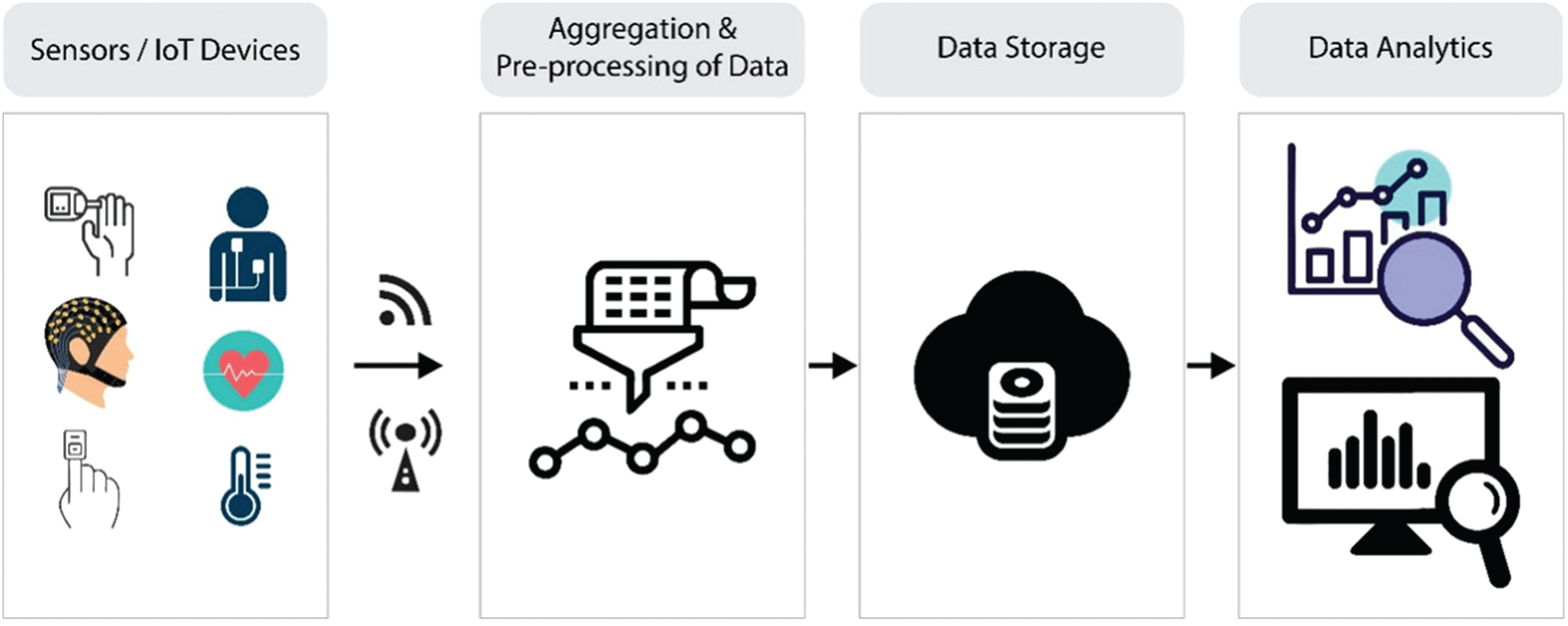
Figure 1: The architecture of an IoT-based solution
Mobility support, low latency, location, and privacy awareness are some of the advantages of a fog-based smart healthcare system [3]. Patients may receive personalized care using IoT devices such as exercise bands and other wirelessly activated devices such as cardiovascular and metabolic rate monitoring cuffs, glucometers, and so on. With IoT-connected intelligent systems, health insurers have various opportunities. Data collected by health tracking systems may be used by insurance providers for underwriting and claims processing. In the underwriting, pricing, claims management, and risk evaluation systems, IoT devices provide clarity between insurers and consumers. A detailed review undertaken by Tuli et al. [4] has shown the utility of IoT devices and artificial intelligence-based techniques for heart disease prediction system. Research community has emphasized on using ECG [5–8] w.r.t. heart health using IoT, and artificial intelligence techniques that further incorporate machine learning and deep learning approaches. Fig. 2 describes the generic architecture being followed for predicting the heart health status in real time. Where, specific sensors collect the heart-related vitals from the body and send it to the computing environment through some web-based dashboard or mobile application for further computation. Machine learning or deep learning-based models revert with the status of heart health; and the same can be seen in the mobile application or the web-based dashboard for planning the further course of action.
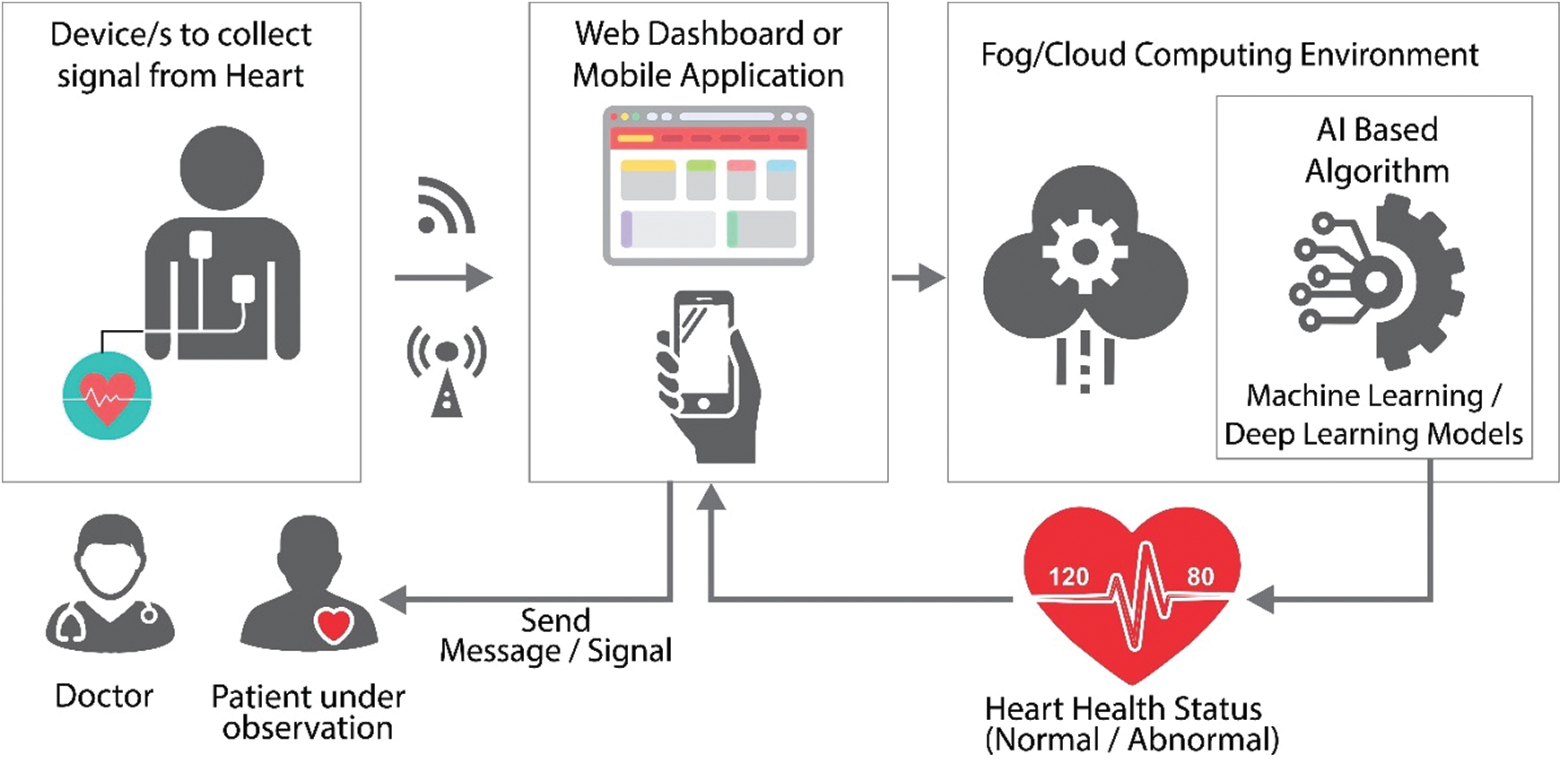
Figure 2: IoT and AI-based general architecture used for the heart healthcare
Heart Failure (HF) and its allied ailments are the major causes of death globally. The initial step for analyzing a cardiovascular system is the examination of the sound emanating from the heart. A phonocardiogram (PCG) is the graphical representation of heart sound signals [9] which allows the detection of heart murmurs and aids in visual analysis of the cardiac sound signals. The PCG signal serves as a cheaper alternative to the popular methods such as ECG, and offers almost equivalent diagnostic capabilities [10]. The procedure allows self-diagnosis and early detection of pathological heart conditions. The magnitude and frequency signals in PCG can detect additional systolic and diastolic murmurs that help in identifying heart diseases [11].
Here, in this research work, the authors have taken PCG signal instead of ECG as an input. It is believed that this is an unexplored domain in the context of given architecture in Fig. 2. Also, the input heart sound signal has been firstly converted into respective spectrogram and then classified further as normal and abnormal using the transfer learning-based model which is also an unexplored sub-domain.
1.2 Existing Approaches Based to Classify PCG Signal
Fig. 3 illustrates the generic flow for classifying a PCG signal as normal or abnormal using machine learning approaches which include three steps after data acquisition. Firstly, heart sound signals in .wav format get splitted into frame sizes of 5. For example, a signal of 31 length was divided by five, and by considering the whole number only and ignoring its real part, it resulted into 6 small signals that were taken as input for the next sub-phase. Feature extraction methods used for PCG signals can be grouped into five categories, viz. time, frequency, statistical, time-frequency, and image domain [12]. The image domain features can provide more information about the audio signal [13], and are thus, considered to be better than the time, frequency and time-frequency aspects. This research work uses spectrograms, two-dimensional depictions of an audio, where x-axis and y-axis represent the time and frequency respectively [13].
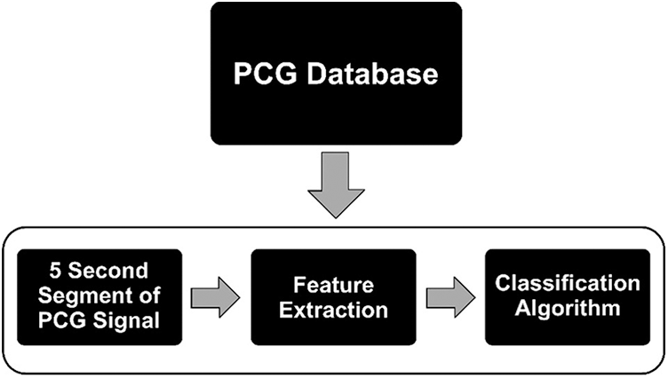
Figure 3: Generic steps involved in heart sound classification w.r.t. machine learning model
Various machine learning models can be used for classifying the heart sound, viz. Artificial Neural Networks (ANN), Support Vector Machine (SVM), Decision Tree (DT), Hidden Markov Model (HMM), and Random Forest (RF) [14,15]. Reddy et al. [16] in their study proposed a hybrid OFBAT-rule based fuzzy logic heart disease diagnosis system. There have been seminal reviews contributed by Dwivedi et al. [17], Nabih-Ali et al. [18], and Clifford et al. [19] in the said domain. Besides, the Convolutional Neural Networks (CNNs) have also been in practice since the last decade for solving the classification problems. CNN requires high computational power as it learns all features from the scratch to provide the final results [20]. It has been found that the concept of transfer learning emphasizes on applying the facts understood while resolving one category of problems to a different, but allied domain. This approach may be a better choice over CNNs as it requires comparatively less computational power. However, transfer learning has only been sparsely reported and hasn't been given a thorough consideration for categorizing the PCG signals. Reddy et al. [21] in their study proposed a novel rough set based method for feature selection and fuzzy rule based method for diagnosing heart disease.
1.3 Focus and Contribution of This Study
Through the survey of related papers that appeared during the period 1999–2019 [17–19], it was observed that the repeating pattern-based spectrograms had not been used for classifying the human heart sounds into normal or abnormal. In the domain of PCG signals, the spectrograms can be used in many verticals like transfer learning, repeating pattern-based spectrograms, textural-based feature extraction from the spectrograms, and amalgamation of spectrograms with either chromagram or scalogram, etc. Where, a spectrogram represents the signal power, or “loudness,” of a signal over time at different frequencies in a specific waveform. Scalograms plot the absolute value of a signal's continuous wavelet transform (CWT) as a function of time and frequency. The chromagram is a time-frequency translation of a signal into a temporally changing precursor of pitch. The research in the domain of acoustics and spectrograms is contemporary and many customizations can be done as an add-on to achieve better results. Arora et al., in their work [22], had used the spectrograms to classify the heart sound signals using machine learning models on the textural-based features extracted from the spectrogram. Whereas, this research work has by-passed the extra step related to feature extraction; and repeating pattern-based spectrograms have been used directly in transfer learning-based models. The pre-trained transfer learning models, viz. ResNet, VGG, Xception, MobileNet, DenseNet, and InceptionV3 have been taken for classifying the spectrograms. By deploying techniques such as data augmentation, overfitting in the classifier has been avoided. The proposed approach has been validated using the PhysioNet 2016 [23] and PASCAL 2011 [24] benchmark datasets. There were 2575 samples of normal and 665 samples of abnormal class in PhysioNet 2016 dataset, whereas 262 samples of normal and 92 samples abnormal class in PASCAL 2011 dataset. For both the benchmarks, 80% of the dataset has been used for training, while the remaining 20% for testing the model's performance.
2 Transfer Learning and Work Related to PCG
Humans are able to acquire knowledge from one task and transfer/apply it to perform more complicated tasks (such as from walking to running). Similarly, transfer learning (or transferability) refers to the training of a machine learning model on some problem domain and applying it for solving the concerns in different but related areas. Here, in this process, the pre-trained neural networks have been amended by replacing their last layer with two fully connected layers followed by a Sigmoid function to classify the repeating pattern-based spectrograms. Transfer learning tends to improve traditional machine learning/deep learning (CNNs) by transferring knowledge in the form of features learned from training on one problem domain and deploy it to another related domain(s) [25]. Fig. 4 illustrates the working of transfer learning.
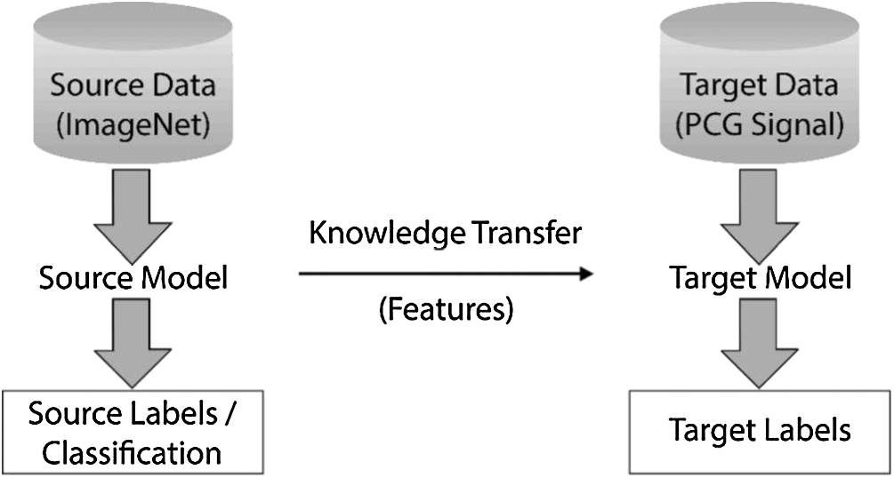
Figure 4: Basic methodology involved in the process of transfer learning
Some of the known pre-trained networks are ResNet, VGG, Xception, MobileNet, DenseNet, and InceptionV3. All these networks have been trained on the ImageNet database and designed to categorize images into 1000 classes [26]. Features such as edge detection and shape detection learned by the pre-trained source model on the ImageNet dataset have been transferred to the target model for their further fine-tuning to classify the PCG signals. While the initial layers have focused on lower-level feature extraction, viz. edge detection and colour blob detectors, the later layers have been customized to be more specific for the details in the dataset under consideration [27].
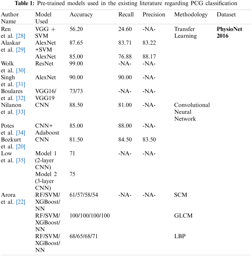
Boulares et al. [32] applied transfer learning approach to recognize cardiovascular diseases using PCG signals from PASCAL 2011 benchmark dataset. Ren et al. [28] and Wolk et al. [30] explored the use of transfer learning for classifying the PCG signals. Ren et al. [28] converted the PCG signals into a scalogram by using a wavelet transformation. These scalograms were fed to a pre-trained VGG16 model for the classification. Nonetheless, the mean accuracy achieved by Ren et al. [28] was only 56.20%, which was not sufficient for real-life applications. Wolk et al. [30] converted the PCG signals into spectrograms which further underwent a basic data augmentation, and were finally fed into a pre-trained convolutional network for classification. Wok et al. The researchers reported a testing accuracy of 99.00%. However, they used the validation dataset which was a part of the training dataset, to validate their model's performance, resulting in over-fitting of the model. Alaskar et al. [29] pre-processed the raw PCG signals to filter the noise and get segmented PCG signals. The PCG scalograms were obtained by applying Cosine Wavelet Transforms (CWT) to these signals. The researchers used pre-trained AlexNet [36] to extract the features and passed them to the SVM classifiers. The result was again fed to AlexNet as an end-to-end learning classifier. Tab. 1 presents the accuracy, recall and precision values obtained from the various pre-trained models deployed at PhysioNet 2016 dataset used for classifying heart sound signals as normal and abnormal.
3 Spectrograms with Repeating Patterns
The spectrogram is a visual depiction of sound. The horizontal bars on the spectrogram represent time; and the vertical bars show frequency. A ‘spectrogram’ is generated from a collection of overlapping windows obtained from the signal and evaluated by computing the Fast Fourier Transform. The method of splitting the signal in small, fixed-size portions and then applying Fourier transforms on them individually is called Short-time Fourier transform (STFT). Then, the spectrograms are measured as the (squared) complex magnitude of the STFT. Spectrograms fall within the domain of images and can be used to discern sounds by means of machine learning models. A distinctive type of spectrogram depicting PCG beats and noisy backgrounds was chosen in this analysis as the input for the Transfer Learning models [37]. Spectrogram exhibited in Fig. 5 explains the relationship between frequency and time for the heart sound signal [13,38].
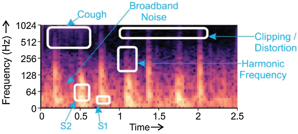
Figure 5: Depiction of S1 and S2 heart sounds, harmonic frequency, broadband noise, and clipping/distortion in a PCG
Fig. 5 displays the components
Spectrograms can accommodate intermittent repeated components, including the quickly changing repeating patterns w.r.t. foreground/background of an audio signal [39]. Fig. 6a displays the beats derived from PCG; the persistent noise background is seen in Figs. 6b, and 6c indicates the incidence of heartbeats.
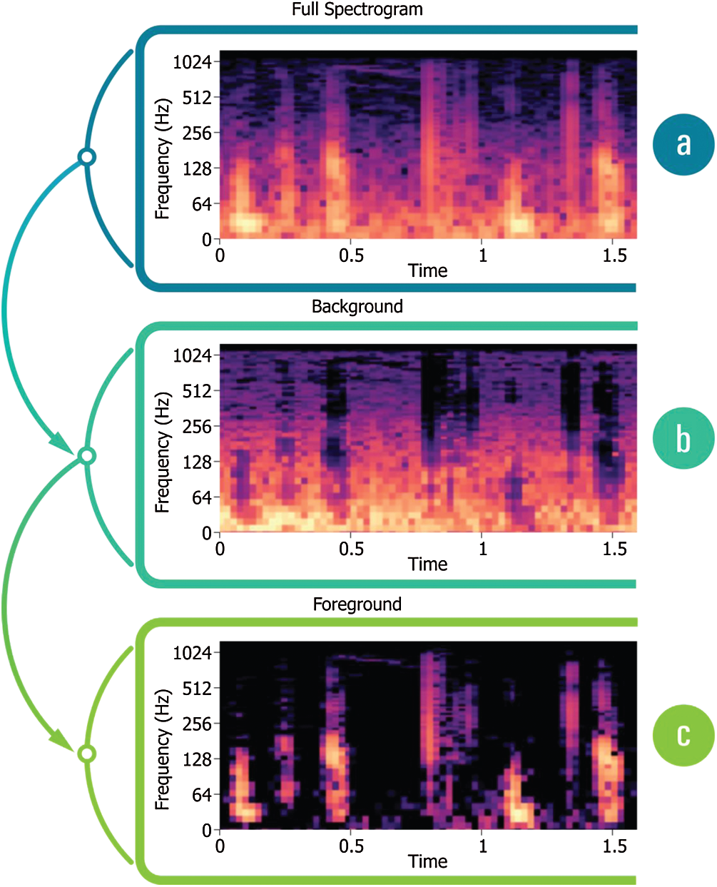
Figure 6: (a) Spectrogram derived from PCG, (b) PCG Spectrogram with a noisy background, (c) Spectrogram displaying
The steps taken into consideration for categorizing heart sound signals as normal or abnormal is highlighted in Fig. 7. PCG signals were taken from the PhysioNet 2016 and PASCAL 2011 datasets and converted into respective spectrograms. The benchmark dataset PhysioNet2016 holds the records used in the PhysioNet/CinC Challenge 2016. Heart sound samples were obtained from a variety of sources around the globe, in both clinical and nonclinical settings, from both safe and pathological individuals. PASCAL 2011 dataset was collected from two sources: (A) the general population using the iStethoscope Pro iPhone software (Dataset A), and (B) a clinic experiment in hospitals using the DigiScope wireless stethoscope (Dataset B).
In this research work, the proposed methodology has been implemented using Python (Version 3.7.6), Keras (Version 2.3.1), NumPy (Version 1.18.2), Tensor Flow (Version 1.15.2), Librosa (Version 0.7.0), SciPy (Version 1.4.1). The experimental work has been conducted using Intel Core i7 processor, 8 GB RAM, and Windows 10 Pro operating system. Repeat patterns were established with a similarity matrix. These patterns were further filtered to generate spectrograms with patterns that denoted unrepeated noisy PCG signals. A soft mask had been added to the background spectrum to remove noise from the heart sound signal.
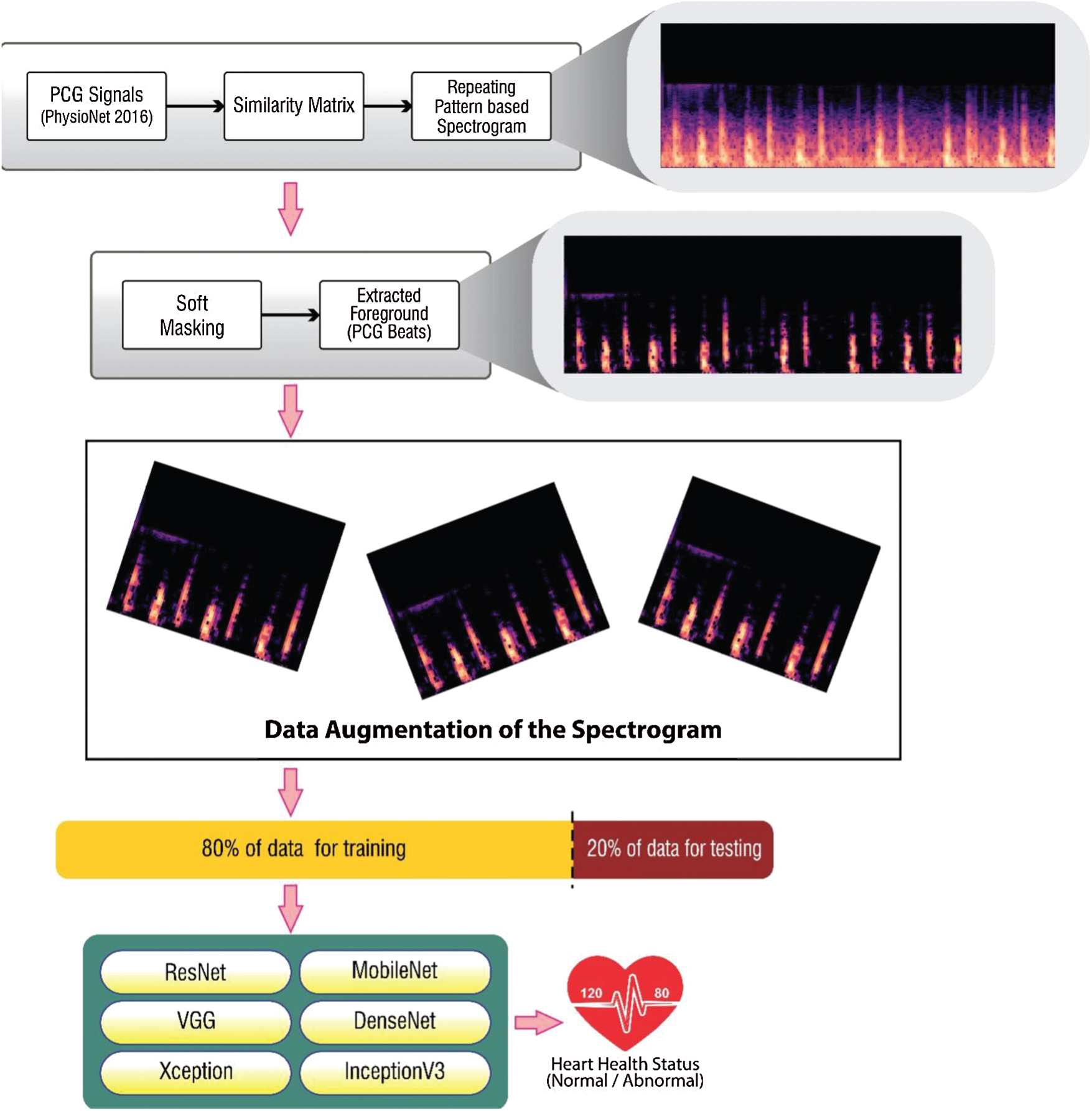
Figure 7: Methodology for classification of PCG signals using repeating pattern-based spectrogram
4.1 Modelling the Spectrogram Using Similarity Matrix and Soft-Mask
The similarity matrix accurately determined cosine similarity among transposed spectrograms and normal spectrograms of the PCG signal [40]. With quarterly overlapping N hamming sample length windows, the transition of STFT for the PCG (
• Using the cosine similarity measure, a similarity matrix S was computed from V.
• For each frame in S, the frequency of unique repetitive patterns was identified.
• Median of frames in V had been computed for each frequency channel over all the repeating frames of W.
A sparse time-frequency (TF) depiction of PCG signal was contrasted with TF depiction of background sound element. The median filter detected minor changes in the intervals of TF, and deleted the intervals with great variations (outliers) from the repetitive patterns. Soft time-frequency masking was implemented to distinguish speech signals from noise-in-speech mixtures. The spectrogram depicting heart sound with noise (
Two fully connected layers have been added to the convolutional bases. These fully connected layers extract the domain-specific features from the repeating pattern-based spectrograms here in this research work. The hyper-parameter optimization has been conducted on the original dataset using a 5-fold cross-validation validation technique. Various parameters like batch size, layer size, regularization have been experimented with for various values. The combination of
Augmentation of data is done to produce fresh training samples artificially from the existing training data. Domain-specific techniques have been applied to existing examples from the training data to create novel training samples. The prediction accuracy of deep learning models is dependent on the amount and the diversity of data available during training. Data augmentation not only addresses both these requirements, but it can also be used to address the class imbalance problem in classification tasks. Imaging data augmentation is a documented method of data increase in which converted image copies are used with original image in a training dataset for original class. Various transforms have been tried by the researchers which mainly include shifting, flipping, zooming among range of image manipulation operations.
Data augmentation can be effectively used to train the deep learning models in complex applications. Modern deep learning algorithms (e.g., CNN) can learn location-invariant features in the image. Augmentation boosts this transform invariant approach to learning transform invariant features such as ordering (Left
5 Discussion on Experimentation Results
The PhysioNet 2016 and PASCAL 2011 benchmark datasets have been used here for experimentation with transfer learning models.
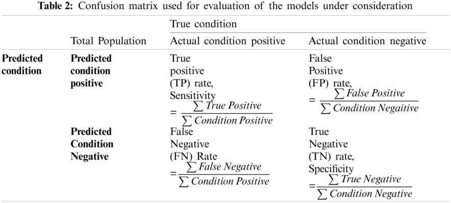
Tab. 2 shows a confusion matrix providing the details about sensitivity, precision, recall, and fall-out. The matrix reflects the performance of a model in machine learning. Columns in this matrix represent real class instances, while the rows reflect instances in an anticipated class. The proportion of positive cases predicted to be positive is referred to as sensitivity. The proportion of real negatives reported to be negative is used to calculate the specificity. A false positive is a classification mistake in which a test outcome falsely suggests the existence of a disorder that does not exist in fact. Whereas, false negatives are negative outcomes that the model predicted incorrectly. In context of cardiac arrhythmia true positive indicates the count of subjects that suffer from some aliment and model has correctly identified them. True negative is the count where the model correctly identified the normal subjects. False positive is the count where the proposed model has predicted normal subjects as patients. False negative refers to the count of abnormal subjects that are predicted as normal.
For the purpose of this research, accuracy, precision, recall and F1-score have been used to form the evaluation criteria. Accuracy is the indicator of all well-identified incidents. Precision-Recall is a powerful predictive efficiency predictor where datasets are quite imbalanced.
F1-score may be a better metric to use, if we need to seek a balance between Precision and Recall, especially where there is an unequal class distribution. F1-score has also been used where the False Negatives and False Positives are crucial.
5.2 Comparison Among Transfer Learning Models
The transfer learning models have been trained using the holdout validation technique, taking
Tabs. 3 and 4 presents the accuracy, recall, precision, and F1-scores as obtained for the PhysioNet 2016 database with and without data augmentation respectively. The results for the MobileNet, Xception, VGG16, ResNet, DenseNet and InceptionV3 have been listed and computed on 20% of the base dataset reserved for validation of the model. DenseNet has appeared with the highest accuracy in comparison to its peer approaches. Fig. 8 presents the plots drawn for the accuracy, recall, precision, and F1-score obtained on the PhysioNet 2016 benchmark dataset.
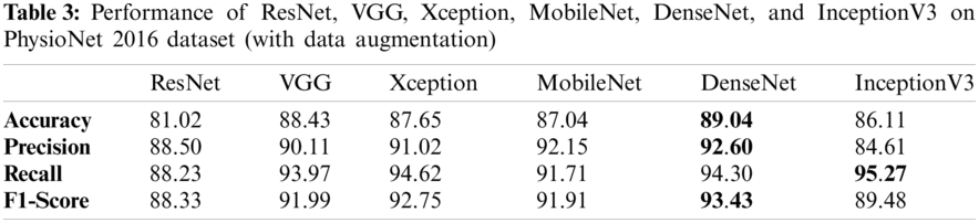
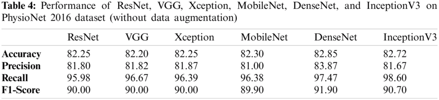
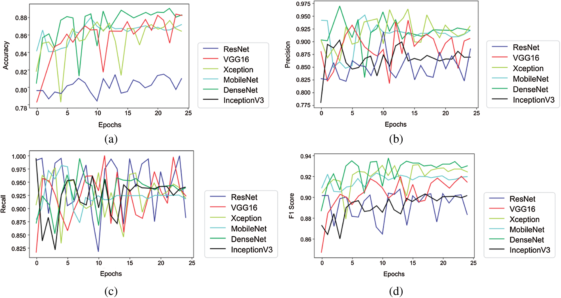
Figure 8: Plots obtained for various evaluation parameters, viz. ResNet, VGG16, Xception, MobileNet, DenseNet and InceptionV3 on PhysioNet 2016 dataset
Tabs. 5 and 6 exhibit the accuracy, recall, precision, and F1-scores as obtained for the PASCAL 2011 database with and without data augmentation respectively. The results for the MobileNet, Xception, VGG16, ResNet, DenseNet and InceptionV3 have been listed and computed on 20% of the base dataset reserved for validation of the model. VGG16 has appeared with the highest accuracy in comparison to other approaches. Fig. 9 shows the plots for the accuracy, recall, precision, and F1-scores obtained on the PASCAL 2011 benchmark dataset.
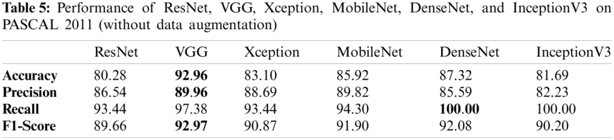
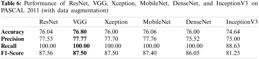
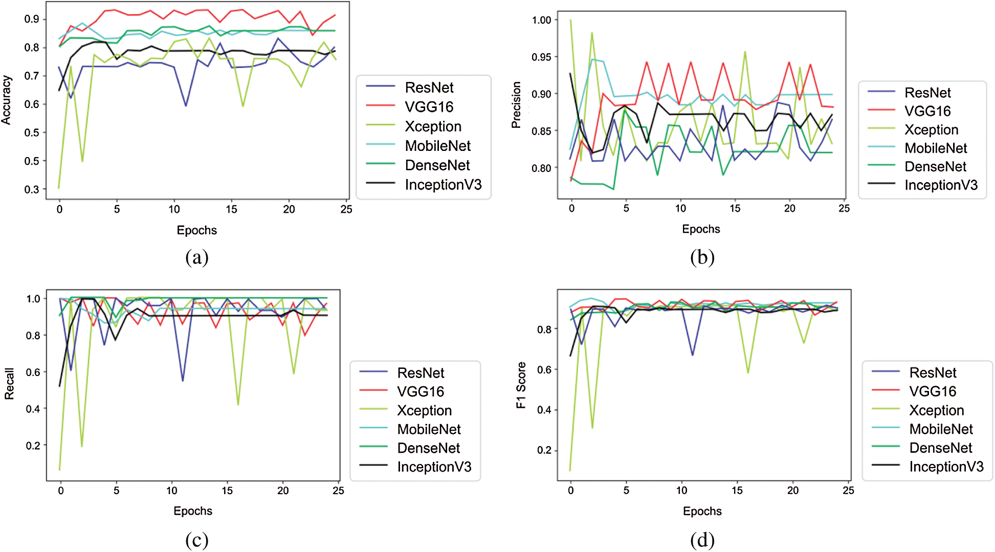
Figure 9: Plots obtained for various evaluation parameters, viz. ResNet, VGG16, Xception, MobileNet, DenseNet and InceptionV3 on PASCAL 2011 dataset
It is evident from Tabs. 3–6 that results obtained after applying augmentation are better as compared to the results without applying the data augmentation operation. Due to skewed class distribution of the benchmark datasets, both accuracy and F1-score have been used for comparison [44,45].
A new type of spectrogram, i.e., repetition-based spectrogram has been used as an input for the transfer learning models. At PhysioNet 2016 dataset, the DenseNet has outperformed all its peers; whereas, for PASCAL 2011 dataset, VGG16 has performed excellently. The approach handled by the authors in this work has considered only one depiction of PCG signals, i.e., spectrograms, which is an image representation of sound signals in time-frequency domain. The proposed approach can be enhanced further using chromagrams, melspectrograms and scalograms in conjunction with spectrogram for a PCG sound signal, as these can depict the sound in the different pitch classes. In future, the accuracy of the prediction model can be improved by using an ensemble of the model that had the best performance at PhysioNet 2016 and PASCAL 2011 dataset (i.e., DenseNet and/or VGG) with Boosting algorithm like XGBoost.
Author Contributions: Conceptualization, Vinay Arora and Karun Verma; Data curation, Rohan Leekha and Kashish Bhatia; Formal analysis, Kyungroul Lee; Investigation, Karun Verma; Methodology, Vinay Arora and Kyungroul Lee; Project administration, Vinay Arora and Karun Verma; Resources, Kyungroul Lee; Software, Rohan Leekha, Takshi Gupta and Kashish Bhatia; Validation, Karun Verma, Rohan Leekha and Chang Choi; Visualization, Vinay Arora, Rohan Leekha and Chang Choi; Writing – original draft, Vinay Arora; Writing – review & editing, Vinay Arora and Karun Verma.
Funding Statement: This work was supported by the National Research Foundation of Korea(NRF) Grant Funded by the Korea government (Ministry of Science and ICT) (No. 2017R1E1A1A01077913) and by the Institute of Information & Communications Technology Planning & Evaluation (IITP) funded by the Korea Government (MSIT) (Development of Smart Signage Technology for Automatic Classification of Untact Examination and Patient Status Based on AI) under Grant 2020-0-01907.
Conflicts of Interest: The authors declare that they have no conflicts of interest to report regarding the present study.
1. V. Puri, A. Kataria and V. Sharma, “Artificial intelligence-powered decentralized framework for internet of things in healthcare 4.0,” Transactions on Emerging Telecommunications Technologies, pp. 1–18, 2021. https://doi.org/10.1002/ett.4245. [Google Scholar]
2. I. You, K. Yim, V. Sharma, G. Choudhary, I. R. Chen et al., “Misbehavior detection of embedded IoT devices in medical cyber physical systems,” in Proc.—2018 IEEE/ACM Int. Conf. on Connected Health: Applications, Systems and Engineering Technologies, CHASE 2018, Washington DC, USA, pp. 88–93, 2019. [Google Scholar]
3. V. Stantchev, A. Barnawi, S. Ghulam, J. Schubert and G. Tamm, “Smart items, fog and cloud computing as enablers of servitization in healthcare,” Sensors & Transducers, vol. 185, no. 2, pp. 121–128, 2015. [Google Scholar]
4. S. Tuli, N. Basumatary, S. S. Gill, M. Kahani, R. C. Arya et al., “Healthfog: An ensemble deep learning based smart healthcare system for automatic diagnosis of heart diseases in integrated IoT and fog computing environments,” Future Generation Computer Systems, vol. 104, pp. 187–200, 2020. [Google Scholar]
5. T. N. Gia, M. Jiang, A. M. Rahmani, T. Westerlund, P. Liljeberg et al., “Fog computing in healthcare internet of things: A case study on ECG feature extraction,” in Proc.—15th IEEE Int. Conf. on Computer and Information Technology, CIT 2015, Liverpool, United Kingdom, pp. 356–363, 2015. [Google Scholar]
6. I. S. M. Isa, M. O. I. Musa, T. E. H. El-Gorashi, A. Q. Lawey and J. M. H. Elmirghani, “Energy efficiency of fog computing health monitoring applications,” in 2018 20th Int. Conf. on Transparent Optical Networks, Bucharest, Romania, pp. 1–5, 2018. [Google Scholar]
7. H. Yang, C. Kan, A. Krall and D. Finke, “Network modeling and internet of things for smart and connected health systems—A case study for smart heart health monitoring and management,” IISE Transactions on Healthcare Systems Engineering, vol. 10, no. 3, pp. 1–13, 2020. [Google Scholar]
8. M. A. G. Santos, R. Munoz, R. Olivares, P. P. Rebouças Filho, J. Del Ser et al., “Online heart monitoring systems on the internet of health things environments: A survey, a reference model and an outlook,” Information Fusion, vol. 53, pp. 222–239, 2020. [Google Scholar]
9. T. Chakrabarti, S. Saha, S. Roy and I. Chel, “Phonocardiogram signal analysis-practices, trends and challenges: A critical review,” in 2015 Int. Conf. and Workshop on Computing and Communication, Vancouver, BC, Canada, pp. 1–4, 2015. [Google Scholar]
10. M. Malcangi, M. Riva and K. Ouazzane, “Hard and soft computing methods for capturing and processing phonocardiogram,” International Journal of Circuits, Systems and Signal Processing, vol. 7, no. 1, pp. 34–41, 2013. [Google Scholar]
11. S. M. Debbal and F. Bereksi-Reguig, “Filtering and classification of phonocardiogram signals using wavelet transform,” Journal of Medical Engineering & Technology, vol. 32, no. 1, pp. 53–65, 2008. [Google Scholar]
12. F. Alias, J. Socoró and X. Sevillano, “A review of physical and perceptual feature extraction techniques for speech, music and environmental sounds,” Applied Sciences, vol. 6, no. 5, p. 143, 2016. [Google Scholar]
13. L. Wyse, “Audio spectrogram representations for processing with convolutional neural networks,” in Proc. of the First Int. Workshop on Deep Learning and Music Joint with IJCNN, Anchorage, US, vol. 1, no. 1, pp. 37–41, 2017. [Google Scholar]
14. N. E. Singh-Miller and N. Singh-Miller, “Using spectral acoustic features to identify abnormal heart sounds,” in 2016 Computing in Cardiology Conf., Vancouver, BC, pp. 557–560, 2016. [Google Scholar]
15. D. Patel, K. Srinivasan, C.-Y. Chang, T. Gupta and A. Kataria, “Network anomaly detection inside consumer networks—A hybrid approach,” Electronics, vol. 9, no. 6, pp. 923, 2020. [Google Scholar]
16. G. T. Reddy and N. Khare, “An efficient system for heart disease prediction using hybrid OFBAT with rule-based fuzzy logic model,” Journal of Circuits, Systems and Computers, vol. 26, no. 4, pp. 1750061, 2017. [Google Scholar]
17. A. K. Dwivedi, S. A. Imtiaz and E. Rodriguez-Villegas, “Algorithms for automatic analysis and classification of heart sounds---A systematic review,” IEEE Access, vol. 7, pp. 8316–8345, 2018. [Google Scholar]
18. M. Nabih-Ali, E.-S. A. El-Dahshan and A. S. Yahia, “A review of intelligent systems for heart sound signal analysis,” Journal of Medical Engineering and Technology, vol. 41, no. 7, pp. 553–563, 2017. [Google Scholar]
19. G. D. Clifford, C. Liu, B. Moody, J. Millet, S. Schmidt et al., “Recent advances in heart sound analysis,” Physiological Measurement, vol. 38, no. 8, pp. E10–E25, 2017. [Google Scholar]
20. B. Bozkurt, I. Germanakis and Y. Stylianou, “A study of time-frequency features for CNN-based automatic heart sound classification for pathology detection,” Computers in Biology and Medicine, vol. 100, pp. 132–143, 2018. [Google Scholar]
21. G. T. Reddy, M. P. K. Reddy, K. Lakshmanna, D. S. Rajput, R. Kaluri et al., “Hybrid genetic algorithm and a fuzzy logic classifier for heart disease diagnosis,” Evolutionary Intelligence, vol. 13, no. 2, pp. 185–196, 2020. [Google Scholar]
22. V. Arora, E. Y.-K. Ng, R. S. Leekha, K. Verma, T. Gupta et al., “Health of things model for classifying human heart sound signals using Co-occurrence matrix and spectrogram,” Journal of Mechanics in Medicine and Biology, vol. 20, no. 6, pp. 2050040, 2020. [Google Scholar]
23. C. Liu, D. Springer, Q. Li, B. Moody, R. A. Juan et al., “An open access database for the evaluation of heart sound algorithms,” Physiological Measurement, vol. 37, no. 12, pp. 2181, 2016. [Google Scholar]
24. S.-W. Deng and J.-Q. Han, “Towards heart sound classification without segmentation via autocorrelation feature and diffusion maps,” Future Generation Computer Systems, vol. 60, pp. 13–21, 2016. [Google Scholar]
25. D. Elavarasan, D. R. Vincent, V. Sharma, A. Y. Zomaya and K. Srinivasan, “Forecasting yield by integrating agrarian factors and machine learning models: A survey,” Computers and Electronics in Agriculture, vol. 155, Amsterdam: Elsevier B.V., pp. 257–282, 2018. [Google Scholar]
26. C. Tai, T. Xiao, Y. Zhang, X. Wang and E. Weinan, “Convolutional neural networks with low-rank regularization,” in 2016 Int. Conf. on Learning Representations, ICLR (PosterSan Juan, Puerto Rico, arXiv preprint arXiv: 1511.06067, 2016. [Google Scholar]
27. A. Karpathy, G. Timnit, K. Zakka, B. Shyamal, J. Jhonson et al., “Cs231n convolutional neural networks for visual recognition,” 2016. [Online]. Available: https://cs231n.github.io/. [Accessed: 12-May-2020]. [Google Scholar]
28. Z. Ren, N. Cummins, V. Pandit, J. Han, K. Qian et al., “Learning image-based representations for heart sound classification,” in Proc. of the 2018 Int. Conf. on Digital Health, Lyon, France, pp. 143–147, 2018. [Google Scholar]
29. H. Alaskar, N. Alzhrani, A. Hussain and F. Almarshed, “The implementation of pretrained alexNet on PCG classification,” in Int. Conf. on Intelligent Computing, Nanchang, China, pp. 784–794, 2019. [Google Scholar]
30. A. Wołk, “Early and remote detection of possible heartbeat problems with convolutional neural networks and multipart interactive training,” IEEE Access, vol. 7, pp. 145921–145927, 2019. [Google Scholar]
31. S. A. Singh, S. Majumder and M. Mishra, “Classification of short unsegmented heart sound based on deep learning,” in 2019 IEEE Int. Instrumentation and Measurement Technology Conf., Auckland, New Zealand, pp. 1–6, 2019. [Google Scholar]
32. M. Boulares, T. Alafif and A. Barnawi, “Transfer learning benchmark for cardiovascular disease recognition,” IEEE Access, vol. 8, pp. 109475–109491, 2020. [Google Scholar]
33. T. Nilanon, J. Yao, J. Hao, S. Purushotham and Y. Liu, “Normal/abnormal heart sound recordings classification using convolutional neural network,” in 2016 Computing in Cardiology Conf., Vancouver, BC, Canada, pp. 585–588, 2016. [Google Scholar]
34. C. Potes, S. Parvaneh, A. Rahman and B. Conroy, “Ensemble of feature-based and deep learning-based classifiers for detection of abnormal heart sounds,” in 2016 Computing in Cardiology Conf., Vancouver, BC, Canada, pp. 621–624, 2016. [Google Scholar]
35. J. X. Low and K. W. Choo, “Automatic classification of periodic heart sounds using convolutional neural network,” World Academy Science Engineering and Technology, International Journal of Electrical and Computer Engineering, vol. 5, pp. 100–105, 2018. [Google Scholar]
36. S. Das, “CNN architectures: LeNet, alexNet, VGG, googLeNet, resNet and more…, ” Nov-2017. [Online]. Available: https://medium.com/analytics-vidhya/cnns-architectures-lenet-alexnet-vgg-googlenet-resnet-and-more-666091488df5. [Accessed: 12-Jun-2020]. [Google Scholar]
37. C.-L. Hsu and J.-S. R. Jang, “On the improvement of singing voice separation for monaural recordings using the MIR-1K dataset,” IEEE Transactions on Audio, Speech and Language Processing, vol. 18, no. 2, pp. 310–319, 2009. [Google Scholar]
38. Y. Wu, H. Mao and Z. Yi, “Audio classification using attention-augmented convolutional neural network,” Knowledge-Based Systems, vol. 161, pp. 90–100, 2018. [Google Scholar]
39. Z. Rafii and B. Pardo, “Music/Voice separation using the similarity matrix,” in Int. Society of Music Information Retrieval Conf., Porto, Portugal, pp. 583–588, 2012. [Google Scholar]
40. J. Zheng, C. Lu, C. Hao, D. Chen and D. Guo, “Improving the generalization ability of deep neural networks for cross-domain visual recognition,” IEEE Transactions on Cognitive and Developmental Systems, pp. 1–15, 2020. https://doi.org/10.1109/TCDS.2020.2965166. [Google Scholar]
41. B. McFee, C. Raffel, D. Liang, D. P. W. Ellis, M. McVicar et al., “Librosa: Audio and music signal analysis in python,” in Proc. of the 14th Python in Science Conf., Austin, Texas, vol. 8, pp. 18–25, 2015. [Google Scholar]
42. G. T. Reddy, S. Bhattacharya, P. K. R. Maddikunta, S. Hakak, W. Z. Khan et al., “Antlion re-sampling based deep neural network model for classification of imbalanced multimodal stroke dataset,” Multimedia Tools and Applications, vol. 9, pp. 1–25, 2020. [Google Scholar]
43. F. Chollet, “Keras: Deep learning library for theano and tensorflow,” 2015. [Online]. Available: https://keras.io. [Accessed: 26-Jun-2020]. [Google Scholar]
44. H. Altinger, S. Herbold, F. Schneemann, J. Grabowski and F. Wotawa, “Performance tuning for automotive software fault prediction,” in 2017 IEEE 24th Int. Conf. on Software Analysis, Evolution and Reengineering, Klangenfurt, Austria, pp. 526–530, 2017. [Google Scholar]
45. R. Joshi, “Accuracy, precision, recall & F1 score: Interpretation of performance measures-exsilio blog,” 2016-09-09, 2016. [Online]. Available: https://blog.exsilio.com/all/accuracy-precision-recall-f1-score-interpretation-of-performance-measures/. [Accessed: 18-Aug-2020]. [Google Scholar]
 | This work is licensed under a Creative Commons Attribution 4.0 International License, which permits unrestricted use, distribution, and reproduction in any medium, provided the original work is properly cited. |