Computers, Materials & Continua DOI:10.32604/cmc.2021.019900
Article

Application of Grey Model and Neural Network in Financial Revenue Forecast

Yifu Sheng1, Jianjun Zhang1,*, Wenwu Tan1, Jiang Wu1, Haijun Lin1, Guang Sun2 and Peng Guo3

1College of Engineering and Design, Hunan Normal University, Changsha, 410081, China
2Big Data Institute, Hunan University of Finance and Economics, Changsha, 410205, China
3University Malaysia Sabah, Sabah, 88400, Malaysia
*Corresponding Author: Jianjun Zhang. Email: jianjun998@163.com
Received: 30 April 2021; Accepted: 12 June 2021

Abstract: There are many influencing factors of fiscal revenue, and traditional forecasting methods cannot handle the feature dimensions well, which leads to serious over-fitting of the forecast results and unable to make a good estimate of the true future trend. The grey neural network model fused with Lasso regression is a comprehensive prediction model that combines the grey prediction model and the BP neural network model after dimensionality reduction using Lasso. It can reduce the dimensionality of the original data, make separate predictions for each explanatory variable, and then use neural networks to make multivariate predictions, thereby making up for the shortcomings of traditional methods of insufficient prediction accuracy. In this paper, we took the financial revenue data of China’s Hunan Province from 2005 to 2019 as the object of analysis. Firstly, we used Lasso regression to reduce the dimensionality of the data. Because the grey prediction model has the excellent predictive performance for small data volumes, then we chose the grey prediction model to obtain the predicted values of all explanatory variables in 2020, 2021 by using the data of 2005–2019. Finally, considering that fiscal revenue is affected by many factors, we applied the BP neural network, which has a good effect on multiple inputs, to make the final forecast of fiscal revenue. The experimental results show that the combined model has a good effect in financial revenue forecasting.

Keywords: Fiscal revenue; lasso regression; gray prediction model; BP neural network

1  Introduction

Local fiscal revenue is an important part of national fiscal revenue. Scientific and reasonable forecasting of local fiscal revenue is of great significance for overcoming the arbitrariness and blindness of the annual local budget scale and correctly handling the relationship between local finance and economy [1]. The analysis and forecast of fiscal revenue has always been a hot topic for many scholars, and the choice of variables is the first problem they face. In 1974, Japanese statistician Akaike [2] proposed the AIC information criterion, which meant the emergence of the concept of variable selection, but this method lacks stability in variable selection. In order to solve this problem, in 1996, Tibshirani [3] proposed the Lasso method based on the Ridge Regression method [4] and the Nonegtive Garrote method [5], so as to achieve variable selection and increase interpretability. Li [6] used the Lasso method when conducting forecast analysis on Gansu Province's fiscal revenue. In 1982, Professor Deng Julong, a well-known Chinese scholar, published a paper titled ‘The control problems of grey systems’ in the journal “Systems and Control Communications,” marking the official birth of the grey system theory. Once this theory was put forward, it attracted the attention of many scholars [7]. Peng [8] used the gray model to predict and analyze the national fiscal revenue. The most commonly used gray model is the GM(1,1) model [9]. This model can generate gray on the original data, mine the unobvious laws in the data and get the data with increasing trend, then model and analyze the regular data, and finally realize the simulation and prediction of the model through gray restoration. Yuan et al. [10] chose the GM(1,1) residual model to modify the traditional GM(1,1) and used it to predict and analyze fiscal revenue.

In recent years, with the continuous development of the cloud computing technology, neural network technology has also ushered in a new wave, and has achieved good results in many fields, such as data analysis [11], spam detection [12], image recognition [13], and automatic driving [14]. Fang et al. [15] studied the problem of the ARMA-BP neural network combination model for forecasting the fiscal revenue. Jiang et al. [16] gave a Lasso-GRNN neural network model for the local fiscal revenue, taking into account the complex nonlinear relationship of its influencing factors. Chen et al. [17] proposed a deep network prediction model based on BP neural network. The fiscal revenue is affected by multiple factors such as economy and policy. A single model can only obtain part of the information on data changes, and the prediction accuracy is relatively low. Based on the above research, in this paper, a model, combining the GM(1,1) and the BP neural network, was proposed to predict the local fiscal revenue of Hunan Province in 2020 and 2021. Compared with a single prediction model GM(1,1), the results show that the combined model not only improves the prediction accuracy, but also provides a basis for the complex, dynamic and accurate forecast of fiscal revenue.

2  Related Works

2.1 Variable Selection Model

2.1.1 Lasso Regression Theory and Algorithm

Lasso regression is a compression estimation method. In order to achieve compression of the model regression coefficient, its core principle is to constrain the absolute values’ sum of the parameters to be estimated within a certain preset threshold by constructing a penalty function in the model [18]. When this threshold is set to a very small number, some regression coefficients could be compressed to 0, then variables with a coefficient of 0 could be eliminated, thereby achieving variable screening. Reducing irrelevant coefficients can enhance the interpretability of the model.

The Lasso method is equivalent to adding the L1 penalty term to the ordinary linear model:

β^lasso=argmin(‖Y−Xβ‖2+λ∑j=1d|βj|) (1)

The equivalent is:

β^lasso=argmin‖Y−Xβ‖2, s.t. ∑j=1d|βj|≤t,λ≥0 (2)

where t is called the adjustment factor, corresponds to λ one-to-one. Lett0=∑j=1d|β^(OLS)|. When t<t0, some coefficients will be compressed to 0, resulting in sparseness, thereby reducing the dimension of X and achieving the effect of variable screening.

2.1.2 Ridge Regression Theory and Algorithm

In the ordinary linear model, when the covariates X(f) are independent of each other, the parameter β obtained by ordinary least squares estimation has good properties, and β^OLS is an unbiased estimate. Among all unbiased estimates, β^OLS has the smallest variance. But when the dimension of the covariate X(f) increases, the correlation will increase, and matrix X will no longer be a full-rank matrix, which is commonly called an ill-conditioned matrix. When the matrix X is ill-conditioned, XTX is a singular matrix. At this time, the β^OLS variance is the smallest, but the value is large, resulting in low accuracy and instability. In this case, the Ridge regression method is usually used.

The Ridge method adds a L2 penalty term to the ordinary linear model:

β^Ridge=argmin (‖Y−Xβ‖2+λ∑j=1d|βj|2) (3)

Equivalent to:

β^Ridge=argmin‖Y−Xβ‖2, s.t. ∑j=1d|βj|2≤t,λ≥0 (4)

β^Ridge is a biased estimate of β, and β^Ridge is a proportional compression of the ordinary least squares estimation β^OLS, and it could not compress the non-zero coefficients t to zero.

2.1.3 Comparing Lasso Regression with Ridge Regression

The difference between Lasso Regression and Ridge regression is shown in Fig. 1. The constraint domain and contour lines of the two methods are described in the figure. The ellipse center point β^ corresponds to the least squares estimation of the linear model. The red ellipse contour represents the squares sum of the model residuals corresponding to λ, and the cyan part below is the constraint domain. The Lasso regression on the left is a square constrained domain, and the Ridge regression on the right is a circular constrained domain. The tangent point between the constraint domain and the contour line is the optimal solution. It can be clearly seen from the figure that the square constraint domain of Lasso regression can easily make the tangent point fall on the coordinate axis, and the variable coefficient could be taken to 0, resulting in sparseness. The circular constraint domain of ridge regression generally does not make the tangent point fall on the coordinate axis, and the variable coefficient could not be compressed to 0, then the variable selection could not be performed. Although ridge regression can also compress the original variable coefficients to a certain extent, it cannot compressed them to 0, so the final model will retain all the variables. On the contrary, Lasso directly compresses the coefficients with less correlation to 0 and proceed directly variable screening.

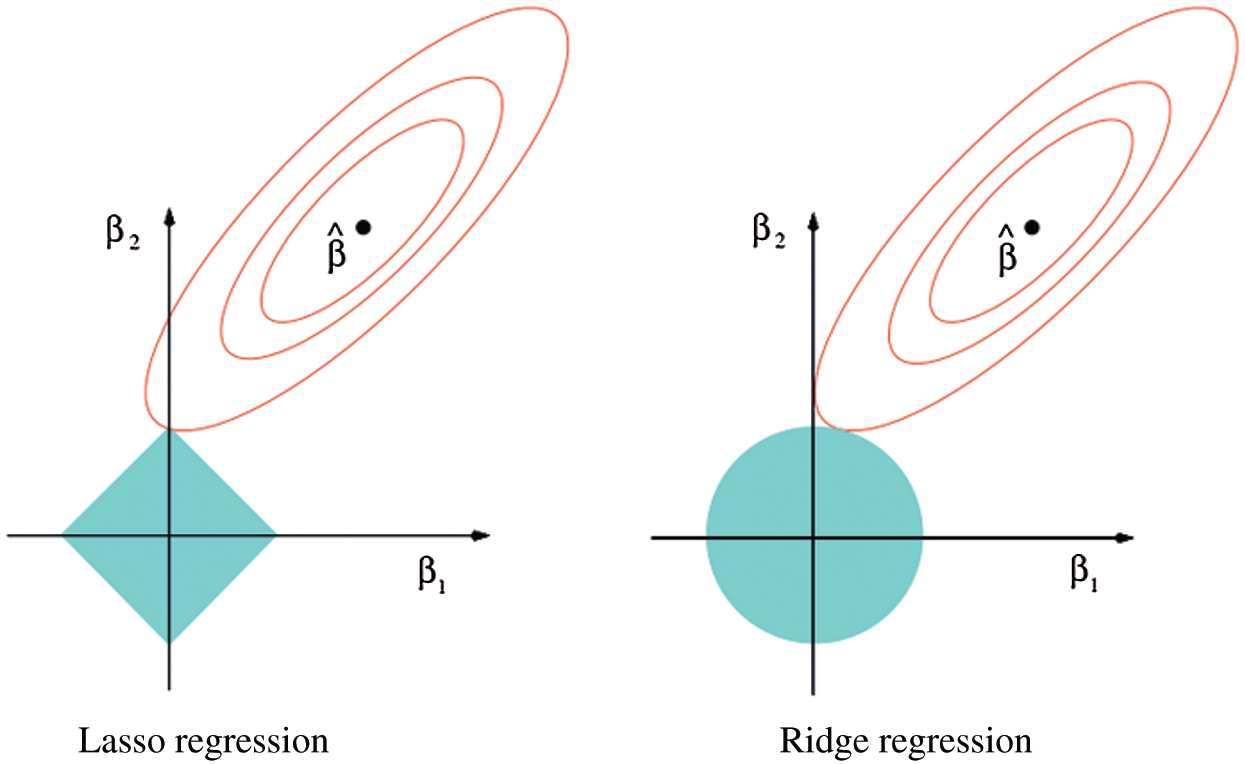
Figure 1: Comparing lasso regression with ridge regression

2.2 Grey System Theory

Grey theory is an emerging edge scientific theory, initiated by the famous Chinese scholar Deng Julong, which aims at "poor information" or "small sample" systems with incomplete information. That is to say, while reflecting the reality, the gray system theory conducts reasonable analysis and in-depth mining of incomplete information, obtains unknown information, and then makes a more accurate description of the overall development law and change trend [19].

2.2.1 Gray Sequence Generation

The information of the gray system is usually chaotic. By generating gray sequence, the method of mining the originally irregular data to explore the change law of the data is called gray generation. Gray generation can adjust the value and nature of the data in the sequence while maintaining the original sequence form, thereby revealing the regularity of the data and weakening the randomness of the data through a certain generation. Gray generation provides the basis and direction for modeling decision-making. It can dig out the hidden nature of the sequence, expose the monotonous increasing trend hidden in the sequence, and turn incomparable sequences into comparable sequences [20].

The commonly used gray sequence generation methods are: Accumulating Generation Operator, Inverse Accumulating Generation Operator, Average-generating Arithmetic Operators, Level Ratio Generation, and Buffer Generation [21]. In this paper, accumulating generation operator and average-generating arithmetic operators are used, and the two generation methods are briefly described below.

Accumulating Generation Operator is the most basic and important generation method of gray theory. Through accumulation, the data characteristics of the original sequence are transformed, and the regularity and predictability of the newly obtained sequence are integrated, thus reducing the randomness of the original sequence. The specific form of the original sequence X(0) is:

X(0)=(x(0)(1),x(0)(2),…,x(0)(n)),∀x(0)(i)∈R+,n∈N (5)

Let:

x(1)(k)=∑k=1kx(0)(i),k=1,2,…,n (6)

So:

X(1)=(x(1)(1),x(1)(2),…,x(1)(n)) (7)

Here X(1) is an Accumulating Generation Operator of X(0). In the same way, any number of cumulative sequences can be derived.

Average-generating Arithmetic Operators includes adjacent generation and non-adjacent generation. Adjacent generation means that when the original sequence is equally spaced, the adjacent data in the sequence are averaged to generate a new data, so the new constructed sequence will be one unit less than the original sequence. Non-adjacent generation means that when the original sequence is not evenly spaced or there are abnormal points in the original data, the mean value of adjacent data is used to replace the abnormal points. It can be used to make up for missing points in the original sequence and construct new data reasonably. The problem of sequence vacancies caused by missing data is solved, and a complete sequence is formed.

As mentioned earlier, the original sequence X(0) expression is:

X(0)=(x(0)(1),x(0)(2),…,x(0)(n)),∀x(0)(i)∈R+,n∈N (8)

Let:

x∗(k)=px(0)(k)+(1−p)x(0)(k−1) (9)

X(∗)=(x(∗)(1),x(∗)(2),…,x(∗)(n)) (10)

Expression p is called the generation coefficient, and the value of the generation coefficient represents different information weights in the new sequence X(∗). The value of p is usually 0.5.

2.2.2 Grey Prediction Model GM(1,1)

The GM(1,1) model is a classic model of gray theory. The two 1s in parentheses represent first-order differential equations and one variable. The GM(1,1) model firstly accumulates the original sequence data, converts the original data to non-negative and non-subtractive ones, establishes a differential equation for the accumulation sequence, uses the least square method to solve the equation coefficients, then predicts the accumulation sequence, and finally restitutes the accumulation sequence to obtain the prediction of the original sequence.

For the original sequence X(0):

X(0)=(x(0)(1),x(0)(2),…,x(0)(n)),∀x(0)(i)∈R+,n∈N (11)

The cumulative form of the gray generation sequence is X(1):

X(1)=(x(1)(1),x(1)(2),…,x(1)(n)),∀x(1)(i)∈R+,n∈N (12)

Let:

x(2)(k)=0.5x(1)(k)+0.5x(1)(k−1),∀x(1)(i)∈X(1) (13)

So there is a sequence of mean values X(2):

X(2)=(x(2)(2),x(2)(3),…,x(2)(n)) (14)

With the above expressions, the original form of the G(1,1) model can be obtained:

x(0)(k)+ax(2)(k)=b(k=2,3,…,n) (15)

a is the development coefficient, and b is the ash effect.

GM(1,1) is solved by using the least square method, and a differential equation will be obtained. This equation is called the whitening equation of GM(1,1). The specific form is as follows:

dx(1)dt+ax(1)=b (16)

Solve the differential equation, and discretize the time response sequence:

x^(1)(k+1)=(x(0)(1)−ba)e−a(k)+ba,k=2,3,…,n (17)

Finally, it can be used to predict the fitted value of the original sequence:

x^(0)(k+1)=x^(1)(k+1)−x^(1)(k),k=2,3,…,n (18)

2.3 Neural Network Theory

The artificial neural network is a calculation model designed to simulate the human brain neural network. It simulates the human brain neural network in terms of structure, realization mechanism and function [22]. An artificial neural network is similar to a biological neuron. It is composed of multiple nodes (artificial neurons) connected to each other and can be used to model complex relationships between data. The connections between different nodes are given different weights, and each weight represents the influence of one node on another node. Each node represents a specific function, and the information from other nodes is comprehensively calculated with its corresponding weights, and then is used as input to an activation function to obtain a new activity value (excitement or inhibition). In the neural network, the function of the activation function is to add some nonlinear factors to the neural network, so that the neural network can better solve more complex problems. The commonly used activation functions are sigmoid function, and ReLU function [23,24].

The BP neural network learning algorithm is one of the most successful neural network learning algorithms. It is generally multi-layered, and another related concept is the multi-layer perceptron [25]. The multilayer perceptron emphasizes that the neural network is composed of multiple layers in structure, while the BP neural network emphasizes that the network adopts the learning algorithm of error back propagation. In the BP neural network, the weight parameter of each neuron is adjusted by back propagation to reduce the output error.

3  The Proposed Model

In order to better predict local fiscal revenue, we propose a combined model, as shown in Fig. 2. Firstly, the combined model executes the lasso algorithm to analyze the main factors affecting local fiscal revenue, and eliminates redundant factors with a correlation coefficient of 0. Secondly, it uses the GM(1,1) model for each main influencing index to get the predicted value. Thirdly, the GM(1,1) model predicted results are used as the input sample of the neural network, and the actual value of the relevant local fiscal revenue is used as the output sample for model training. Finally, the fiscal revenue forecasting result is obtained by adjusting the weights and thresholds of the corresponding nodes.

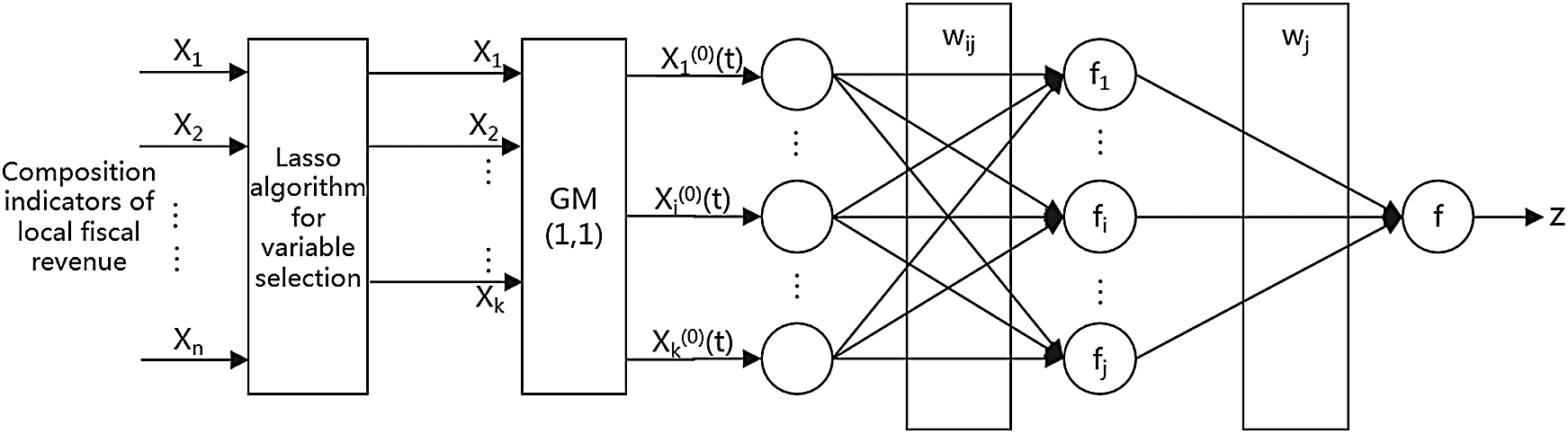
Figure 2: The proposed model

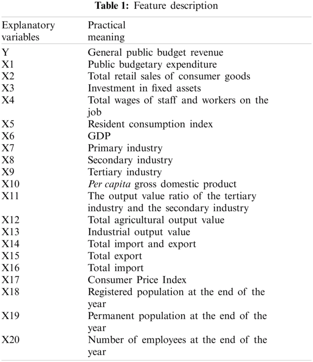
3.1 Data Acquisition and Variable Selection

The main factors affecting local fiscal revenue are: general public budget expenditure, total retail sales of consumer goods, fixed asset investment, total wages of employees, resident consumption index, regional GDP and other indicators. By consulting the local fiscal revenue structure analysis literature data, combined with the current economic situation of Hunan Province, we chose general public budget revenue as the explained variable, and 20 explanatory variables such as public budget expenditure, fixed asset investment, and so on [26–28]. These explanatory variables are shown in Tab. 1. We selected the latest data for 15 years from 2005 to 2019 for the experiment. The amount of data can not only reflect the changes in data, but also meet the small sample size required by the gray model. The selected fiscal revenue data sample size does not exceed 20, which is in line with the excellent feature of the gray system in predicting the small sample size. All data are from the "Hunan Provincial Statistical Yearbook 2020" (http://222.240.193.190/2020tjnj/indexch.htm).

3.2 Data Description and Statistics

We firstly carried out a comprehensive statistical description of the data and got a comprehensive grasp of the existing data. Usually the analysis of data statistics uses the maximum value, minimum value, average value, and standard deviation to make the overall description. We used python’s built-in functions to directly find these four quantities, and then used the Pandas library to convert the data to Dataframe type. The output is shown in Tab. 2.

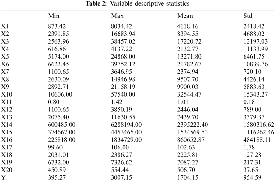
Combined with the original data and the statistical indicators in Tab. 2, it can be seen that the local budget revenue of Hunan Province has increased significantly and all the indicators have also increased comprehensively. The standard deviation of the explained variable Y is as high as 954.59, indicating that there is a great difference between the data of each year. Since 2010, the local budget income has grown substantially, which also indicates that Hunan has been developing rapidly in the recent ten years. Through the analysis of the explanatory variables X6, X7, X8, and X9, it can be seen that the GDP of Hunan Province has been rising steadily. In the ten years from 2005 to 2015, the secondary industry’s GDP accounted for the highest proportion and the growth rate was the fastest. This shows that Hunan Province has vigorously developed industry and introduced a large number of industrial production enterprises in the past decade. In 2016, the tertiary industry’s GDP began to surpass. The industrial structure of the entire Hunan Province has begun to gradually transform, and the service industry has slowly risen. Linking the variables X3 and X4, this shows that the living income of Hunan residents has increased and the living standards have been greatly improved, thus attracting more people to live and develop in Hunan, and increasing the values of the variables X18, X19, and X20.

3.3 Correlation Analysis

Correlation analysis is a statistical method used to describe the correlation between variables. Because the correlation is a non-deterministic relationship, it can be used to initially judge the degree of correlation between the dependent variable and the explanatory variable. The commonly used correlation analysis coefficients are Pearson correlation coefficient and Spearman rank correlation coefficient. The Pearson coefficient is used in the experiment. The formula of Pearson coefficient is as follows:

p=∑(X−X¯)(Y−Y¯)∑(X−X¯)2∑(Y−Y¯)2,−1≤p≤1 (19)

Based on the correlation coefficient p, the correlation degree could be obtained, which is shown in Tab. 3.

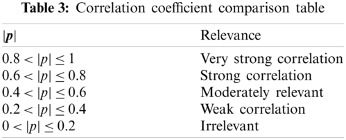
In order to show the degree of correlation more intuitively, we used a heat map to display the correlation coefficients of these 20 explanatory variables, as shown in Fig. 3.

It can be seen from the above Fig. 3 that the blue column represents the positive correlation between features, while the red column represents the negative correlation between features. The deeper the blue is, the stronger the correlation is, while the deeper the red is, the weaker the correlation is. Among them, the variables X11, X17, and X20 are relatively weak in correlation with the other explanatory variables, so they will be eliminated in the later feature selection.

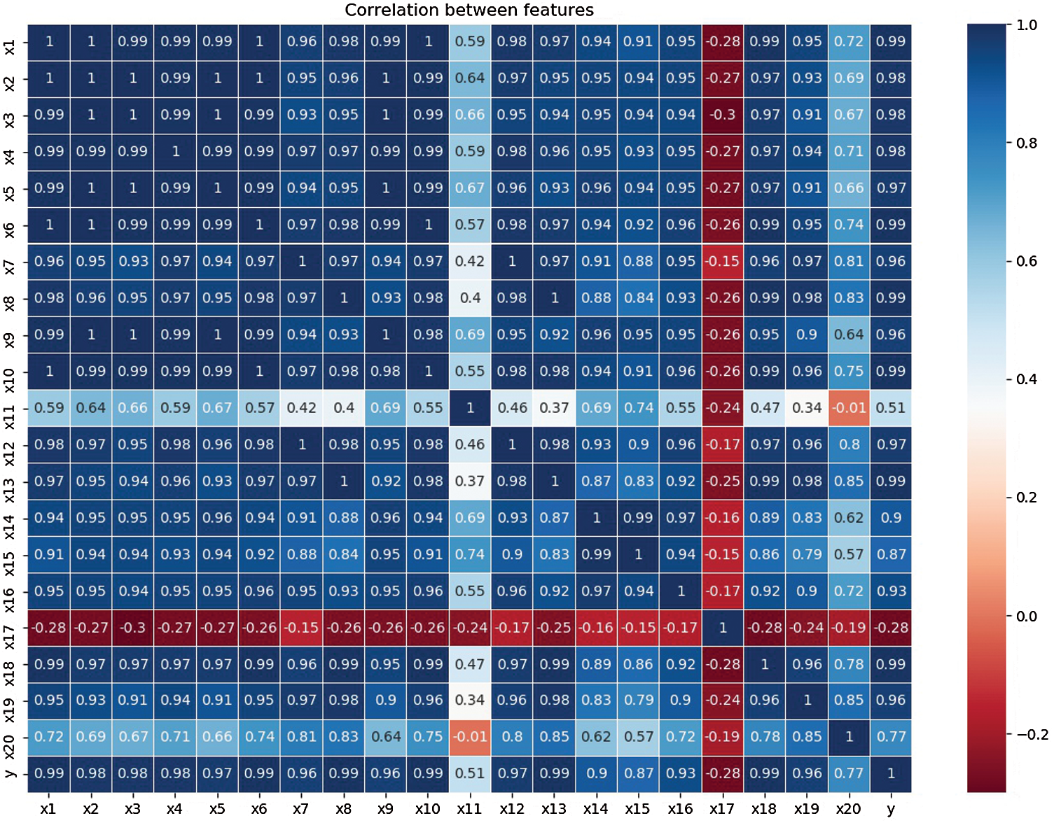
Figure 3: The heat map of Pearson coefficient for all variables

3.4 Feature Selection and Dimensionality Reduction

Since a total of 20 explanatory variables are selected, the sample data is relatively complicated and the features are not obvious, so the Lasso algorithm is used to achieve dimensionality reduction, and select the most important features. By calling python's SKLEARN library and executing the Lasso algorithm, the results obtained are shown in Tab. 4.

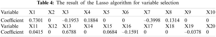
It can be clearly seen from Tab. 4 that the variables X1, X3, X4, X7, X8, X11, X13, X15, X16, and X19 will be retained after dimensionality reduction with Lasso algorithm, and other explanatory variables X2, X5, X6, X9, X10, X12, X14, X17, X18, and X20 will be removed because their coefficient is 0, which is regarded as irrelevant.

4  Data Forecasting and Result Analysis

4.1 Grey Model Predicting General Public Budget Revenue

After screening in the previous section, 10 explanatory variables are retained from the original 20 explanatory variables. By using the gray model, these 10 variables are used one by one to predict short-term data in order to obtain the values for 2020 and 2021. We took the compiled GM(1,1) program as a class object and directly imported it into the main program, then predicted the data of 10 explanatory variables. It is necessary to test whether the variable data is applicable to the gray prediction model before predicting, and the smooth ratio is an indicator specifically used to measure the applicability.

In this paper, the explanatory variable X7 was selected to show the prediction effect of the grey prediction model. Firstly, data applicability test was carried out. When the original data with smoothness less than 0.5 accounts for more than 60%, the test indicates that the data is suitable for the grey prediction model. The smoothness of the original data in each year is shown in Fig. 4. It can be seen that the proportion of less than 0.5 reaches 85.7%, so the data could be predicted by the gray model.

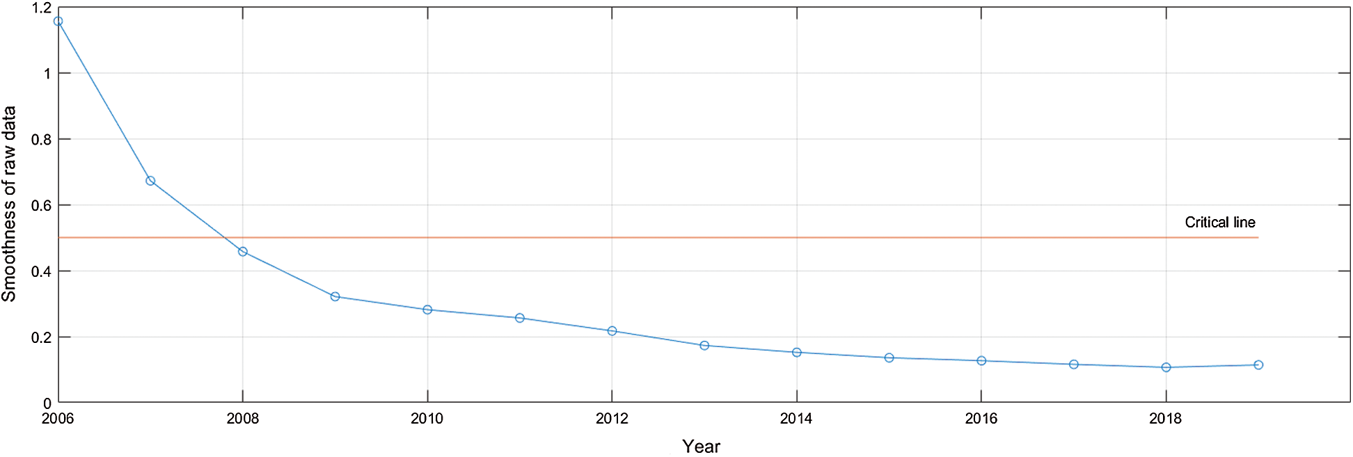
Figure 4: The smooth ratio of the explanatory variable X7

By bring the data of X7 into the GM(1,1) model, we used the original data for fitting and prediction. The result is shown in Fig. 5. It can be seen from Fig. 5 that there is a small error between the fitted data and the original data. The forecast result show an upward trend, which indicates that the total value of the primary industry in Hunan Province will increase steadily in 2020 and 2021. However, the effect of the graph cannot alone determine the quality of the fitting and prediction. There are scientific methods to measure the quality of model prediction and fitting results.

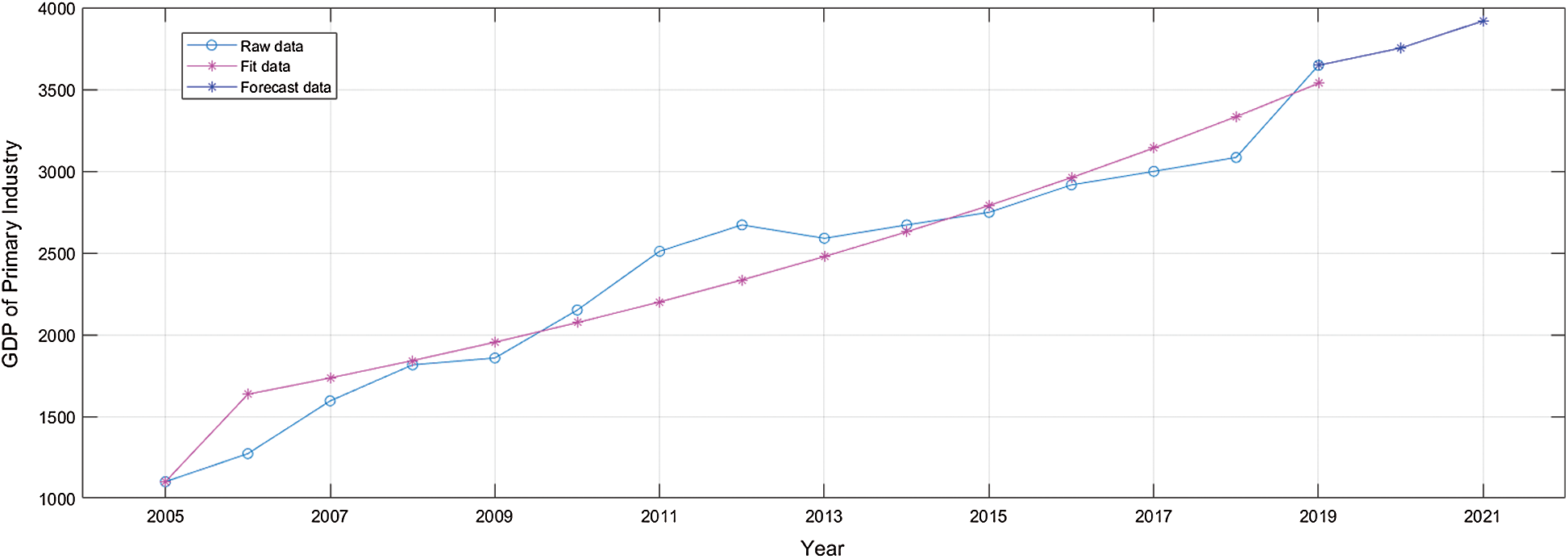
Figure 5: The original data, fitting data and prediction data of the explanatory variable X7

There are usually two indicators used to describe the degree of data fitting results: the relative residuals and the grade ratio deviation. When the relative residuals is less than 0.2 and the order ratio deviation is less than 0.15, the model fitting effect will be very good. We calculated the relative residuals and the grade ratio deviations of the X7 variable for each year, as shown in Fig. 6. It can be clearly seen from Fig. 6 that the relative residuals and the grade ratio deviations of the GM(1,1) model’s fitting data pass the test very well.

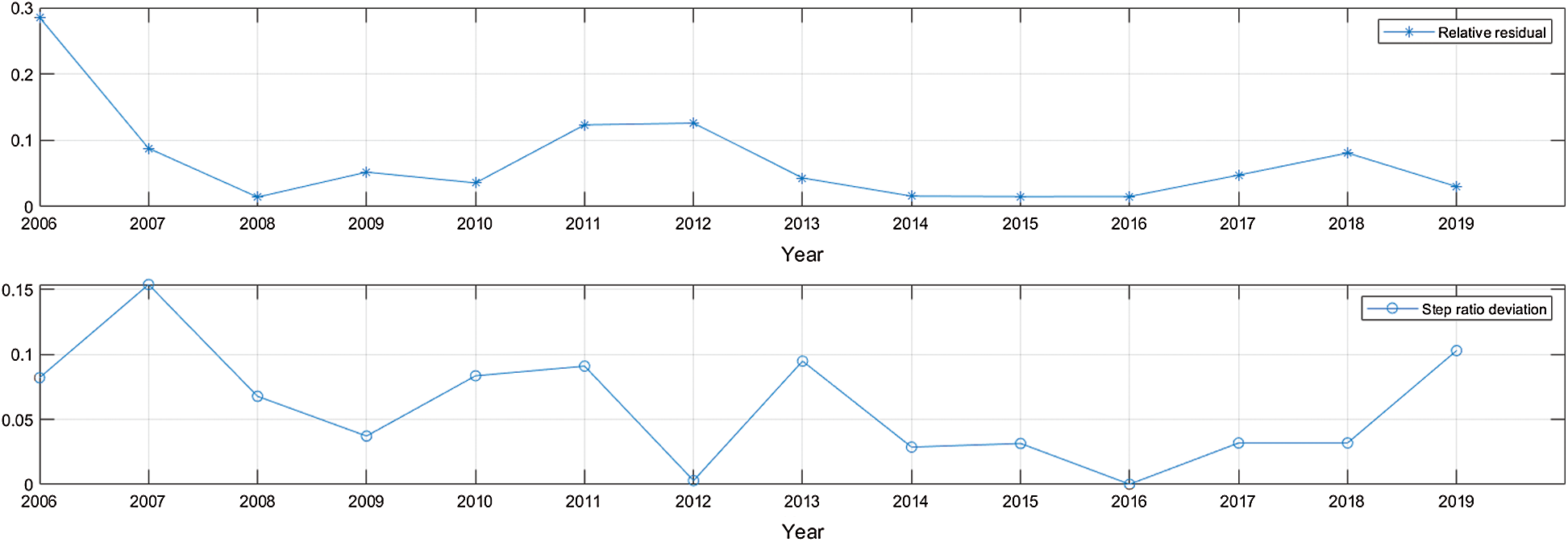
Figure 6: The relative residuals and step ratio deviation of the explanatory variable X7

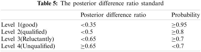
The posterior difference ratio is usually used to verify the quality of the predicted data. It has a set of test standards, as shown in Tab. 5. For the forecasting data of 2020 and 2021, the posterior difference ratio of the X7 is 0.27032, which meets the first-level accuracy standard.

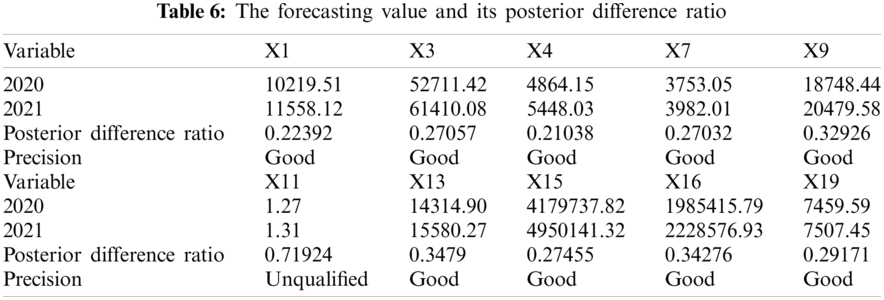
By using the GM(1,1) model, all the explanatory variables were predicted for 2020 and 2021, and the posterior difference ratio was used to test whether the prediction is good or bad. The results are shown in Tab. 6. It can be seen from the table that except for the variable X11, the other prediction accuracy is very good, which also proves that the gray prediction model has a very good prediction effect for short-term time series. In view of the predicting effect of the variable X11 is not good, which may affect the use of neural network to predict the fiscal revenue in the later period, so the variable X11 is artificially removed in the experiment.

Since the above experiments proved the feasibility and the accuracy of the GM(1,1) model to predict the shorter time series data, we directly used the GM(1,1) model to predict the variable Y (financial revenue), and the result is shown in Fig. 7. It can be seen from the figure that the data fitting has achieved good results, but the forecasting effect is obviously faster than the growth trend in previous years. Through analysis, we find that the fiscal revenue is affected by multiple variables, but the GM(1,1) model only predicts the future trend based on the data of current variables, without considering other influencing factors, so the forecasting results are inaccurate. So we decide to use the neural networks to make predictions.

4.2 Neural Network Predicting General Public Budget Revenue

By using the GM(1,1) model, we get the predicted values of 9 explanatory variables X1, X3, X4, X7, X8, X13, X15, X16, and X19, and then we can use the neural network to predict the financial revenue. The neural network model needs to set the number of layers of the network in advance, and the hidden layer of the BP neural network model usually does not exceed two layers. The sample size here is not large, so only two hidden layers are used. The setting of the number of neurons in the hidden layer is also skillful. If the number of nodes in the hidden layer is too small, the network cannot have the necessary learning and information processing capabilities. On the contrary, if it is too much, it will not only greatly increase the complexity of the network structure, but also slow down the learning speed. The Kolmogorov method [29] is most commonly used when setting the number of neurons in the hidden layer, and it is set to 19.

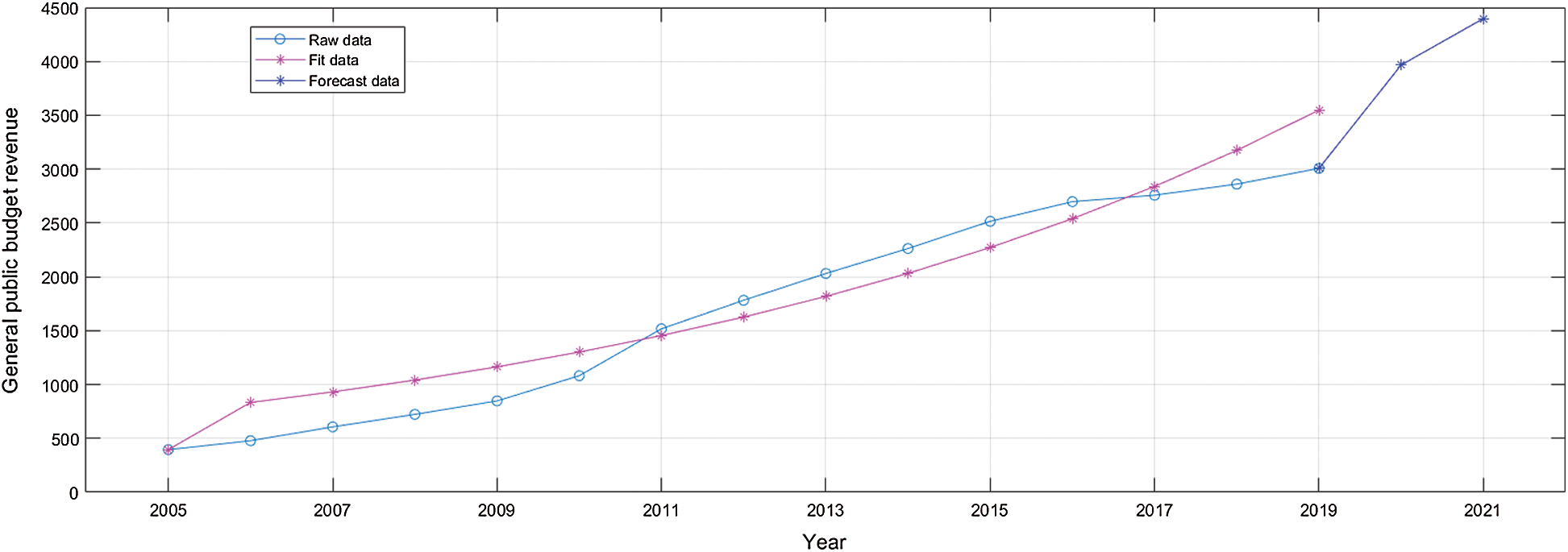
Figure 7: The GM(1,1) model predicting the financial revenue

Because the neural network model is particularly sensitive to data, if there is a big difference in the magnitude of the data, the accuracy of the trained model will be very poor. Therefore, it is necessary to ensure that each of the 9 explanatory variables is at the same magnitude before the formal training begins. The z-score method is used for standardization.

New datas=Raw datas−MeanStandard deviation (20)

There is a very useful Keras library in Python, which is an open source advanced deep learning library that can run on TensorFlow or Theano. We used the Keras library to build a 3-layer BP neural network, and the ReLU function was used as the activation function. When Keras library is used to build BP neural network, there is a very key parameter- BATCH_SIZE, which represents the number of samples used in one iteration of the algorithm. When the parameter is too large, although it will reduce the number of iterations, it will make the gradient descent effect worse, which makes the model effect bad. When the parameter is too small, the correction direction will be corrected by the gradient direction of the respective sample, which is difficult to converge. The BATCH_SIZE parameter in the experiment was set to 7.

After training the neural network model, we used the model.predict() function to predict the value of the financial revenue in 2020 and 2021. The result is shown in Fig. 8. It can be clearly seen from the figure that the fiscal revenue in 2020 and 2021 have a relatively stable upward trend. Compared with the prediction results of using the GM(1,1) model alone in the previous section, the upward trend of the prediction results of using the neural network is more gentle and more in line with the growth law of previous years. This is because the neural network model combines multiple influences, so it is obviously more convincing than the univariate prediction of the GM(1,1) model.

Figure 8: Comparison of the original data and the forecast data

The prediction result of the neural network is better, but compared with the actual fiscal revenue data released by Hunan Red Net, the predicted value in 2020 is much higher than the actual value. The actual fiscal revenue in 2020 is 300.87 billion yuan with a growth rate of 0.1%, and the forecast fiscal revenue in 2020 is 347.2056 billion yuan with a growth rate of 15.4%. The actual average growth rate from 2005 to 2019 was 14.48%. The growth rate predicted by the neural network is consistent with the growth rate of the previous 15 years. The reason for the low actual fiscal revenue is the outbreak of the new crown pneumonia epidemic in early 2020. Hunan Province has introduced tax and fee reduction policies in response to the new crown epidemic. Affected by both tax and fee reduction policies and the epidemic, Hunan's fiscal revenue continued to decline, so the actual fiscal revenue was lower than expected.

5  Conclusions

In order to overcome the problem of poor prediction accuracy caused by a single model, this paper proposed a combined model based on GM (1, 1) and the neural network to predict fiscal revenue. In order to verify the prediction effect of the model, we analyzed the fiscal statistical data of the 2020 Hunan Statistical Yearbook from 2005 to 2019, and selected 20 main indicators that affect the fiscal revenue as explanatory variables. Secondly, we used the Lasso algorithm to reduce dimensionality to select the most important 10 variables from these 20 explanatory variables. Thirdly, we chose the gray prediction model GM(1,1) to predict each single variable, and used the predicted value as the input of the neural network. Finally, we applied the BP neural network to forecast the fiscal revenue. Experimental results show that this combined model has a better prediction effect. In the next work, we will try other variable selection algorithms, such as the principal component analysis method, which is used to process the variables in the early stage, and then predict combined with the RBF neural network to achieve better prediction results.

Acknowledgement: The authors would like to appreciate all anonymous reviewers for their insightful comments and constructive suggestions to polish this paper in high quality.

Funding Statement: This research was funded by the National Natural Science Foundation of China (No.61304208), Scientific Research Fund of Hunan Province Education Department (18C0003), Research project on teaching reform in colleges and universities of Hunan Province Education Department (20190147), Changsha City Science and Technology Plan Program (K1501013-11), Hunan Normal University University-Industry Cooperation. This work is implemented at the 2011 Collaborative Innovation Center for Development and Utilization of Finance and Economics Big Data Property, Universities of Hunan Province, Open project, grant number 20181901CRP04.

Conflicts of Interest: The authors declare that they have no conflicts of interest to report regarding the present study.

References

 1.  Y. W. Wu and J. Q. Mao, “Local fiscal revenue under the tax-sharing system—An empirical analysis taking Shanxi province as an example,” Research on Financial and Economic Issues, vol. 3, pp. 100–104, 2009. [Google Scholar]

 2.  H. Akaike, “A new look at the statistical model identification,” IEEE Transactions on Automatic Control, vol. 19, no. 6, pp. 716–723, 1974. [Google Scholar]

 3.  R. Tibshirani, “Regression shrinkage and selection via the lasso,” Journal of the Royal Statistical Society Series B (Methodological), vol. 58, no. 1, pp. 267–288, 1996. [Google Scholar]

 4.  I. E. Frank and J. H. Friedman, “A statistical view of some chemometrics regression tools,” Technometrics, vol. 35, no. 2, pp. 109–135, 1993. [Google Scholar]

 5.  L. Breiman, “Better subset regression using the nonnegative garrote,” Technometrics, vol. 37, no. 4, pp. 373–384, 1995. [Google Scholar]

 6.  M. Li, “Influencing factor of financial revenue and forecast of financial revenue in Gansu province,” M.S. Thesis, Department of Mathematics, Shandong University, Shandong, China, 2016. [Google Scholar]

 7.  S. F. Liu, Y. G. Dang, Z. G. Fang and N. M. Xie, “The concept and basic principles of grey system GM(1,1) model,” in Grey System Theory and Application. Beijing, China: Science Press, pp. 1–28, 2010. [Google Scholar]

 8.  Z. Peng, “National revenue forecast model based on data analysis,” M.S. Thesis, Department of Statistics, Beijing Institute of Technology, Beijing, China, 2016. [Google Scholar]

 9.  Z. X. Wang, Y. G. Dang, S. F. Liu and Z. W. Lian, “Solution of GM(1,1) power model and its properties,” System Engineering and Electronics, vol. 31, no. 10, pp. 2380–2383, 2009. [Google Scholar]

10. R. P. Yuan, J. D. Li and Z. Y. Tian, “Science park revenue forecast based on GM(1,1) residual model,” Mathematics in Practice and Theory, vol. 46, no. 18, pp. 109–114, 2016. [Google Scholar]

11. G. Sun, H. Lv, D. Wang, X. Fan, Y. Zuo et al., “Visualization analysis for business performance of Chinese listed companies based on Gephi,” Computers Materials & Continua, vol. 63, no. 2, pp. 959–977, 2020. [Google Scholar]

12. L. Xiang, G. Guo, Q. Li, C. Zhu, J. Chen et al., “Spam detection in reviews using LSTM-based multi-entity temporal features,” Intelligent Automation & Soft Computing, vol. 26, no. 6, pp. 1375–1390, 2020. [Google Scholar]

13. F. Chollet, “Xception: Deep learning with depthwise separable convolutions,” in 2017 IEEE Conf. on Computer Vision and Pattern Recognition (CVPRHonolulu, HI, pp. 1800–1807, 2017. [Google Scholar]

14. X. C. Luo, R. H. Shen, J. Hu, J. H. Deng, L. J. Hu et al., “A deep convolution neural network model for vehicle recognition and face recognition,” Procedia Computer Science, vol. 107, pp. 715–720, 2017. [Google Scholar]

15. F. Fang and L. He, “Fiscal revenue prediction about the ARMA-BP neural network combination model,” Journal of Mathematics, vol. 32, no. 3, pp. 709–713, 2015. [Google Scholar]

16. F. Jiang, T. Zhang and Y. L. Zhou, “Local fiscal revenue forecast based on Lasso-GRNN neural network model,” Statistics & Decision, vol. 34, no. 19, pp. 91–94, 2018. [Google Scholar]

17. T. Chen and X. H. Zhou, “Prediction model of deep sensor based on BP neural network,” Computer & Digital Engineering, vol. 47, no. 12, pp. 2978–2981, 2019. [Google Scholar]

18. S. Reid, R. Tibshirani and J. H. Friedman, “A study of error variance estimation in lasso regression,” Statistica Sinica, vol. 26, pp. 35–67, 2014. [Google Scholar]

19. Z. D. Xu and F. X. Liu, “Survey on gray GM(1,1) model,” Computer Science, vol. 43, no. 11, pp. 6–10, 2016. [Google Scholar]

20. S. F. Liu, B. Zeng, J. F. Liu and N. M. Xie, “Several basic models of GM(1,1) and their applicable bound,” Systems Engineering and Electronics, vol. 36, no. 3, pp. 501–508, 2014. [Google Scholar]

21. G. H. Yang, Y. Yan and H. Z. Yang, “Application of improved GM(1,1) grey prediction model,” Journal of Nanjing University of Science and Technology, vol. 44, no. 5, pp. 575–582, 2020. [Google Scholar]

22. D. E. Rumelhart, G. E. Hinton and R. J. Williams, “Learning representations by back-propagating errors,” Nature, vol. 323, no. 9, pp. 533–537, 1986. [Google Scholar]

23. S. W. Lee, “Optimisation of the cascade correlation algorithm to solve the two-spiral problem by using CosGauss and sigmoid activation functions,” International Journal of Intelligent Information and Database Systems, vol. 8, no. 2, pp. 97–116, 2014. [Google Scholar]

24. J. H. Liu, D. Y. Fan and R. L. Tian, “Neural network prediction model of rolling force based on ReLU activation function,” Forging & Stamping Technology, vol. 41, no. 10, pp. 162–165, 2016. [Google Scholar]

25. X. Glorot and Y. Bengio, “Understanding the difficulty of training deep feedforward neural networks,” in Proc. of the Thirteenth Int. Conf. on Artificial Intelligence and Statistics (PMLRChia Laguna Resort, Sardinia, Italy, pp. 249–256, 2010. [Google Scholar]

26. J. Chao, “The influencing factors of China's fiscal revenue and evaluation of forecast,” Sub National Fiscal Research, vol. 2, pp. 41–46, 2016. [Google Scholar]

27. Y. L. Wang and C. C. Liang, “An empirical study on the influencing factors of government fiscal transparency based on provincial panel data,” Commercial Research, vol. 12, pp. 58–64, 2015. [Google Scholar]

28. X. Ma and A. F. Zhao, “Factors of regional fiscal income differences—Based on the perspective of real estate business tax,” Public Finance Research, vol. 7, pp. 53–57, 2014. [Google Scholar]

29. R. Hecht-Nielsen, “Kolmogorov's mapping neural network existence theorem,” in Proc. of the 1st IEEE Int. Joint Conf. of Neural Networks, vol. 3, New York, NY, USA, pp. 11–14, 1987. [Google Scholar]

This work is licensed under a Creative Commons Attribution 4.0 International License, which permits unrestricted use, distribution, and reproduction in any medium, provided the original work is properly cited.