DOI:10.32604/cmc.2022.019071
| Computers, Materials & Continua DOI:10.32604/cmc.2022.019071 | |
| Article |
Model Identification and Control of Evapotranspiration for Irrigation Water Optimization
1Department of Exact Sciences, Normal Higher School of Bechar, 08000, Algeria
2Laboratory of Energetic in Arid Zones, Faculty of Technology, Tahri Mohammed University of Bechar, 08000, Algeria
3Department of Mathematics and Computer Science, Faculty of Exact Sciences, Tahri Mohammed University of Bechar, 08000, Algeria
4Algerian Institute for Research in Agronomy, Experimental Station of Adrar, 01000, Algeria
*Corresponding Author: Wafa Difallah. Email: wafadif@gmail.com
Received: 31 March 2021; Accepted: 12 May 2021
Abstract: Water conservation starts from rationalizing irrigation, as it is the largest consumer of this vital source. Following the critical and urgent nature of this issue, several works have been proposed. The idea of most researchers is to develop irrigation management systems to meet the water needs of plants with optimal use of this resource. In fact, irrigation water requirement is only the amount of water that must be applied to compensate the evapotranspiration loss. Penman-Monteith equation is the most common formula to evaluate reference evapotranspiration, but it requires many factors that cannot be available in many cases. This leads to a trend towards behavior model estimation. System identification with control is one of the most promising applications in this axis. The idea behind this proposal depends on three stages: First, the estimation of reference evapotranspiration (ET0) by a linear ARX model, where temperature, relative humidity, insolation duration and wind speed are used as inputs, and ET0 estimated by Penman-Monteith equation as output. The results show that the values estimated by this method were in good agreement with the measured data. The second part of this paper is to manage the quantity of water. For this purpose, two controllers are used for testing, lead-lag and PID. To adjust the first controller and optimize the choice of its parameters, Nelder-Mead algorithm is used. In the last part, a comparative study is done between the two used controllers.
Keywords: Evapotranspiration; water; identification; optimization; irrigation; control
The importance of water resource does not need to be proved. At first sight water seems to be the most abundant resource on earth, but in fact freshwater represents only 1% of all terrestrial water, and the remaining 99% are not available for human use. Algeria, like all African countries is largely affected by this water shortage, knowing that most of the country is a desert (87%) where rainfall is almost rare, and between 15 and 20 billion m3of water should be provided annually, reserving 70% for agriculture to achieve satisfactory food security. It is a titanic challenge when we know that we mobilize barely 5 billion cubic meters of water per year. In addition, the pressure on these resources will continue to grow, under the effects of population growth, urbanization and pollution.
The importance of water for plants is no longer to be demonstrated. Among all economic sectors, irrigation is the sector where water scarcity has the greatest impact. Currently it is the largest consumer; it is also the sector with the most adjustment possibilities. Although it is only a small part of the global water cycle, evapotranspiration (ET) ensures the transfer of water from the soil to the atmosphere and plays a crucial role in the terrestrial biosphere. For most landscapes, evapotranspiration is governed by the transpiration of plants that draw water from the soil with their roots and return it to the atmosphere through the stomata of their leaves [1].
Measuring ET is a valuable information for estimating water availability, plant absorption, spatial distribution, and variation over time [2,3]. It is also related to soil moisture and can serve as an indicator of water stress. From an agricultural point of view, its spatialized measurement is therefore an essential tool for the management of water resources and the optimization of irrigation on a territorial scale.
This introduction explains the existence of several works to estimate this factor. Since 1950, several formulas have been developed: Thornthwaite (1944) [4], Turc (1962) [5], Blanney-Criddle (1950) [6] and Penman-Monteith-FAO (1998) [7]. The use of these models requires the knowledge of certain climatic data such as, the maximum and minimum temperature of the air, the maximum and minimum relative humidity, which depends on the temperature, global solar radiation and wind speed [8].
Several comparative studies have been conducted to determine the best method for calculating evapotranspiration [8–15].
Generally, the Penman-Monteith method leads to a better approximation of evapotranspiration. However, the implementation of this method requires a high number of parameters that are not always available for a simple farmer. This criticism implies the need to find simple and less expensive models in terms of the number of parameters for estimating evapotranspiration. A method of calculating ET0 is proposed in [16]. The principle of this method is very simple and evapotranspiration calculation is based only on temperature. Similarly, in [17], the ET0 is derived solely from the temperature by the Hargreaves method, due to the unavailability of other parameters. Therefore, it does not include the sensitivity of other parameters affecting ET0, as does the Penman-Monteith method. However, the Hargreaves method can be considered as a quality technique in the calculation of evapotranspiration if the required Penman-Monteith variables are not all available.
Generalized models based on the wavelet neural network (WNN) have been developed to estimate the reference evapotranspiration (ET0) corresponding to the Hargreaves (HG) method for different agro-ecological regions: semi-arid, arid, subhumid, and humid in India. The input and output of the WNN models are respectively the daily climatic data (minimum and maximum air temperature) and the evapotranspiration values (estimated by the FAO-56 method of Penman-Monteith) grouped over a period of five years [18]. The three-temperature model (3 T model) is another proposal that could be used to estimate actual evapotranspiration (ET) and assess the quality of the environment [19]. The main parameters included are the air temperature, the surface temperature of the soil and the reference soil temperature.
In [20,21], a neural network model was developed to estimate reference evapotranspiration. This model guarantees a precision close to the formula of Penman Montheith, and with less parameters. For the same reason, the energy balance equation was used by Takakura et al. in [22] to measure evapotranspiration. Authors conclude that this method can be helpful to optimize the irrigation process.
Several models have been proposed, in which the purpose was to obtain the value of ET at a lower cost in order to determine the irrigation water requirements. The methods used for this purpose are very varied, with the use of different parameters (temperature, solar radiation, etc.).
In this paper, system identification with the autoregressive polynomial method with exogenous variables (ARX) is chosen to model the ET0, and the estimated results are compared to the measured values to test and validate the obtained model. In another step, lead lag and PID controllers are used to control the quantity of water for crops irrigation, and a comparative study is done.
2 Materials and Methods of Modeling
The experiment was carried out in 2014, in the national institute of agronomic research (INRAA) in the south west of Algeria, exactly in the region of Adrar (27° 49’ North latitude and 00°18 East longitude (see Fig. 1), with 276 m elevation above sea level).
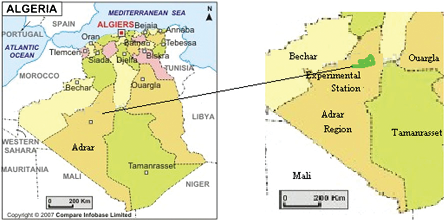
Figure 1: Location of the study area: INRAA [20]
In our study, we chose wheat crop, since Algeria is the third largest importer with 8.2 million tons after Egypt and Indonesia [23] (Fig. 2), hence the need to encourage the production of this type of cereal.
For the trials of the experimental station, it is a variety of durum wheat, commonly called “Shen-S”; it is semi-early and short-straw (85 cm), widely used under pivots.
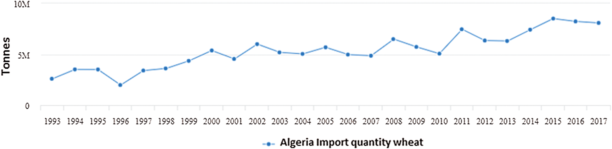
Figure 2: Imports of Wheat in Algeria 1993–2017 [24]
The temperature varies from 9°C in winter of 2014 to 44°C in summer (Fig. 3).
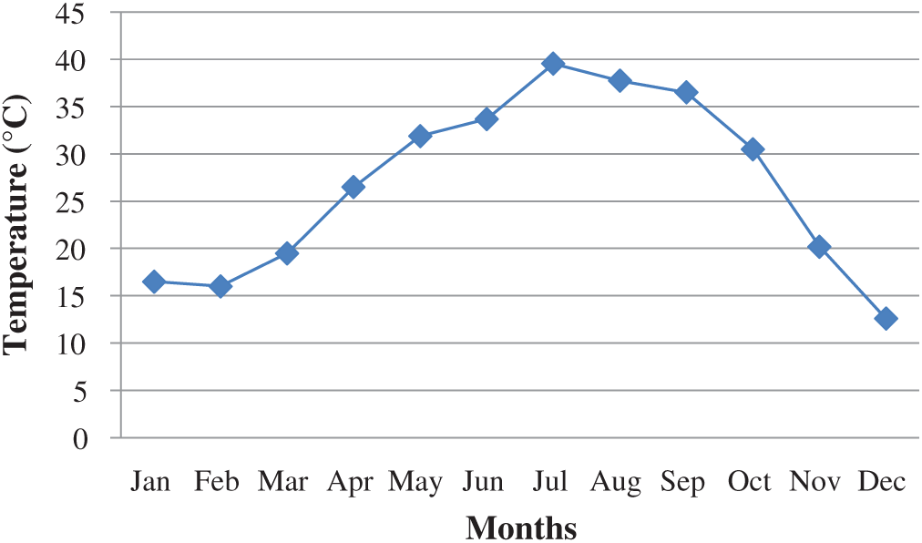
Figure 3: Evolution of the average temperature during the year
It is often less than 50%. It exceeds this value for four months of the year (January, February, November and December) (Fig. 4). During some very short periods (rainy days), it can approach 100%. Dew is a very rare event.
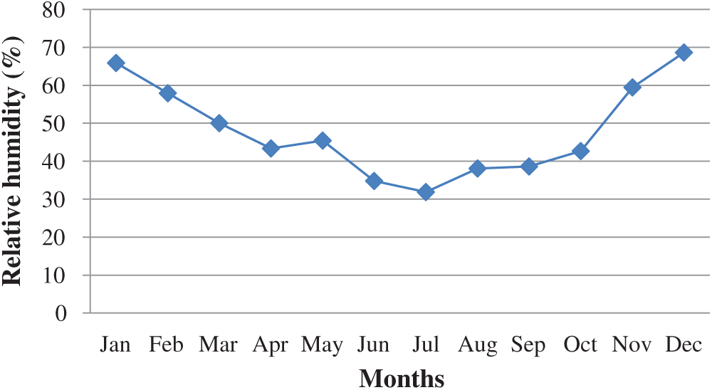
Figure 4: Evolution of the average relative humidity during the year
It blows almost constantly, the dominant direction is Northeast. Towards the west, it often blows in violent sandstorms carrying out a double action: erosion and transport and sedimentation. Although the average speed seems low, the instantaneous speed can be very high and can reach 100 Km/h (Fig. 5); it can cause significant damage to crops and protection systems (greenhouses, walls and windbreaks).
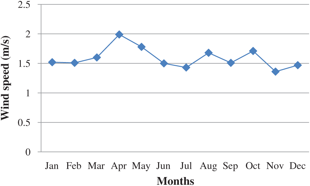
Figure 5: Evolution of the average wind speed during the year
The sunshine duration is often greater than 7 h a day. This indicates that the sky is clear most of the time (Fig. 6).
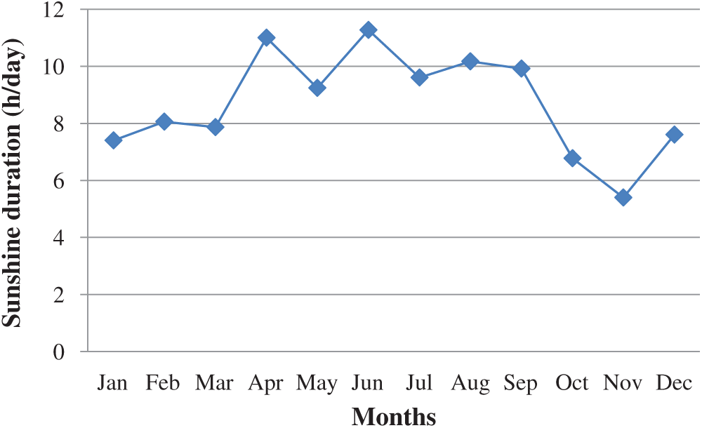
Figure 6: Evolution of the average sunshine duration during the year
The different climatic parameters are taken from the weather station located inside the experimental station (INRAA) of Adrar. These are temperature, relative humidity, wind speed, sunshine duration and evapotranspiration.
To calculate the reference evapotranspiration, the Penman-Montheith formula (Eq. (1)) proposed by Allen et al. (1998) is applied with the climatic parameters of July:
where Rn refers to the net radiation at the crop surface [MJ m−2 day−1], G refers to the soil heat flux density [MJ m−2 day−1], T refers to the mean of daily air temperature at 2 m height [°C], u2 designates the wind speed at 2 m height [m s−1], es refers to the saturation vapour pressure [kPa], ea refers to the actual vapor pressure [kPa], es-ea designates the saturation vapor pressure deficit [kPa], Δ refers to the slope vapor pressure curve [kPa °C−1], γ is the psychometric constant [kPa °C−1].
PT100 Thermometer, Hygrometer, Wind vane and anemometer and Pyranometer are respectively used to sense temperature, relative humidity, wind speed and sunshine duration (see Fig. 7).
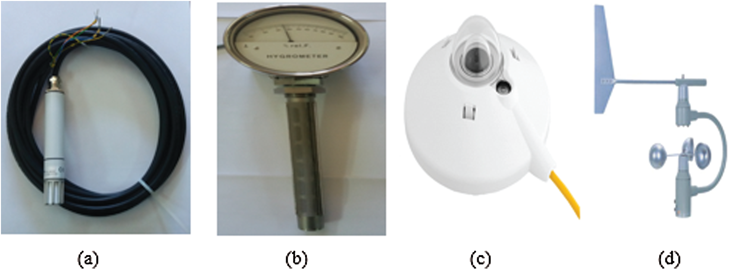
Figure 7: Different sensors used to collect data from the experimental site. (a- PT100 Thermometer, b-Hygrometer, c-Wind vane and anemometer, d-Pyranometer)
The values of ET0 are generally high. They are closely related to all other meteorological factors (Fig. 8).

Figure 8: ET0 estimated by Penman-Montheith formula
3 Identification of Reference Evapotranspiration
3.1 The Identification Process
To identify a real dynamic system (called object) is to characterize another system (called model) from the experimental knowledge of the inputs - outputs of the object [25]. The diagram below shows the inputs and outputs of the studied system (Fig. 9).
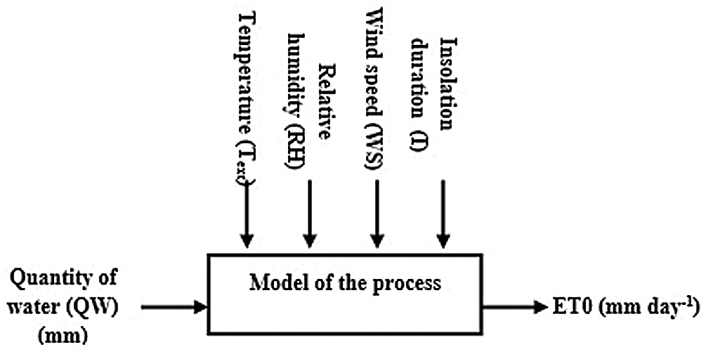
Figure 9: The input, output and disturbance signals of the studied system
The identification process is shown in the diagram in Fig. 11.
Initially the system is analyzed to understand its behavior and obtain a set of information that can help in the construction of the model. Depending on the knowledge of the system, an experimental plan is defined taking into account constraints and limitations. The experiment must be put into practice in such a way that the acquired data are obtained by exciting the whole range of frequencies to cover the widest possible range of the situations of its operation.
After collecting the data, following the analysis that has been done beforehand, a model structure is chosen (ARX, ARMAX, … etc.) [26]. The purpose of the model is to represent reality as accurately as possible. In this work, AutoRegressive models with eXogenous variables (ARX) are chosen. A diagram of an ARX model structure and its equation is illustrated in Fig. 10. The ARX model is a simple differential equation, which describes an input-output relationship. The input-output relationship is modeled by a B/A transfer function.
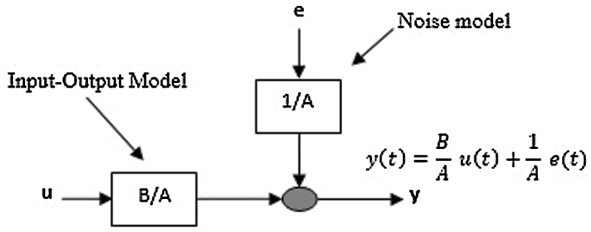
Figure 10: ARX model
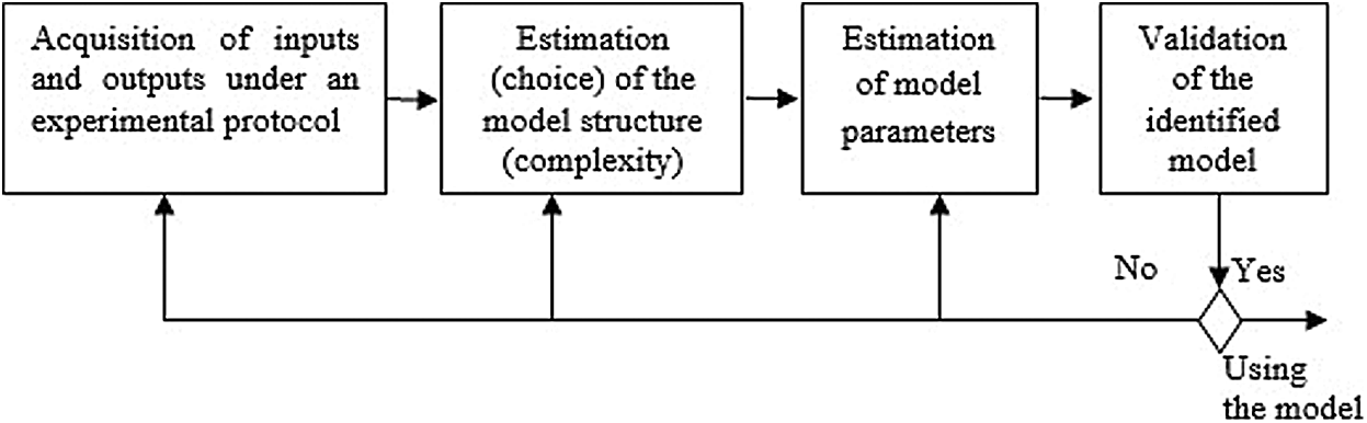
Figure 11: System identification procedure
The next step in the identification system procedure is to generate the model parameters. Matlab uses the least square algorithm to update the model parameters. In the presence of the model structure and the output data measured at the experimental site or generated from the process, the least squares algorithm estimates the parameters of the model. It must minimize the error between process or experimental outputs and outputs estimated by the model. If not, another model structure should be chosen [27].
To conclude on the relevance of the model, validation tests are carried out: a new data set is used and the behavior of the model is compared to reality.
The data with a simple time equal to 0, 01 s is separated into two subsets: 67% of the data is used for the estimation phase and 33% of the data is used for the validation phase. The large amount of data is used in the estimation phase to provide very satisfactory and adequate results.
3.3 Choice of the Model Structure
The ARX polynomial model chosen is written in the following form:
e(t) is a white noise.
3.4 Identification Principle of System Parameters
The parameters are identified according to the following diagram, i.e., by comparing the measured and calculated results and minimizing the errors between them with the Nelder-Mead optimization algorithm (Fig. 12).
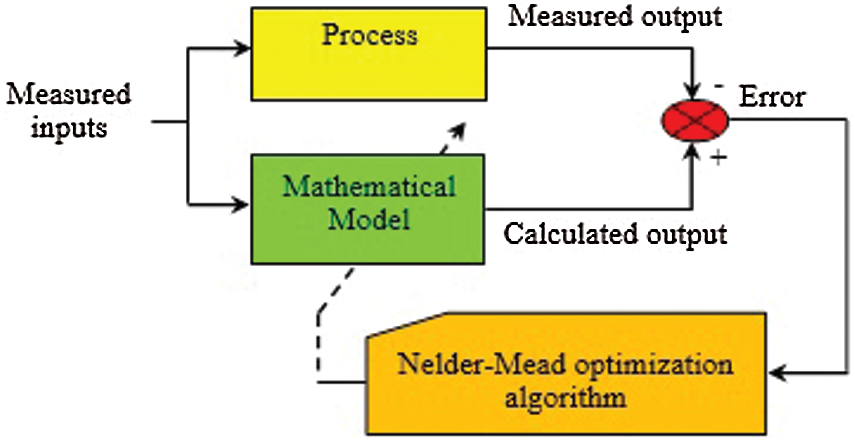
Figure 12: General schema of parameters identification
Fig. 13 represents system identification of evapotranspiration by the measurements collected at the experimental station.

Figure 13: Diagram of the ET0 model identification
The system studied is of the “multi-input, mono-output” type (Fig. 14).
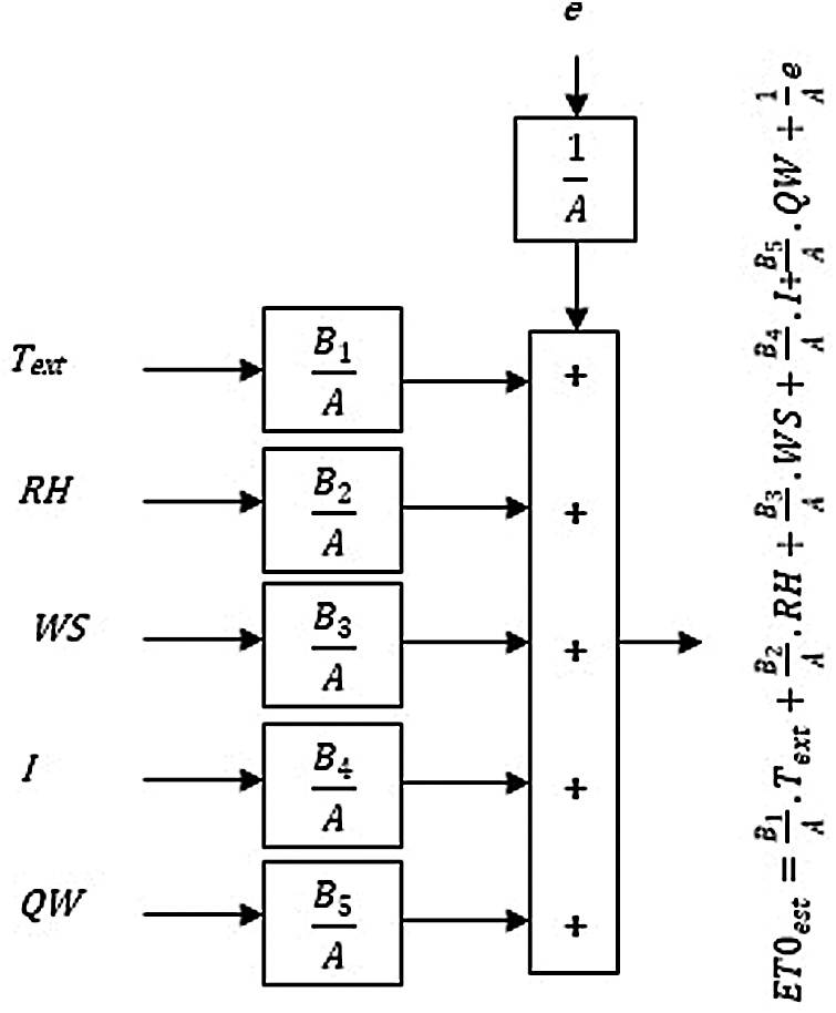
Figure 14: ARX model of the studied system
Model parameters estimated by hand tuning are presented in Tab. 1 below.
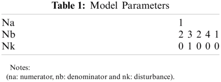
After system execution, the following discrete linear model is obtained:
In Polynomial Form
With
In transfer function form
Z: an operator.
In state space form
where the matrices a, b, c and d are:
To test the validity of the system, we compare the output of the identified model (ET0est) to the evapotranspiration calculated with Penman-Montheith formula using the measurements collected on site (ET0mes). The comparison with estimation and validation data is presented respectively in Figs. 15 and 16. As it is shown in the figures, there is a strong correlation between the computed evapotranspiration values and the values estimated by the identified ARX model.
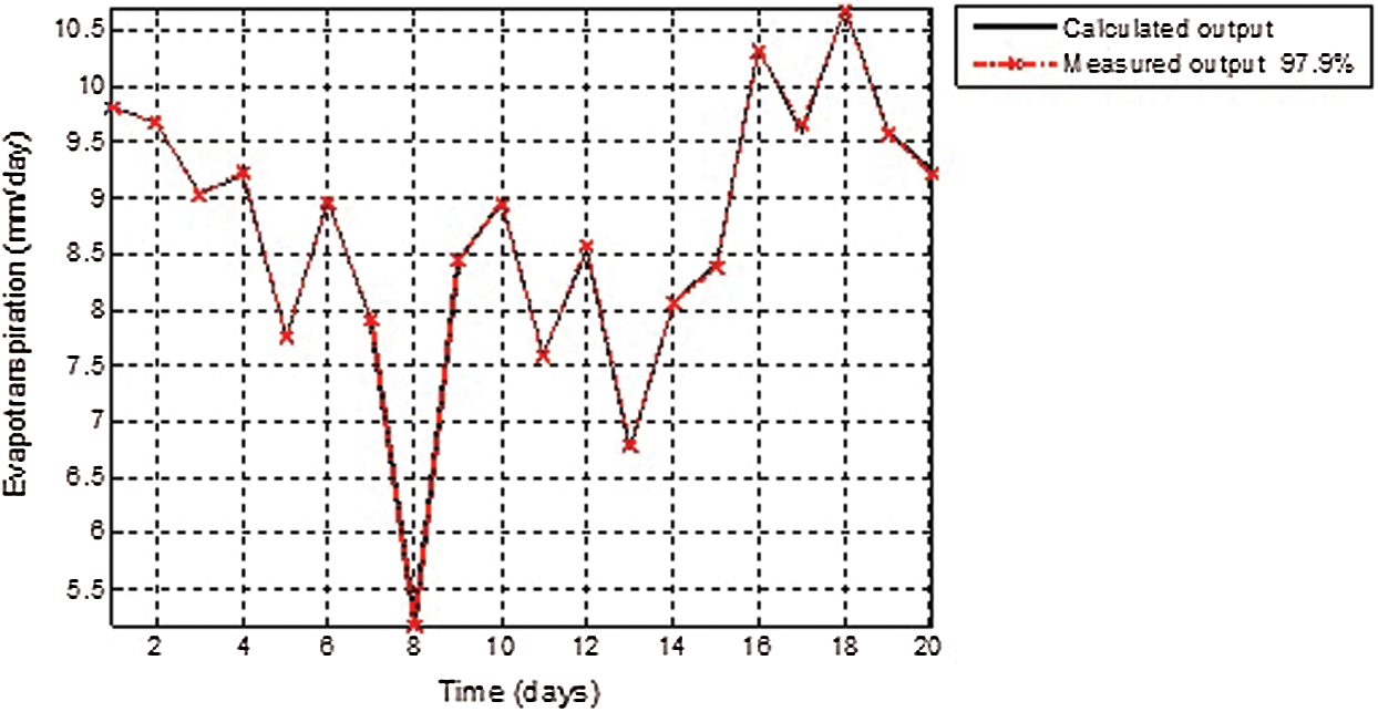
Figure 15: Evolution over time of ET0 estimation data
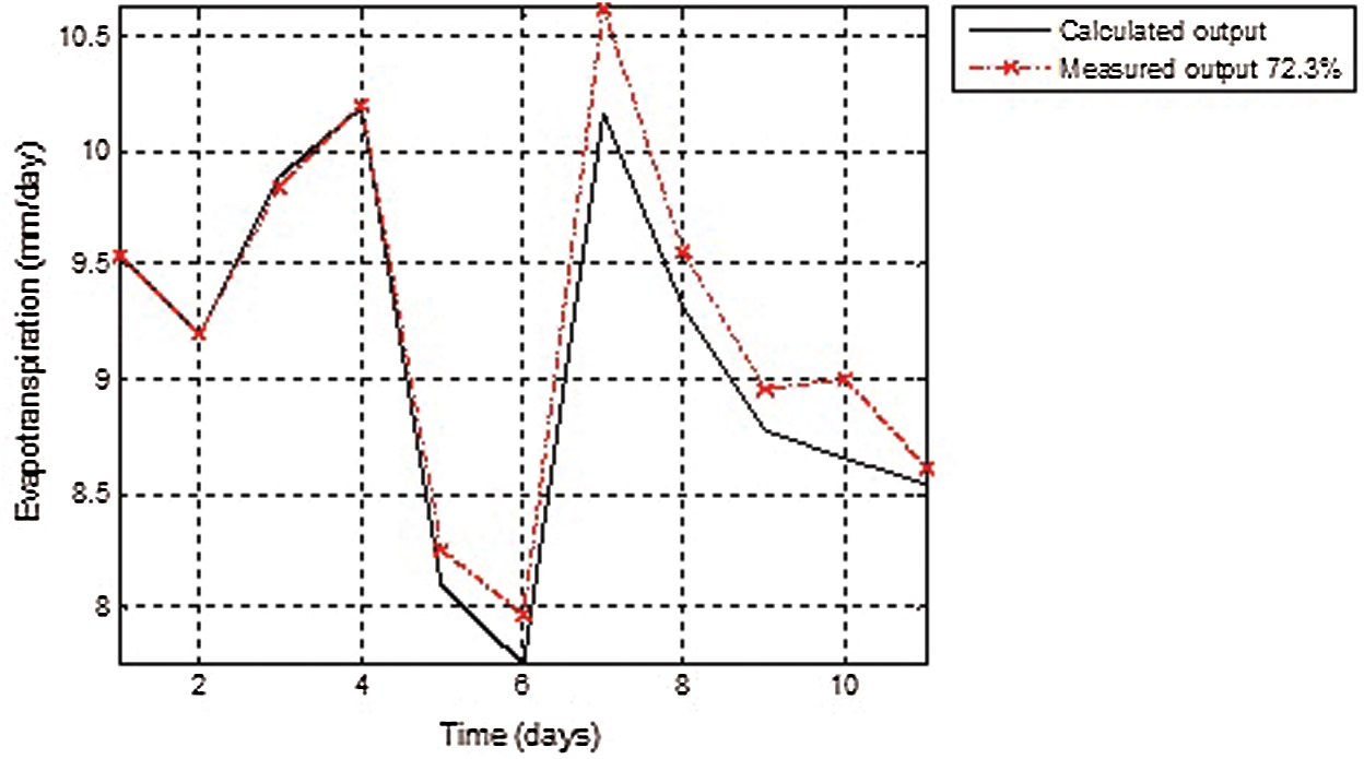
Figure 16: Evolution over time of ET0 validation data
4Control System
The second part in this paper is the control; an important step to determine the right amount of water for wheat irrigation. For this purpose, two most popular controllers are implemented: lead lag and PID, with ITAE (Integral Time Absolute Error index performance criterion) criterion optimized with Nelder-Mead algorithm, followed by a comparative study.
The control system design is illustrated in Fig. 17:

Figure 17: Control system design with ITAE criterion
The first chosen controller is lead lag compensator; widely used in linear and classical control system design [28,29] with the following general form:
The results, after optimization of zeros, poles and gain are shown in Tab. 2.
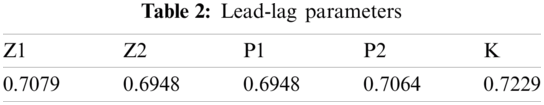
The simulation of the controlled system in Fig. 17 with lead-lag compensator demonstrates the feasibility of using this controller to define the needed water for crops irrigation (etolg). The latter will compensate the lack caused by evapotranspiration as shown in Fig. 18. This result illustrates that the evapotranspiration generated by lead-lag (etolg) is close to the desired evapotranspiration (etoref) as is indicated in Figs. 19 and 20.

Figure 18: Comparison between desired and simulated evapotranspiration (etoref-etolg)

Figure 19: Evolution of QW signal control generated by Lead-lag
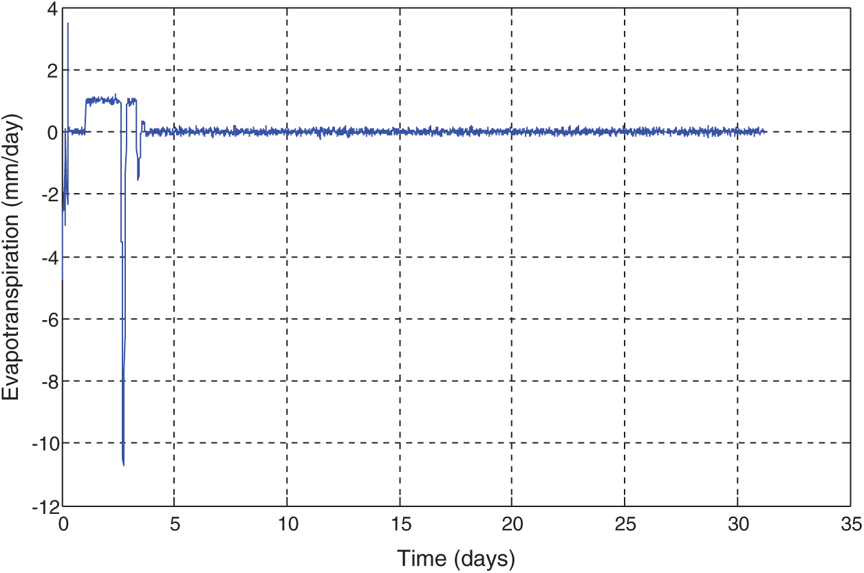
Figure 20: Difference between desired and simulated evapotranspiration (etoref-etolg)
The second chosen controller is the PID, well known with three terms controller. Each term constitutes a controller type in itself: proportional, integral, and derivative controller which depend respectively on the current error, the accumulation of past error, and the prediction of future error [30]. The PID is the collection of these three controllers, knowing that is possible to have two terms controller such as P, PI and PD controllers.
These terms represent the tuning parameters of the general PID controller given by:
With filtered derivative term:
In this system, hand-tuning method is used and the adjusted parameters are given in Tab. 3.
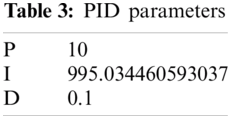
After replacing led-lag by PID controller in the system, it can be say that there is a good agreement between desired evapotranspiration and the quantity of water generated by PID. This is obviously confirmed in Figs. 21–23 where the error signal is almost null.

Figure 21: Comparison between desired and simulated evapotranspiration (etoref-etopid)
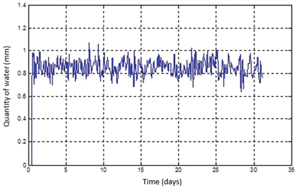
Figure 22: Evolution of QW signal control generated by PID

Figure 23: Difference between desired and simulated evapotranspiration (etoref-etopid)
As is shown in Fig. 17, after system identification, the controllers are tested with the use of a saturation block to guarantee that the system respects the physical conditions, and the results are shown in Fig. 24 below.

Figure 24: Comparative analysis of evapotranspiration evolution using PID and lead-lag controllers
Fig. 24 shows the comparative analysis of evapotranspiration variation using PID and lead-lag controllers. The two different controllers are implemented using MATLAB software. According to the simulation results, PID controller shows relatively better results than the lead lag controller.
Generally, the control system with the both controllers: PID and lead lag show encouraging results for the application of the estimated ET0 in real time to optimize the irrigation water use.
To identify a physical system is to characterize another system (called a model), based on the experimental knowledge of the inputs and outputs so as to obtain an identity of the behavior.
First, it is a question of collecting data, then choosing a structure of the model, an adjustment criterion and in the end retaining the best model. It is likely that the first model obtained does not achieve the desired level of precision, it will then be necessary to go back and review the different stages of the procedure.
In this study, a behavior model of reference evapotranspiration is identified using the ARX polynomial method.
This model is very close to the real system of Penman Montheith (97.9%), it is a great support for farmers to meet the water needs of crops with a few parameters.
As a second step, the obtained model is adjusted by a controller. For this purpose, two types of controllers are used and a comparative study is done to define which one provides the best results.
In this application, and as is well known in control system engineering, the PID controller remains the best, even though the results of the lead lag controller are also good and sometimes identical to the PID results as shown in Fig. 24.
In future studies, the aim will be to invest both controllers to obtain a more accurate system based on taking benefits of the two controllers and thus ensure a precise determination of plants water needs.
Funding Statement: The authors received no specific funding for this study.
Conflicts of Interest: The authors declare that they have no conflicts of interest to report regarding the present study.
1. L. Oudin, “Recherche d'un modèle d’évapotranspiration potentielle pertinent comme entrée d'un modèle pluie-débit global” Comparison of different methods of measuring the evapotranspiration of a rain-fed wheat crop, [In Frensh.], Ph.D. dissertation, ENGREF (AgroParisTech2004. [Google Scholar]
2. G. Bigeard, “Estimation spatialisée de l’évapotranspiration à l'aide de données infra-rouge thermique multi-résolutions” Spatialized estimation of evapotranspiration using multi-resolution thermal infrared data, [In Frensh], Ph.D. dissertation, Toulouse III University Paul Sabatier, France, 2017. [Google Scholar]
3. K. Djaman, H. Tabari, A. B. Balde, L. Diop, K. Futakuchi et al., “Analyses, calibration and validation of evapotranspiration models to predict grass-reference evapotranspiration in the Senegal river delta,” Journal of Hydrology: Regional Studies, vol. 8, pp. 82–94, 2016. [Google Scholar]
4. C. W. Thornthwaite, “Report of the committee on transpiration and evaporation,” Transaction of the American Geophysical Union, vol. 25, no. 5, pp. 683–693, 1944. [Google Scholar]
5. L. Turc, “Évaluation des besoins en eau d'irrigation, évapotranspiration potentielle,” Assessment of irrigation water requirements, potential evapotranspiration. [In frensh.],” Annales Agronomiques INRA, vol. 12, no. 1, pp. 13–50, 1961. [Google Scholar]
6. H. F. Blaney and W. D. Criddle, Determining Water Requirement in Irrigated Areas from Climatological Data, Washington, D.C, USA, Soil Conservation Service Technical Publication, vol. 96, pp. 1–48, 1950. [Google Scholar]
7. R. G. Allen, L. S. Pereira, D. Raes and M. Smith, Crop Evapotranspiration-Guidelines for Computing Crop Water Requirements, Rome, Italy, Food and Agriculture Organization, 1998. [Online]. Available: http://www.fao.org/tempref/SD/Reserved/Agromet/PET/FAO_Irrigation_Drainage_Paper_56.pdf. [Google Scholar]
8. F. Bouteldjaoui, M. Bessenasse and A. Guendouz, “Etude comparative des différentes méthodes d'estimation de l'évapotranspiration en zone semi-aride (cas de la région de djelfa),” Comparative study of the different methods for estimating evapotranspiration in semi-arid zones (case of the Djelfa region). [In Frensh.], Nature & Technologie, vol. 7, pp. 109–116, 2012. [Google Scholar]
9. C. A. Rim, “Comparison of approaches for evapotranspiration estimation,” KSCE Journal of Civil Engineering, vol. 4, pp. 47–52, 2000. [Google Scholar]
10. B. O. Delarozière, “Utilisation Comparée des Formules de Thornthwaite, Turc Mensuelle, Turc Annuelle et Penman, Pour le Calcul de L'évapotranspiration Réelle Moyenne-Application au Territoire Français,” Comparative use of Thornthwaite monthly Turc, annual Turc and Penman formulas, for the calculation of the average real evapotranspiration-Application to the French territory. [In Frensh.], Orleans, France, Frensh Geological Survey, pp. 1–19, 1971. [Online]. Available: http://infoterre.brgm.fr/rapports/71-SGN-173-HYD.pdf. [Google Scholar]
11. J. M. Peterschmitt and N. Katerji, “Comparaison de différentes méthodes de mesure de l’évapotranspiration d'une culture de blé non irriguée,” Comparison of different methods of measuring the evapotranspiration of a non-irrigated wheat crop. [In Frensh.], Agronomie, EDP Sciences, vol. 9, no. 2, pp. 197–205, 1989. [Google Scholar]
12. L. Zhao, J. Xia, C. Y. Xu, Z. Wang and L. Sobkowiak, “Evapotranspiration estimation methods in hydrological models,” Journal of Geographical Sciences, vol. 23, no. 2, pp. 359–369, 2013. [Google Scholar]
13. L. Jianbiao, S. Ge, S. G. McNulty and A. Devendra, “A comparison of six potential evapotranspiration methods for regional use in the southeastern United States,” Journal of the American Water Resources Association, vol. 41, no. 3, pp. 621–633, 2005. [Google Scholar]
14. J. Z. Drexler, R. L. Snyder, D. Spano and K. Tha Paw U, “A review of models and micrometeorological methods used to estimate wetland evapotranspiration,” Hydrological Processes, vol. 18, pp. 2071–2101, 2004. [Google Scholar]
15. A. Raza, M. Shoaib, M. A. Faiz, F. Baig, M. M. Khan et al., “Comparative assessment of reference evapotranspiration estimation using conventional method and machine learning algorithms in four climatic regions,” Pure and Applied Geophysics, vol. 177, pp. 4479–4508, 2020. [Google Scholar]
16. C. Riou, “Une formule empirique simple pour estimer l'évapotranspiration potentielle moyenne en tunisie,” A simple empirical formula to estimate the average potential evapotranspiration in Tunisia. [In Frensh.], Hydrol, vol. 17, no. 2, pp. 129–137, 1980. [Google Scholar]
17. S. Kundu, D. Khare and A. Mondal, “Future changes in rainfall, temperature and reference evapotranspiration in the central India by least square support vector machine,” Geoscience Frontiers, vol. 8, no. 3, pp. 583–596, 2017. [Google Scholar]
18. S. Adamala, “Temperature based generalized wavelet-neural network models to estimate evapotranspiration in India,” Information Processing in Agriculture, vol. 5, pp. 1–7, 2017. [Google Scholar]
19. Y. J. Xiong, G. Y. Qiu, J. Yin, S. H. Zhao, X. O. Wu et al., “Estimation of daily evapotranspiration by three-temperatures model at large catchment scale,” The International Archives of the Photogrammetry, Remote Sensing and Spatial Information Sciences, vol. 37, pp. 767–774, 2008. [Google Scholar]
20. A. Laaboudi, B. Mouhouche and B. Draoui, “Neural network approach to reference evapotranspiration modelling from limited climatic data in arid regions,” International Journal of Biometeorology, vol. 56, pp. 831–841, 2011. [Google Scholar]
21. A. Laaboudi, B. Mouhouche and B. Draoui, “Conceptual reference evapotranspiration models for different time steps,” Journal of Petroleum & Environmental Biotechnology, vol. 3, no. 4, pp. 1–8, 2012. [Google Scholar]
22. T. Takakura, C. Kubota, S. Sase, M. Hayashi, M. Ishii et al., “Measurement of evapotranspiration rate in a singlespan greenhouse using the energy-balance equation,” Biosystems Engineering, vol. 102, no. 3, pp. 298–304, 2009. [Google Scholar]
23. FAOSTAT, “Top 10 country importers, import quantity of wheat,” 2017. [Online]. Available: http://www.fao.org/faostat/en/#rankings/countries_by_commodity_imports. [Google Scholar]
24. FAOSTAT, “Crops and livestock products,” 2018. [Online]. Available: http://www.fao.org/faostat/en/#data/TP/visualize. [Google Scholar]
25. A. C. CemSay and S. Kuru, “Qualitative system identification: Deriving structure from behavior,” Artificial Intelligence, vol. 83, no. 1, pp. 75–141, 1996. [Google Scholar]
26. R. Liacu, “Identification de systèmes linéaires à paramètres variant (LPV) - Différentes approches et mises en œuvre” Identification of Linear Variant Parameter Systems (LPV) - Different approaches and implementations. [In Frensh.], Ph.D. dissertation, Doctoral school of sciences and information technologies, Telecommunications and Systems, France, 2014. [Google Scholar]
27. N. Rohrseitz and N. S. Fry, “Behavioural system identification of visual flight speed control in drosophila melanogaster,” Journal of the Royal Society, Interface, vol. 8, pp. 171–185, 2011. [Google Scholar]
28. Z. K. Jadoon, S. Shakeel, A. Saleem, A. Khaqan, S. Shuja et al., “A comparative analysis of PID, lead, Lag, lead-lag, and cascaded lead controllers for a drug infusion system,” Journal of Healthcare Engineering, vol. 2017, pp. 1–13, 2017. [Google Scholar]
29. F. Y. Wang, “The exact and unique solution for phase-lead and phase-lag compensation,” IEEE Transactions on Education, vol. 46, no. 2, pp. 258–262, 2003. [Google Scholar]
30. S. N. Norman, “A history of control systems,” in Control Systems Engineering, California, USA, John Wiley & Sons, Inc., pp. 5, 2011. [Online]. Available: https://dademuchconnection.files.wordpress.com/2017/07/control-systems-engineering-norman-nise.pdf. [Google Scholar]
 | This work is licensed under a Creative Commons Attribution 4.0 International License, which permits unrestricted use, distribution, and reproduction in any medium, provided the original work is properly cited. |