Computers, Materials & Continua DOI:10.32604/cmc.2022.019550
Article

Real-Time and Intelligent Flood Forecasting Using UAV-Assisted Wireless Sensor Network

Shidrokh Goudarzi1,2,*, Seyed Ahmad Soleymani2,3, Mohammad Hossein Anisi4, Domenico Ciuonzo5, Nazri Kama6, Salwani Abdullah1, Mohammad Abdollahi Azgomi2, Zenon Chaczko7 and Azri Azmi6

1Centre for Artificial Intelligent (CAIT), Universiti Kebangsaan Malaysia, Bangi, 43600, Malaysia
2School of Computer Engineering, Iran University of Science and Technology, Resalat Sq., 16846-13114, Tehran, Iran
3School of Computing Faculty of Engineering, Universiti Teknologi Malaysia, Johor, Malaysia
4School of Computer Science and Electronic Engineering, University of Essex, Colchester CO4 3SQ, United Kingdom
5Department of Electrical Engineering and Information Technologies, University of Naples “Federico II”, Naples, 80125, Italy
6Razak Faculty of Technology and Informatics, Universiti Teknologi Malaysia, Kuala Lumpur, 54100, Malaysia
7School of Electrical and Data Engineering, University of Technology Sydney, Ultimo, NSW, Australia
*Corresponding Author: Shidrokh Goudarzi. Email: shidrokh@ukm.edu.my
Received: 16 April 2021; Accepted: 18 May 2021

Abstract: The Wireless Sensor Network (WSN) is a promising technology that could be used to monitor rivers’ water levels for early warning flood detection in the 5G context. However, during a flood, sensor nodes may be washed up or become faulty, which seriously affects network connectivity. To address this issue, Unmanned Aerial Vehicles (UAVs) could be integrated with WSN as routers or data mules to provide reliable data collection and flood prediction. In light of this, we propose a fault-tolerant multi-level framework comprised of a WSN and a UAV to monitor river levels. The framework is capable to provide seamless data collection by handling the disconnections caused by the failed nodes during a flood. Besides, an algorithm hybridized with Group Method Data Handling (GMDH) and Particle Swarm Optimization (PSO) is proposed to predict forthcoming floods in an intelligent collaborative environment. The proposed water-level prediction model is trained based on the real dataset obtained from the Selangor River in Malaysia. The performance of the work in comparison with other models has been also evaluated and numerical results based on different metrics such as coefficient of determination (R2), correlation coefficient (R), Root Mean Square Error (RMSE), Mean Absolute Percentage Error (MAPE), and BIAS are provided.

Keywords: Unmanned aerial vehicles; wireless sensor networks; group method data handling; particle swarm optimization; river flow; prediction

1  Introduction

Effective river flow prediction is required to reduce the damage caused by potential surges. Various techniques have been proposed such as surge forecasting, river training (i.e., taking structural measures to reduce the flood flow velocity), real-time alerts, stormwater predictions, and emergency management [1]. The 5G network provides high peak data rates with low latency and massive network capacity that would be very useful in flood management. In this regard, a great deal of attention has been paid to the use of Wireless Sensor Network (WSN), one of the enabling technologies in 5G networks, for river monitoring and flow predictions. However, there are some key shortcomings in the standalone use of WSN [1]. The main concern is that some nodes could be destroyed or become damaged due to the success of the flood. Hence, given the multi-hop nature of WSNs, such failure could put an end to the whole routing process if the failed nodes are network bottlenecks. Alternatively, such failures could also result in poor Quality of Service (QoS) and/or increased energy consumption due to increased re-transmission of unsuccessful packets.

Therefore, due to the above issues as well as a limited coverage and computation capability of WSNs, standalone WSNs are progressively merged with interconnected dynamic nodes such as Unmanned Aerial Vehicles (UAVs) that are enabled by the Internet of things (IoT) technology. This development could be also empowered by forwarding collected data to the cloud through UAVs, and managing it using Software Defined Network (SDN) to quickly and reliably detect and locate unexpected events. In order to minimize manufacturing costs, wireless sensor nodes are generally used in monitoring areas and are self-organized into WSNs to collect environmental data. However, the awareness of location information in the cloud is important for real-time event detection. Hence, the UAVs can serve as mobile anchors to assist localization, and as mobile relays to transfer data from sensor nodes to the cloud. Several works have recently been proposed in the literature to address data collection from sensor nodes using UAV [2,3]. The advantages of integrating UAVs with WSNs for flood prediction are highlighted as follows: (i) Each node can send its data to the associated UAV by a single-hop transmission to the base station which reduces the energy consumption of the WSN; (ii) the accuracy and timeliness of the river flow predictions could be improved by the use of UAVs to provide real-time location information; (iii) the scalability of the network, limited by the low energy of the nodes, would be enhanced and the nodes could be distributed over long distances to cover the river. UAVs were used as relays [2,4] to improve communication in WSNs. UAVs were leveraged as mobile sinks within ubiquitous sensor networks to improve the connectivity of the ground sensor nodes. The deployment of wireless sensor nodes was investigated in post-disaster environments [3] using a quadrotor equipped with Inertial Navigation System (INS) and Global Positioning System (GPS) sensors.

There are others research focused on UAV-assisted WSN for developing new sensing applications [5,6] and for modeling effective mobility patterns for data collection [7–9]. The goal of another study [7] was to deploy micro-UAVs at various locations in a disaster area to rapidly generate communication networks for search and rescue operations. In this work, UAVs will fly close to the ground to capture high-resolution images of disaster sites. Interface protocols have also been established to easily manage large groups of micro-UAVs. Although various works such as [5–9] have discussed the integration of WSNs and UAVs, to the best of our knowledge, no study considers UAV as a gateway or data mule for WSN to optimize flood prediction [10]. On the other hand, previous works have ignored the impact of the dynamic topology of UAVs on integration with WSNs, which is difficult to control during the deployment stage. Therefore, this paper aims to design a real-time UAV-assisted WSN model to mitigate the number of packets lost to destroyed/faulty nodes during the flood and to provide accurate flood predictions. In the proposed air-ground network model, the WSN monitors the river and reports the water level to the central processing unit (i.e., the base station). When a node fails to transmit its data via {multi-hop} communication, a UAV is called to bridge the communication and send the data to the base station.

Wireless sensor nodes are deployed at the edge of the urban river to monitor water flow behavior during times of flood or prolonged rainfall, and UAVs are adapted for wireless data collection from the sensors. In order to optimally use the UAV and efficiently control its topology, the disaster area is divided into several sub-regions by the cloud and the center of each sub-region is considered as the hovering point of the UAV. Then, the sensor nodes are grouped into these sub-regions according to the received signal strength (RSS) of the detected beacons. In each sub-region, packets are forwarded based on a random walk process to collect the data of sensor nodes. If the packet returns to the starting node with an expected time of t, it can be determined that there is a failure, and that the UAV is functioning as a relay and forwards the next packet to the cloud. The main contributions of this paper are threefold:

•   We propose a framework for real-time data collection based on a multi-hop WSN and a UAV in which the UAV as a router relays the data packets of the sensor nodes when they fail to find any available node as the next hop.

•   We integrate cloud and SDN to manage network connectivity across the data center and simplify the dynamic programming process. we divide the disaster area into several sub-regions, and the random walk model is used by the UAV to collect data of each sub-region, including nodes IDs and neighbor tables in sub-regions. Then, the collected data will be forwarded to the cloud empowered by SDN for flood prediction.

•   We propose a novel prediction model for predicting floods. Once river flow data is transmitted to the central prediction unit, integrated Group Method Data Handling (GMDH) with Particle Swarm Optimization (PSO) is used to forecast floods.

The rest of the paper is structured as follows. Section 2 discusses the related works on the topic. In Section 3 we provide a statement for the considered problem, whereas in Section 4 we outline a multi-level network model. Section 5 presents the prediction model, whereas Section 6 explains the results. Section 7 illustrates the discussion. Finally, conclusions and future directions of the paper are given in Section 8.

2  Related Work

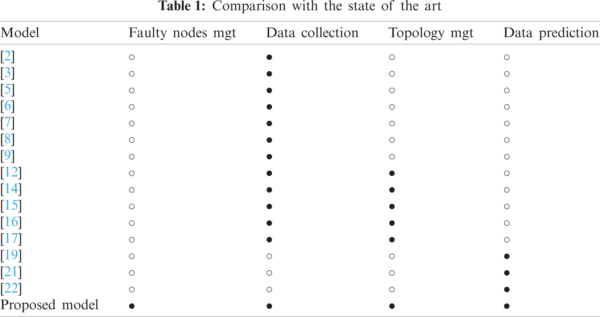
Although several works integrated UAVs and WSNs, it should be stressed that none of them make use of UAVs to enable higher-resilience WSNs during flood prediction or make evaluations based on real data. Concerning quick learning for UAV navigation tasks, some previous works typically emphasize accurate methods for components such as perception and relative pose estimation [10] or trajectory optimization and control [11]. UAVs can support various wireless communication protocols. For example, UAVs can communicate with WSNs in a self-organized way by ZigBee modules [12,13] and have the ability to serve as relays to forward data to the cloud [14–17]. These models include Artificial Neural Networks (ANNs), Genetic Programming (GP), Adaptive Neuro Fuzzy Inference Systems (ANFIS), and Support Vector Machines (SVM) to evaluate the longitudinal dispersion constant [18]. Among these techniques is the GMDH that is a self-organizing method with non-linear network models. It uses a combination of a quadratic polynomial in a multi-layer procedure [19]. Many recent algorithms such as GMDH networks have been able to perform accurate predictions, especially the river water stage prediction. The GMDH networks were a quick learning machine planned by Ivakhnenko in the 1960s [20,21]. The GMDH networks provide effective and efficient technical performance in various engineering fields [21], but their training suffers from certain disadvantages such as local minimum and slow convergence. Therefore, selecting an applicable training model is one of the paramount steps within the development of a data-driven model. This study adopted the PSO technique [20] to train GMDH networks for river prediction models. The developed model is a hybrid method for one-day-ahead prediction of river water where a non-linear regression approach is adopted due to the complex process of river flow prediction in natural rivers. It is evaluated in simulated networks in Malaysia, where some other neural network-based models, including DE, GA, and ANN, are also tested for comparison. The effective forecasting technique for river water stages would minimize losses from flooding exploitation due to the prediction of what people close to the river need [22–24]. Some limitations of the GMDH technique include slow convergence in training, imprecision in parameter assessment, overfitting, the partition of information, and low accuracy. Therefore, a hybrid version of GMDH was planned to considerably boost its performance. Robinson and colleagues [25] presented a Multi-Objective GMDH (MOGMDH) algorithm within a consistency criterion that used three different selectors within the choice procedure. This significantly improved the performance of the GMDH algorithmic program. Hiassat et al. [26] proposed the Genetic Programming-GMDH algorithmic program, which applies genetic programming to discover the simplest functions that can map inputs to outputs for every layer of the GMDH algorithmic program, and they presented a model that achieves better results than the standard GMDH algorithm in time series predictions using financial and weather information. Genetic Algorithms (GAs) have recently attracted attention in feedforward self-organizing networks. In this study, neuron connections are controlled to adjacent layers [27]. The lack of effective training algorithms for training multi-layer perceptron is an important issue in GMDH networks. In recent years, some data-driven improvements to training algorithms such as Back Propagation (BP) [28], Levenberg-Marquardt procedure [29], and scaled conjugate gradient procedure [30] have been used to perform training tasks. Usually, gradient-based methods have some drawbacks, such as slow speed convergence during training and getting trapped in local minimums. So far, several prediction approaches have been proposed. However, none of these approaches has taken into consideration the effect of data collection by UAVs for river flow prediction along with the PSO algorithm for training the GMDH model. We made a comparison to prove the novelty of the proposed model. The comparison with the state of the art is provided in Tab. 1. The table presents the proposed models that used UAVs for data collection from the sensor nodes using UAVs.

3  Problem Statement

In WSN-based flood monitoring approaches, nodes might be destroyed or get faulty during a flood that seriously affects the network connectivity. To overcome this issue, UAVs could be deployed to act as routers or data mules to fill the network communication gap caused by the inactive nodes. UAVs relay packets from the isolated nodes and enable continuous flood monitoring. In our UAV-assisted data collection mechanism, the WSN is modeled as an undirected graph as follows:

Let G=(V,E) be a simple connected and undirected graph, where V and E represent the vertex and the edge set, respectively. In the WSN, the sensor nodes $n$ and the wireless communication links m are modeled as vertices and edges, respectively. The set of vertices is represented as V={v1,v2,v3,…,vn} and set of edges E={e1,e2,e3,…,em} is expressed as the wireless communication links. The degree(vi) represents the degree of a vertex and shows the number of valid neighbors of a sensor node. The value of degree(vi) may change during the flood prediction process, due to the destroyed nodes. Also, the Valid neighbors are defined as nodes with valid wireless communication capability. Furthermore, we assume that each node possesses the information of its neighbors in a table that includes the connectivity status, neighbor node IDs and the radio signal strength indicator (RSSI) between the nodes. Matrix C shows the connectivity status between the nodes as follows:

According to the matrix, if e(vi,vj) exists, the vertices vi and vj can communicate. Otherwise, If there is no possibility for wireless communication between vi and vj, the UAV nodes is called to collect data from the node. To solve this problem, the sensor nodes are grouped into N sub-regions by the cloud using a number of beacons with known locations. Each sensor node records all the detected beacons, and selects the certain sub-region based on the highest RSS of the beacons’ signal. Then, the random walk process is applied for propagating data on a connected graph with n vertices and m edges at the sub-regions. Given K sensor nodes in a sub-region, the distance matrix is defined as D and the location of the first UAV hovering point is expressed as mlf and while the UAV moves to the mth location, the distance matrix is defined as mlm. With m recorded locations, the collected data of K sensor nodes can be predicted through the proposed flood prediction model.

4  Proposed Multi-level Architecture

Here, the details of the suggested architecture are explained. The proposed network model is an adaptable and scalable model with multiple applications. The model was designed with three layers. In the cloud-SDN layer, a centralized SDN controller was defined as the main control entity and the central processing unit for action predictions. The SDN controller linked the ground WSN and UAV. The second layer included UAVs operated on-demand, with progressive sensors and communication. The third layer covered ground WSNs with scalar sensors such as rainfall sensors and water level sensors. Fig. 1 shows the network model and the key components of the cloud-SDN, UAVs, and sensors. The main components of the suggested framework are presented in detail.

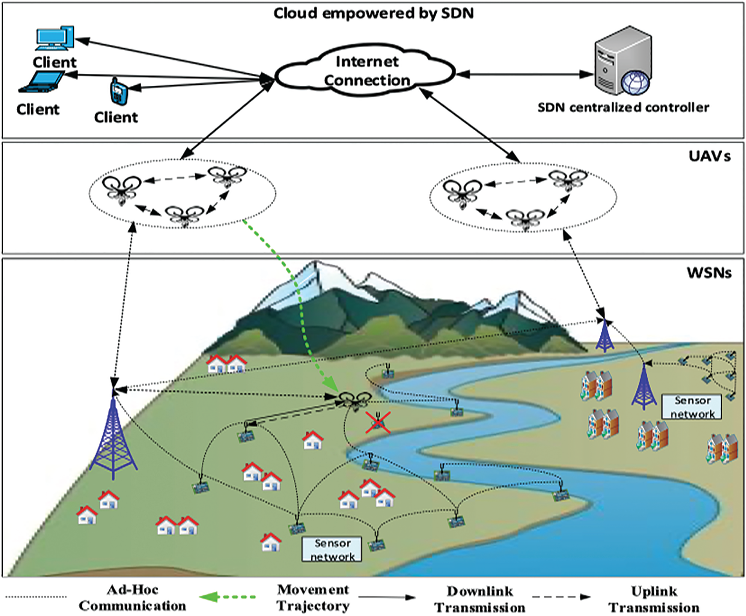
Figure 1: Proposed multi-level architecture

A communication network is an important component of the flood control system. With the integration of advanced technologies and applications for achieving smarter controlling of rivers, a vast amount of data from different locations will be generated for analysis, update, control, and real-time flood predicting methods. Thus, the management of these networks is the main challenge due to the scale. Moreover, the equipment may not be able to exchange information due to heterogeneous devices and applications. Hence, it is a vital issue to find the best communication infrastructure to control and manage all devices throughout the total system, considering the real-time constraint. In this model, cloud computing-based SDN is a good solution to the aforementioned problems, thanks to the following advantages. Cloud technology offers high computing capacity to flood prediction utilities. Moreover, flexible per flow routing is possible using SDN and the flow can be defined across multiple network layers. Also, a logically centralized controller can improve the service efficacy of flood prediction. Also, due to the programmability of SDN, the network is made more active and an appropriate radio access interface can be selected for data delivery. Last but not least, quick-response cloud service is essential for river monitoring on the basis of the real-time road conditions.

Generally, UAVs as aerial agents refer to active objects with behavior, state, and location, which are autonomous and mobile. They can move freely with state and code in execution without suspending services, provide better asynchronous interaction, reduce communication cost, and enhance flexibility. For greater geographical distances where ground nodes are infeasible, UAV-based systems can be integrated. UAVs collected data from the sensing targets and transmitted the collected data to the ground control station or terrestrial user equipment. Various reasons have been provided for the use of UAVs in the proposed network model. The main reason is that the employment of UAVs will lead to lower traffic over the wireless channel. Also, in comparison to traditional network forwarding, the reliability of the path will be significantly improved as the numbers of hops will be reduced where packets are diffused in the network over multiple hops. The direct communication, where the UAV collects data from each sensor node, is used for data acquisition.

The ground control station was configured for data analysis and to control management operations. Ground data was distributed between ground control stations and UAV communication nodes. Sensor nodes are flexible network elements that deliver (real-time) collected water level data to the central processing unit. However, considering the extremely large area and numerous working scenarios involved in flood control, it is impossible to manage floods without using UAVs as detection tools. These were generally controlled from the ground control station.

5  Prediction Model

In this section, the methodology for flood prediction using UAVs along with a PSO algorithm for training the GMDH model is described.

5.1 GMDH Approach

The GMDH method has various stages. The first stage involves partitioning data into training data and testing data. This division is based on consecutive heuristic selection points in the data set. Also, this partitioning is obtained by calculating the variance of data from the mean value. Points should have high variance and be employed in the testing data set for model checking, outside of the data in the training set. In the second step, input data for the input matrix was chosen in pairs and, between each pair, a quadratic polynomial was taken with the corresponding output. The least-square fitting [31–33] is used to set the polynomial coefficients. To verify polynomial's suitability, the outputs of the polynomials were evaluated using data points in the testing data. Mostly, Mean Squared Error (MSE) was used to select suitable polynomials for the next layer. Finally, this process was repeated until the smallest MSE was higher than the previous layer. A suitable data model was obtained by tracing back the polynomial path with the smallest MSE in each layer. The GMDH method relies on self-organizing methods for the assessment and estimation of recording machine models with uncertain variable relationships. GMDH networks use a regression based on the Ivakhnenko polynomial [34] as follows:

y=a0+∑i=1Maixi+∑i=1M∑j=1Maijxixj+∑i=1M∑j=1M∑k=1Maijkxixjxk (1)

where M is the number of input variables, (x1,x2,x3,…,xM) are the input variables; and (a0,ai,aij,aijk,…) are the coefficients. Generally, Eq. (1) is the quadratic form of the two variables shown in Eq. (2):

y=a0+a1xi+a2xj+a3xixj+a4xi2+a5xj2 (3)

The configuration of the GMDH model employed in this study is presented in Fig. 2.

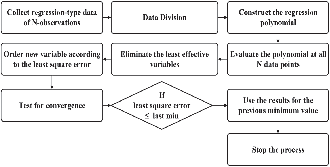
Figure 2: GMDH structure

5.2 The Proposed Hybrid GMDH–PSO Algorithm

The usual version of GMDH has some shortcomings that need to be addressed: (i) how to train two-layered high-precision networks; (ii) how to specify the best number of input variables; (iii) how to choose a polynomial order to form a vector solution in every node; and (iv) how to select input variables. This study focused on these issues using the proposed GMDH-PSO model.

5.2.1 Using PSO in the Training Process

It is apparent from previous sections that the GMDH method has some limitations in the training process. Hybridization of the PSO model with standard GMDH can solve this problem. In this application, a three-layered perceptron was chosen. PSO was used to train the GMDH network. Initially, the fitness function of every particle was determined. The error function at current particle positions was evaluated to determine the fitness value of every swarm particle. Also, fitness values were determined on the basis of the particle position vectors corresponding to the network weight matrix. In this hybrid technique, all training data was set to the GMDH network. Then, the weights of each data set were updated such that the size of the training set was equal to the number of updated weights. The vector of each particle was selected to show their error vector. This vector stored the minimum errors encountered by each particle due to their input patterns. This value shows the Mean Square Error (MSE) during training. The flowchart procedure for training a GMDH network using PSO is given in Fig. 3.

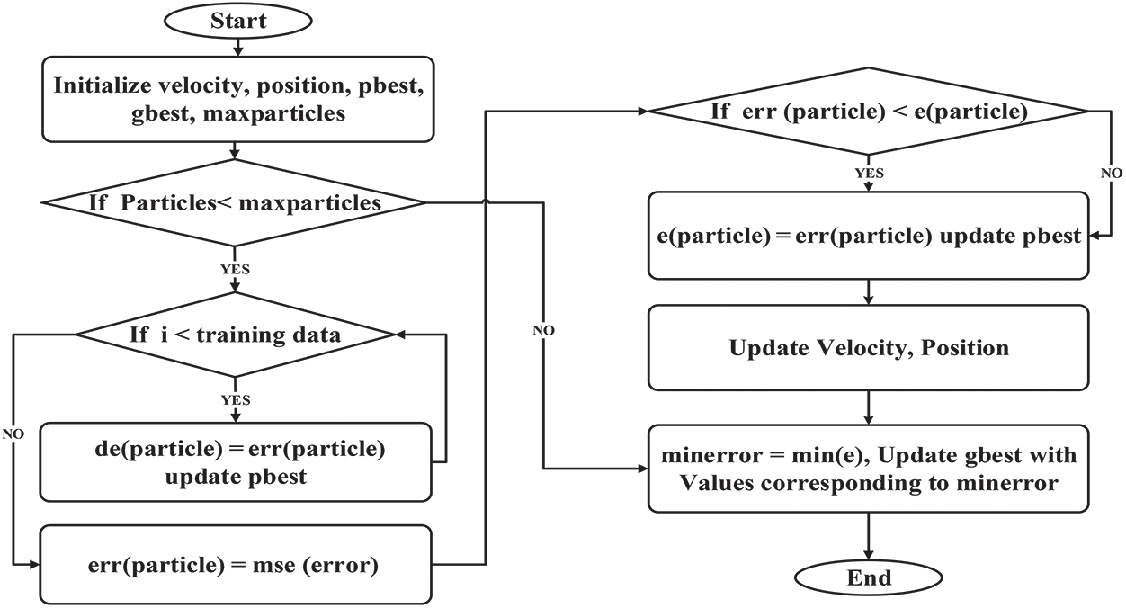
Figure 3: Architecture of the proposed SDN-EC framework

Weight training was used for the following reason: W1 shows the weight matrix between the input layer and the hidden layer; W2 denotes the weight connection matrix between the hidden layer and the output layer. The ith particle of a PSO in multi-layer perceptron training is denoted as follows:

Wi=(Wi1,Wi2) (4)

For every particle, the former best fitness value was defined to present the position of the particle as follows:

Pi=(Pi1,Pi2) (5)

The best particle index among all the particles in the population is shown by b and the best matrix is presented by:

Pb=(Pb1,Pb2) (6)

The particle velocity i is denoted by

Vi=(Vi1,Vi2) (7)

The formula for particle manipulation in each iteration is presented as follows:

Vi"[j](m,v)=Vi[j](m,v)(rα[Pi[j](m,v)−Wi[j](m,v)]+sβ[Pb[j](m,v)−Wb[j](m,v)])/t (8)

where m and n denote matrix rows and columns, respectively; r and s are positive constants; t is the time step between observations and is commonly taken as unity; α and β are random numbers from 0 to 1; V and W refer to the new values.

Wi"[j]=Wi[j]+Vi[j]t (9)

where j=1,2; m=1,…,Mj; n=1,…,Nj; Mj and Nj are the rows and column sizes of the matrices W, P, and V. Eq. (5). was utilized to compute new particle velocities based on its previous velocity and the distance of its current position from its best experience and the best experience of its group. Then, a new position according to the new velocity is determined using Eq. (5). Also, Eq. (6) was used to determine the fitness of the ith particle in terms of an output mean squared error of the neural network as follows:

f(Wi)=1S∑k=1S[∑l=1O{tkl−pkl(Wi)}2] (10)

In the above equation, the fitness value is f; the target output is tkl; the number of output neurons is O; the predicted output according to Wi is pkl; the number of training set is S.

5.2.2 Region and Data Description

Hydrographs offered daily water level records from Selangor River via http://infobanjir.water. https://gov.my. The Selangor River is the main river in Selangor, Malaysia. It runs from Kuala Kubu Bharu in the east and flows into the Straits of Malacca at Kuala Selangor in the west. The data presented through this website were suitable indicators of potential flooding or landslides. This study utilized the data from this website with discretion. This study extracted online hydrograph data for three stations—Selangor, Selayang, and Bernam—on the Selangor River. According to the existing hydrographs on 27 December 2018, the average water level measured by Station1 was about 48.72. These values were about 37, 44, and 21 for Station1, Station2, and Station3, respectively.

5.2.3 Data Normalization

The water levels data set at the Selangor river were predicted over one and two days based on measured daily levels. Data normalization was done to avoid false patterns that can be created by inconsistencies. The dataset had some variations because the collection devices were located in different time zones and geographical locations. Data were normalized by dividing the total daily water levels by the number of hours within that day. The normalized data series were computed as:

Dt′=DtHt (11)

where Dt is total daily water level, Dt′ is the normalized data, and Ht is the number of hours in the ith day.

5.2.4 Construction of Polynomials by PSO

Particles were used as search agents in the PSO. The grouping of input variables from the previous layer was determined on the basis of the position of each particle. This data was then moved to the next layer. Every particle contained three main parameters: P1, P2, and P3. P1 was defined as a polynomial order. In this context, the polynomial order was created from the previous layers and generated randomly. For simplicity, this study took 2 in each layer. However, this value can be either 2 or 3. The number of input variables was generated randomly and was obtained from the previous layer. We defined D and r=2 as the width of the input dataset and the default lower bound, respectively. The number of input variables was P2∈[1,r], where r=min(D,5). The position of every particle representing tall candidates in the current layer of the network was P3={a∈Z+|1≤a≤D}, which is a sequence of integers. These three parameters were used to arrange nodes to move to the next layer. P1, P2, and P3 were used to determine the polynomial order, the number of node groupings, and the whole sequence, respectively. Fig. 4 shows the procedure for the three defined parameters used to form the polynomial. In our hybrid model, three parameters were used to create the polynomial and all particles consisted of separate parameter sets. Generated polynomials were employed as an objective function for PSO.

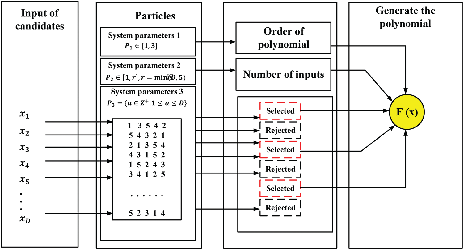
Figure 4: Construction of polynomials by PSO

5.2.5 Framework of the GMDH-PSO

The GMDH-PSO framework is comprised of six main steps: First, the input variables of the system were determined. The primary population of PSO structures and corresponding learning parameters c1 and c2 were created. The input variables of the model were defined as xi; (i=1,2,3,…,n) and were related to output variable y. Then, the normalization of input data was completed. In both experiments, the original data needed to be normalized to generate equivalent water level data. In the second phase, training data for PSO and testing data was formed. The input-output data set (xi,yi)=(x1i,x2i,…,xni,yi); i=1,2,3,…,n was divided into a training and testing dataset. The size of the training and testing dataset were represented by ntr and nte, respectively, where $n=ntr+nte. The training dataset was employed to construct the GMDH-PSO model. The testing dataset was utilized to evaluate model quality. In the third phase, the primary information that would be used to construct the GMDH-PSO structure was determined. Note that the previously mentioned process determined the model’s structural optimization by PSO variation operators. In this context, we defined the maximum number of generations as the termination method to balance model accuracy and complexity. The maximum number of input variables was used for every node in each layer. Moreover, the value of the weighting factor was determined for the aggregate objective function. In the fourth phase, the Polynomial Neuron (PN) structure was determined using the PSO algorithm. The least-square technique was used for parameter optimization through multiple-regression analysis. This technique was used to provide the formula to compute coefficients. The objective function, which was the main instrument used to control evolutionary searches in the solution space, was defined based on the following generated polynomial:

f(x1,x2)=a1+a2x1+a3x2+a4x1x2+a5x12+a6x22 (12)

where a1,a2,…,a6 are the constants assessed using the training dataset. The formula used to compute coefficients was obtained using the least-square method in the following formula: a=(xtx)−1xty. In the fifth phase, if the current structure was the best, the model proceeded to phase 6, otherwise it returned to phase 3. This procedure was repeated for all nodes at all layers (from the input layer to the output layer). In the sixth phase, if an acceptable solution was obtained, then the algorithm was stopped, otherwise the model returned to step 2. The GMDH-PSO algorithm was carried out by consecutively repeating steps 2–6. When the termination condition was met, one solution vector with the optimum performance was selected in the last population generation as a solution vector and all remaining solution vectors were rejected. The pseudocode of GMDH-PSO is represented in Algorithm 1. Besides, Fig. 5 shows the GMDH-PSO model.

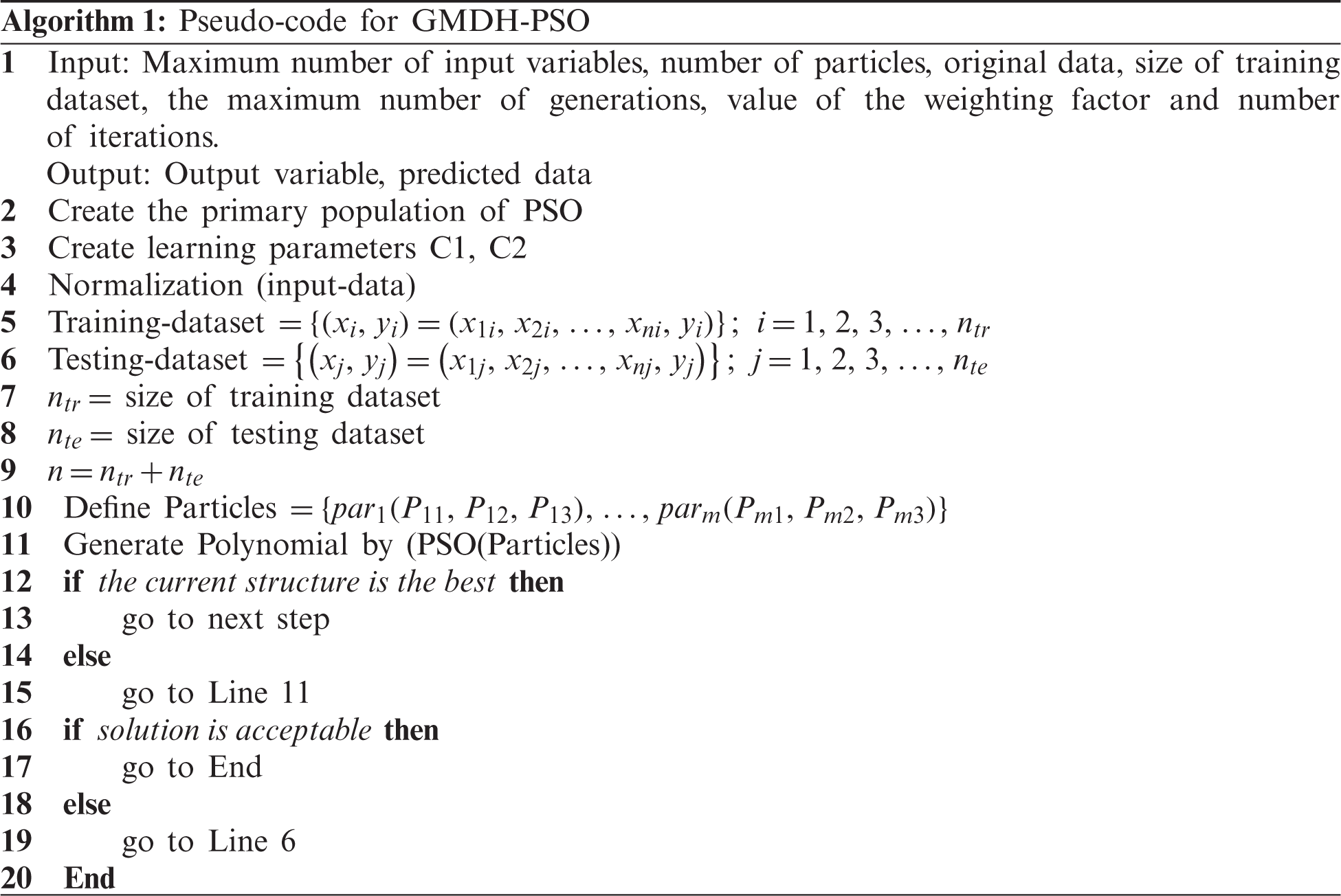
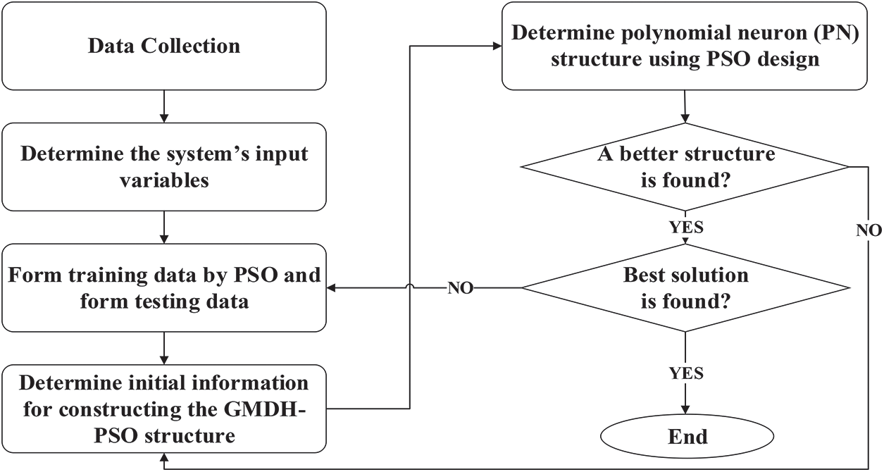
Figure 5: Construction of polynomials by PSO

6  Results

The GMDH-PSO network was compared with earlier models such as DE [35], GA [36], and ANN [37] and the results are presented in this section. In these comparisons, the main indicators for prediction errors were calculated for model evaluation [38]. In this regard, we utilized the raw data related to river level values over 24 hours from three different stations. This study used the correlation coefficient R, RMSE, and BIAS data for accuracy evaluation in the training and testing stages as follows:

R=∑i=1M(Yi(Original−Y¯(Original))(Yi(Model)−Y¯(Model))∑i=1M(Yi(Original)−Y¯(Original})2.∑i=1M(Yi(Model)−Y¯i(Model))2 (13)

RMSE=[∑i=1M|(Yi(Model)−Yi(Original))2|M]12 (14)

BIAS=∑i=1M(Yi(Model)−Yi(Original))M (15)

where M refers to total events, Y¯(Model) refers to the mean of the predicted values, Yi(Original) was target data that showed the observed values, and Y¯(Original) was the mean of the observed values. The results for the statistical parameters show that the GMDH-PSO model was in good agreement with previously published methods. Also, the model obtained a precise prediction for the training phase. The values of R and RMSE were equal to 0.96 and 0.167, respectively. BIAS showed good precision in GMDH-PSO training equal to 4.82. The R and RMSE values were equal to 0.96 and 0.167, respectively. BIAS (equal to 4.82) showed good precision in GMDH-PSO training. The obtained values (R=0.89, RMSE=0.24, and BIAS=4.11) proved the high performance and efficiency of the proposed model during testing. Tab. 2 displays the results of the proposed model for the training and testing phases. In comparison, the R values from the testing phase were not significantly different from those for the training stage. On the contrary, BIAS and RMSE were noticeably improved parameters. Tab. 2 indicates the accuracy of the obtained results.

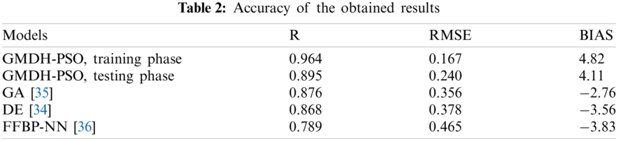
A comparison of the GA and DE models was performed for GMDH-PSO. The results showed that the appearance of the GA technique was more accurate than that of the DE model. The values for RMSE and BIAS were equal to 0.356 and –2.76, respectively, for the GA model, and 0.378 and -3.56, respectively, for the DE model. The BIAS for the DE model is smaller than the GA model, but the RMSE for the DE model is very similar to the GA model. Our proposed model showed better results in terms of BIAS compared to the DE and GA models. The GMDH-PSO model exhibited RMSE values approximately 20% lower than the DE and GA models. The ANN-based model was used for evaluation analysis. This study developed a Feedforward Backpropagation (FFBP) model for water level prediction. In this model, it was assumed that the proposed network had three hidden layers and that each layer had four neurons. This study found that the FFBP-NN technique had more accurate predictions with RMSE=0.465 and BIAS=−3.83 compared to the DE model. Although, the FFBPNN model, compared to the GA model, obtained more errors. In total, the GMDH-PSO model showed shows slightly better performance than the GA model in terms of accuracy. The predicted and measured data of Station 1, Station 2, and Station 3 for the proposed models are shown, respectively, in Figs. 8–10 (Appendix A).

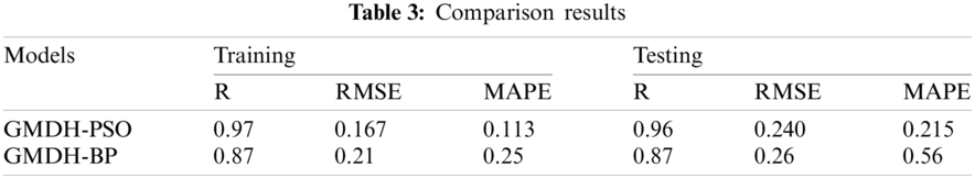
Here, we evaluate the performance of GMDH-PSO and GMDH-BP during the training and testing phases. Model evaluation statistics were MAPE (Mean Absolute Percentage of Error), R, RMSE:

MAPE=1M[∑i=1M|Yi(Model)−Yi(Original)|∑i=1MYi(Original)×100] (16)

whereas predicted value network output is Yi(Model), average predicted values are Y¯(Model), observed values are Yi(Original), average observed values are Y¯(Original), and M is the total number of events. The training phase shows that the use of the PSO model as a trainer of the GMDH network provided better performance than the use of a back-propagation algorithm. The R values for the GMDH-PSO and GMDHBP models were 0.97 and 0.86, respectively. The RMSE for GMDH-PSO and GMDH-BP were 0.167 and 0.24, respectively. The MAPE values were 0.113 for the GMDH-PSO model and 0.215 for the GMDH-BP model. The GMDH-GP model had a complicated structure because of the creation of tree structures in each neuron, making this procedure very time-consuming. The testing phase indicated that GMDH-PSO had better performance than GMDH-BP in terms of accuracy. This study used the remaining data sets for testing performances. The R value for GMDH-PSO was 0.96 and the GMDH-GP model was 0.87. The RMSE and MAPE for the GMDH-PSO model were smaller than the GMDH-BP model. Tab. 3 shows the comparison results.

7  Simulation Validation

In this section, we discussed some experiments conducted to demonstrate the accuracy of our proposed model, and the obtained results were analyzed. These experiments were conducted to implement self-developed UAV-WSN modules, which were simulated with the OMNET++ tool. In our system, each sensor directly communicates with the UAVs to save energy and decrease the end to end communication delays. This study assumed that the active sensor nodes would communicate with UAVs if they were within the range of the beacon signal. Furthermore, the slept sensor node did not communicate if the beacon signal was weaker than the threshold or the beacon signal was not available. During data collection, this study assumed that each active sensor could periodically transmit sensing data to the UAVs. Tab. 4 shows all the parameters used in our simulations and two sets of valuations.

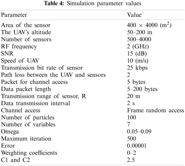
To perform competition experiments, this study carried out different experiments under different experimental conditions. In the first experiment, every sensor node always transmitted a packet between the client and the server. In the second experiment, UAV carried out routing and packet switching between the source node and destination node. In this experiment, if a sensor node failed, former sensor nodes could not send their data to the sink node. By employing UAVs, the data collection was possible throughout the WSN, which sent data to the central processing unit for river prediction. In this context, performance evaluations were evaluated with two response variables: Round-Trip Time (RTT) delay and packet loss rate. RTT refers to how long it took for a packet to be sent back and forth from the source to the destination. Packet loss rate refers to the ratio of packets lost in the test to the data groups sent during transmissions. Besides, each experimental result is the average of the 30 runs for each simulation scenario. The 95% confidence interval (CI) has been calculated for the collected performance metrics unless they (CI) are profoundly small. To this end, the parameter values used in this study are shown in Tab. 4. These values were carefully selected to reflect realistic scenarios.

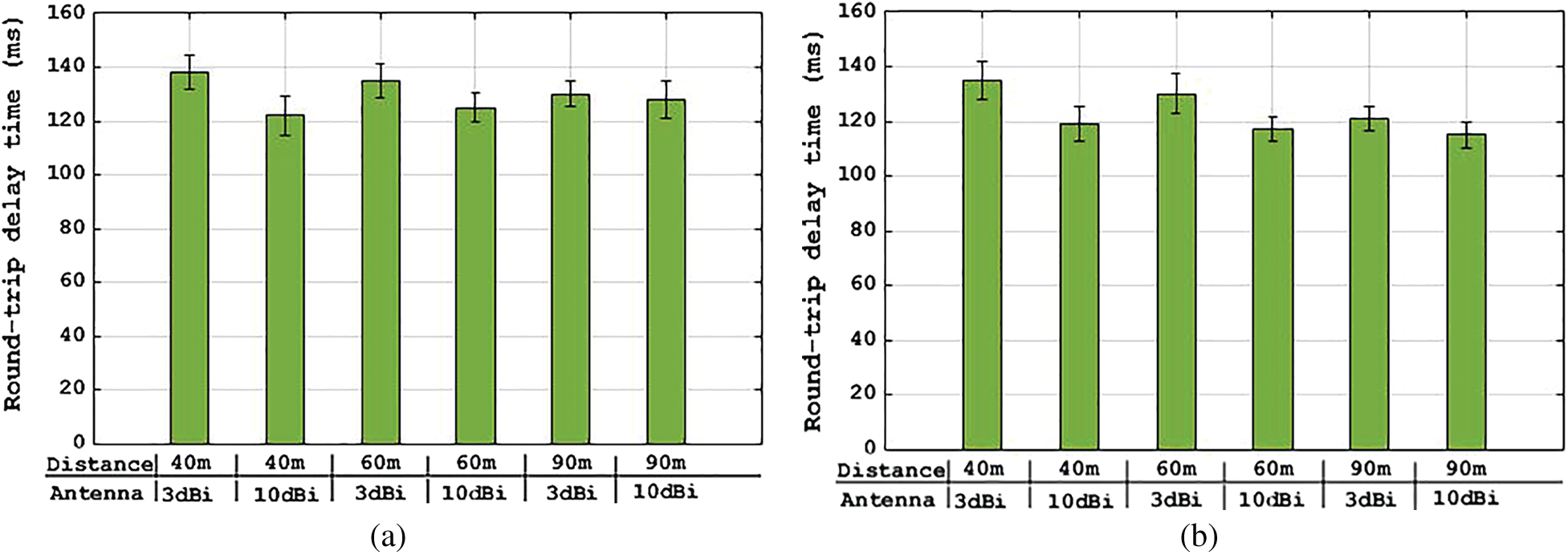
Figure 6: Results (a) and (b) of round-trip time (RTT) delay (a) Without UAVs (b) With UAVs

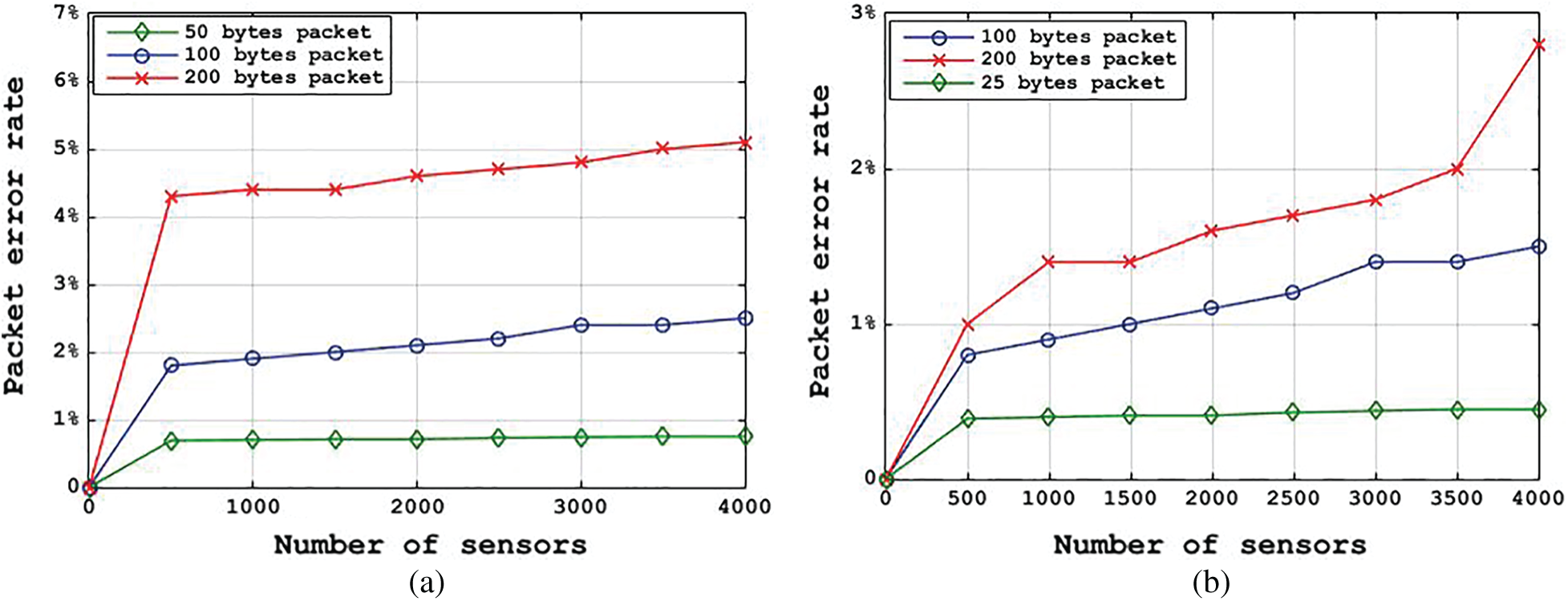
Figure 7: Results (a) and (b) of the packet loss rate (a) Without UAVs (b) With UAVs

Figs. 6 and 7 show the results of these two experiments: Experiment without UAVs and experiment with UAVs. The two sets of experiments were simulated thirty-five times, and the Shapiro–Wilk normality test was used to test the normality of experiment sets.

The experiment results showed that UAVs can improve the data collection and provide a reasonably well depiction of remotely sensed environments. Compared with the existing efforts {[35–38]}, the main advantage of this study is to design a UAV-WSN model for river flow prediction.

8  Conclusions and Future Directions

This study used UAV remote sensing for scenarios where a sensor node is unable to send data packets in multi-hop communications to provide robust WSNs. The usage of UAVs can improve the accuracy of water level predictions to prevent floods. Experiments tested data collection performance with and without UAVs for river monitoring. This study’s UAV-WSN model proposed the hybridization of the PSO and GMDH models for water level predictions. To validate the precision of the developed GMDH-PSO model, its performance was compared to the DE, GA, and ANN models. The GMDH-PSO method outperformed the other models. The statistical indicators used for the performance evaluation of the proposed model indicated lower RMSE and higher R and BIAS compared to the GA and DE models for all nodes. Also, this study compared GMDH-PSO and GMDH-BP during the training and testing stages. The outcomes showed that MAPE was lower in the GMDH-PSO model. Results underlined the ability of GMDH-PSO to predict non-linear time series data. For future works, this study recommends the use of other techniques to predict river water levels such as reinforcement learning. In future research, to improve the computation services while reducing the latency, we plan to apply edge computation (EC). Additionally, we will consider forecast of different environmental phenomena, such as urban underground drainage or rainfall-flow.

Funding Statement: This work was supported by Ministry of Higher Education, Fundamental Research Grant Scheme, Vote Number 21H14, and Faculty of Information Science and Technology, Universiti Kebangsaan Malaysia (Grant ID: GGPM-2020-029 and Grant ID: PP-FTSM-2020).

Conflicts of Interest: The authors declare that they have no conflicts of interest to report regarding the present study.

References

 1.  R. Khatibi, S. Bellie, M. A. Ghorbani, O. Kisi, K. Koçak et al., “Investigating chaos in river stage and discharge time series,” Journal of Hydrology, vol. 414, no. 1, pp. 108–117, 2012. [Google Scholar]

 2.  D. Freitas, E. Pignaton, T. Heimfarth, I. F. Netto, C. E. Lino et al., “UAV relay network to support WSN connectivity,” in Int. Congress on Ultra-Modern Telecommunications and Control Systems. Moscow, Russia, pp. 309–314, 2010. [Google Scholar]

 3.  G. Tuna, T. V. Mumcu, K. Gulez, V. C. Gungor and H. Erturk, “Unmanned aerial vehicle-aided wireless sensor network deployment system for post-disaster monitoring,” in Int. Conf. on Intelligent Computing, Huangshan, China, pp. 298–305, 2012. [Google Scholar]

 4.  M. H. Anisi, A. Hanan Abdullah and S. Abd Razak, “Energy-efficient and reliable data delivery in wireless sensor networks,” Wireless Networks, vol. 19, no. 4, pp. 495–505, 2013. [Google Scholar]

 5.  J. Valente, D. Sanz, A. Barrientos, J. Del Cerro, Á. Ribeiro et al., “An air-ground wireless sensor network for crop monitoring,” Sensors, vol. 11, no. 6, pp. 6088–6108, 2011. [Google Scholar]

 6.  Sh. Goudarzi, N. Kama, M. H. Anisi, Sh. Zeadally and Sh. Mumtaz, “Data collection using unmanned aerial vehicles for internet of things platforms,” Computers & Electrical Engineering, vol. 75, no. 1, pp. 1–15, 2019. [Google Scholar]

 7.  J. Ueyama, H. Freitas, B. S. Faiçal, P. R. Geraldo Filho, P. Fini et al., “Exploiting the use of unmanned aerial vehicles to provide resilience in wireless sensor networks,” IEEE Communications Magazine, vol. 52, no. 12, pp. 81–87, 2014. [Google Scholar]

 8.  I. Jawhar, N. Mohamed and J. Al-Jaroodi, “UAV-based data communication in wireless sensor networks: Models and strategies,” in Int. Conf. on Unmanned Aircraft Systems (ICUASDenver Marriott Tech Center, Denver, Colorado, USA, pp. 687–694, 2015. [Google Scholar]

 9.  P. Sun, A. Boukerche and Q. Wu, “Theoretical analysis of the target detection rules for the UAV-based wireless sensor networks,” in IEEE Int. Conf. on Communications (ICCPorte Maillot, Paris, France, pp. 1–6, 2017. [Google Scholar]

10. E. H. Beck, N. Vergopolan, M. Pan, V. Levizzani, I. A. Van Dijk et al., “Global-scale evaluation of 22 precipitation datasets using gauge observations and hydrological modelling,” Hydrology and Earth System Sciences, vol. 21, no. 12, pp. 6201–6217, 2017. [Google Scholar]

11. A. Rucco, P. B. Sujit, A. P. Aguiar, J. B. De Sousa and F. L. Pereira, “Optimal rendezvous trajectory for unmanned aerial-ground vehicles,” IEEE Transactions on Aerospace and Electronic Systems, vol. 54, no. 2, pp. 834–847, 2017. [Google Scholar]

12. A. Shaw and K. Mohseni, “A fluid dynamic based coordination of a wireless sensor network of unmanned aerial vehicles: 3-D simulation and wireless communication characterization,” IEEE Sensors Journal, vol. 11, no. 3, pp. 722–736, 2010. [Google Scholar]

13. E. Milan, E. Natalizio, K. R. Chowdhury and I. F. Akyildiz, “Help from the sky: Leveraging UAVs for disaster management,” IEEE Pervasive Computing, vol. 16, no. 1, pp. 24–32, 2017. [Google Scholar]

14. M. Mozaffari, W. Saad, M. Bennis and M. Debbah, “Mobile unmanned aerial vehicles (UAVs) for energy-efficient Internet of Things communications,” IEEE Transactions on Wireless Communications, vol. 16, no. 11, pp. 7574–7589, 2017. [Google Scholar]

15. N. Goddemeier, K. Daniel and C. Wietfeld, “Role-based connectivity management with realistic air-to-ground channels for cooperative UAVs,” IEEE Journal on Selected Areas in Communications, vol. 30, no. 5, pp. 951–963, 2012. [Google Scholar]

16. L. R. Pinto, A. Moreira, L. Almeida and A. Rowe, “Characterizing multihop aerial networks of cots multirotors,” IEEE Transactions on Industrial Informatics, vol. 13, no. 2, pp. 898–906, 2017. [Google Scholar]

17. T. Yu, X. Wang, J. Jin and K. McIsaac, “Cloud-orchestrated physical topology discovery of large-scale IoT systems using UAVs,” IEEE Transactions on Industrial Informatics, vol. 14, no. 5, pp. 2261–2270, 2018. [Google Scholar]

18. H. Md. Azamathulla and F. Ch. Wu, “Support vector machine approach for longitudinal dispersion coefficients in natural streams,” Applied Soft Computing, vol. 11, no. 2, pp. 2902–2905, 2011. [Google Scholar]

19. M. Najafzadeh and A. MA Sattar, “Neuro-fuzzy GMDH approach to predict longitudinal dispersion in water networks,” Water Resources Management, vol. 29, no. 7, pp. 2205–2219, 2015. [Google Scholar]

20. J. Kennedy and R. C. Eberhart, “A discrete binary version of the particle swarm algorithm,” in IEEE Int. Conf. on Systems, Man, and Cybernetics, Computational Cybernetics and Simulation, Orlando, FL, USA, pp. 4104–4108, 1997. [Google Scholar]

21. M. Najafzadeh, Gh.-A. Barani and M. R. Hessami Kermani, “Aboutment scour in live-bed and clear-water using GMDH Network,” Water Science and Technology, vol. 67, no. 5, pp. 1121–1128, 2013. [Google Scholar]

22. F. Kalantary, H. Ardalan and N. Nariman-Zadeh, “An investigation on the Su-NSPT correlation using GMDH type neural networks and genetic algorithms,” Engineering Geology, vol. 104, no. 1–2, pp. 144–155, 2009. [Google Scholar]

23. J. Li and S. Tan, “Nonstationary flood frequency analysis for annual flood peak series, adopting climate indices and check dam index as covariates,” Water Resources Management, vol. 29, no. 15, pp. 5533–5550, 2015. [Google Scholar]

24. H. Qi, P. Qi and M. S. Altinakar, “GIS-based spatial Monte Carlo analysis for integrated flood management with two-dimensional flood simulation,” Water Resources Management, vol. 27, no. 10, pp. 3631–3645, 2013. [Google Scholar]

25. C. Robinson, “Multi-objective optimisation of polynomial models for time series prediction using genetic algorithms and neural networks,” Ph.D. dissertation. University of Sheffield, 1998. [Google Scholar]

26. J. Gascón-Moreno, S. Salcedo-Sanz, B. Saavedra-Moreno, L. Carro-Calvo and A. Portilla-Figueras, “An evolutionary-based hyper-heuristic approach for optimal construction of group method of data handling networks,” Information Sciences, vol. 247, no. 1, pp. 94–108, 2013. [Google Scholar]

27. H. Razzaghi, R. Madandoust and H. Aghabarati, “Point-load test and UPV for compressive strength prediction of recycled coarse aggregate concrete via generalized GMDH-class neural network,” Construction and Building Materials, vol. 276, no. 1, pp. 122–143, 2021. [Google Scholar]

28. Y. Hirose, K. Yamashita and Sh. Hijiya, “Back-propagation algorithm which varies the number of hidden units,” Neural networks, vol. 4, no. 1, pp. 61–66, 1991. [Google Scholar]

29. G. Lera and M. Pinzolas, “Neighborhood based Levenberg-Marquardt algorithm for neural network training,” IEEE Transactions on Neural Networks, vol. 13, no. 5, pp. 1200–1203, 2002. [Google Scholar]

30. M. F. Møller, “A scaled conjugate gradient algorithm for fast supervised learning,” Neural Networks, vol. 6, no. 4, pp. 525–533, 1993. [Google Scholar]

31. M. Clerc and J. Kennedy, “The particle swarm-explosion, stability, and convergence in a multidimensional complex space,” IEEE Transactions on Evolutionary Computation, vol. 6, no. 1, pp. 58–73, 2002. [Google Scholar]

32. M. Skoczylas, “Vision analysis system for autonomous landing of micro drone,” Acta Mechanica et Automatica, vol. 8, no. 4, pp. 199–203, 2014. [Google Scholar]

33. N. Ya’acob, N. Yusop, K. K. Mohd Shariff, A. L. Yusof, M. Tarmizi Ali et al., “Observation of tweek characteristics in the mid-latitude D-region ionosphere,” in IEEE Sym. on Wireless Technology and Applications, Bandung, Indonesia, pp. 27–31, 2012. [Google Scholar]

34. A. G. Ivakhnenko, “Polynomial theory of complex systems,” IEEE Transactions on Systems, Man, and Cybernetics: Systems, vol. 1, no. 4, pp. 364–378, 1971. [Google Scholar]

35. X. Li, H. Liu and M. Yin, “Differential evolution for prediction of longitudinal dispersion coefficients in natural streams,” Water Resources Management, vol. 27, no. 15, pp. 5245–5260, 2013. [Google Scholar]

36. R. R. Sahay and S. Dutta, “Prediction of longitudinal dispersion coefficients in natural rivers using genetic algorithm,” Hydrology Research, vol. 40, no. 6, pp. 544–552, 2009. [Google Scholar]

37. A. O. Anele, Y. Hamam, A. M. Abu-Mahfouz and E. Todini, “Overview, comparative assessment and recommendations of forecasting models for short-term water demand prediction,” Water, vol. 9, no. 11, pp. 887, 2017. [Google Scholar]

38. S. A. Soleymani, Sh. Goudarzi, M. H. Anisi, W. Haslina Hassan, M. Yamani Idna Idris et al., “A novel method to water level prediction using RBF and FFA,” Water Resources Management, vol. 30, no. 9, pp. 3265–3283, 2016. [Google Scholar]

Appendix A.

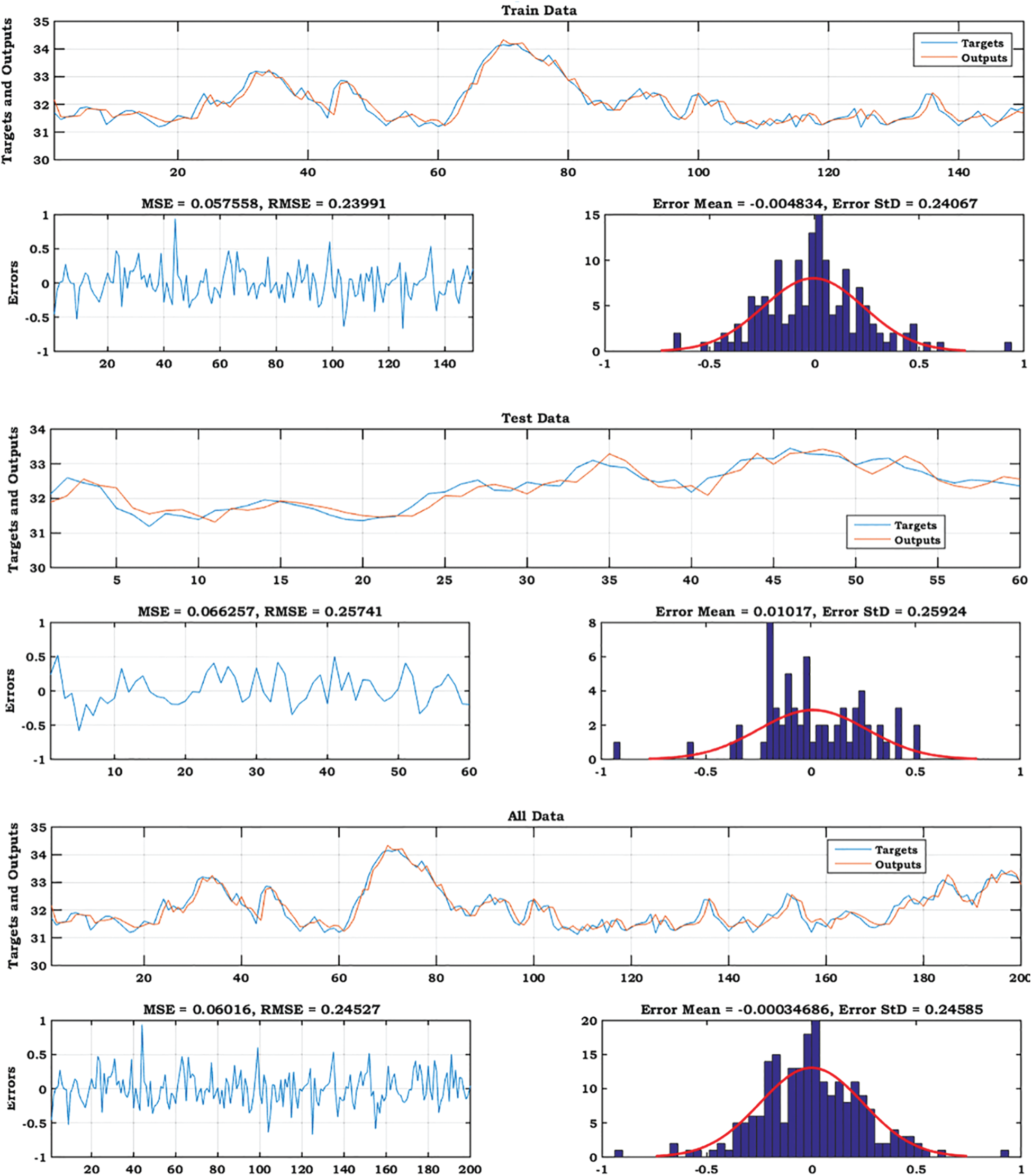
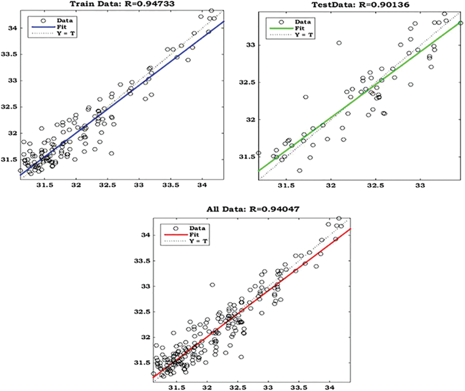
Figure 8: The plots of GMDH-PSO model predicted vs. actual values for training, testing and all data sets for Station 1

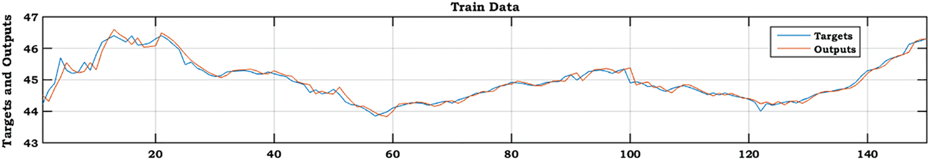
Figure 9: The plots of GMDH-PSO model predicted vs. actual values for training, testing and all data sets for Station 2

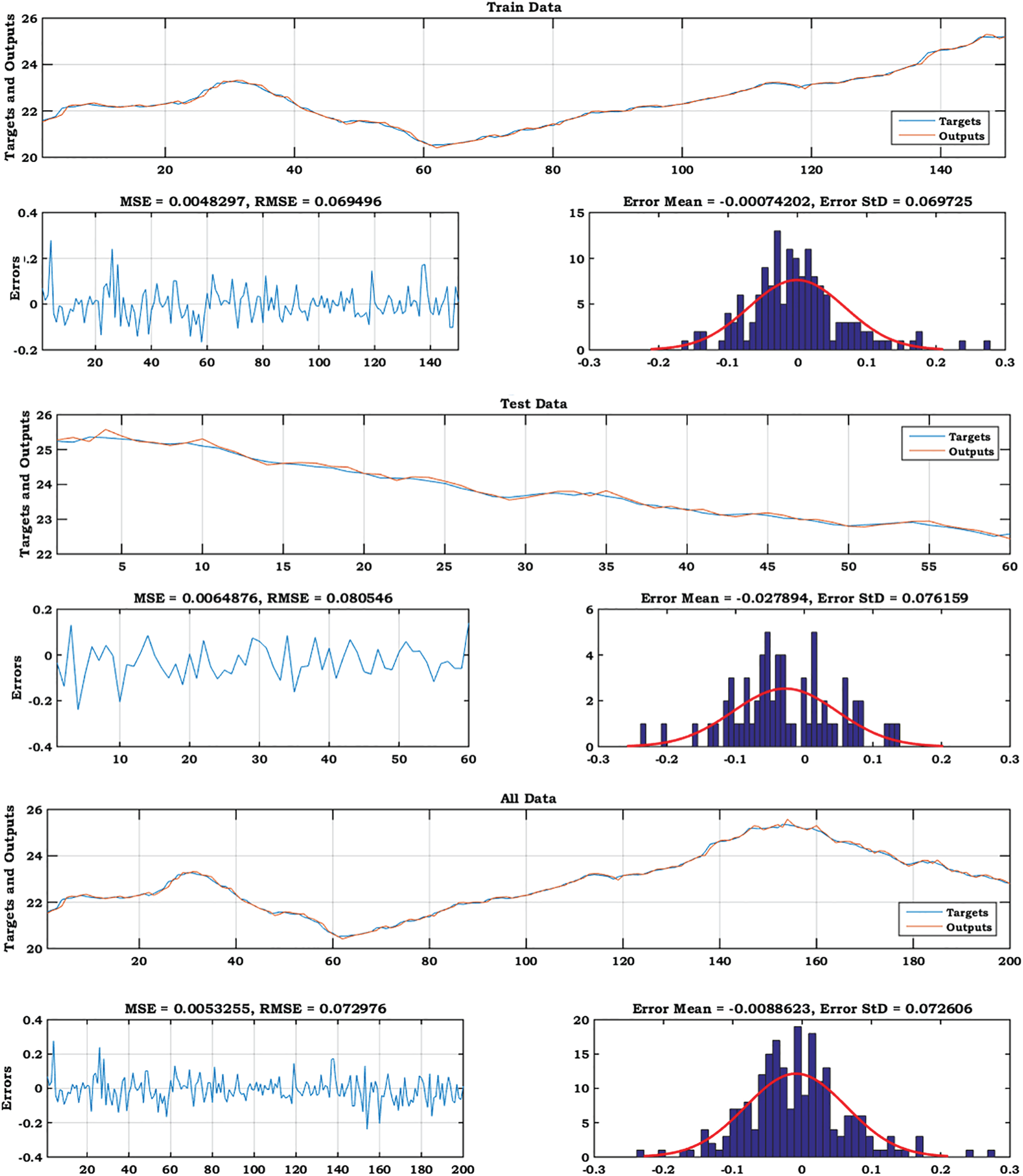
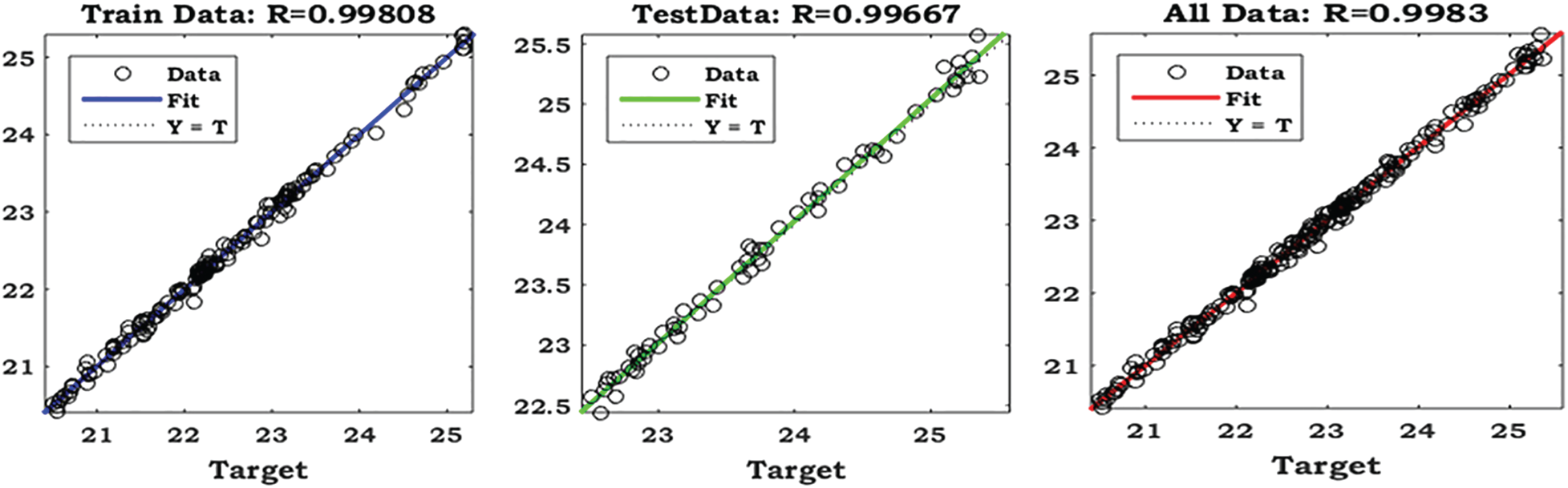
Figure 10: The plots of GMDH-PSO model predicted vs. actual values for training, testing and all data sets for Station 3

This work is licensed under a Creative Commons Attribution 4.0 International License, which permits unrestricted use, distribution, and reproduction in any medium, provided the original work is properly cited.