Computers, Materials & Continua DOI:10.32604/cmc.2022.019776
Article

Using Link-Based Consensus Clustering for Mixed-Type Data Analysis

Tossapon Boongoen and Natthakan Iam-On*

Center of Excellence in Artificial Intelligence and Emerging Technologies, School of Information Technology, Mae Fah Luang University, Chiang Rai, 57100, Thailand
*Corresponding Author: Natthakan Iam-On. Email: natthakan@mfu.ac.th
Received: 25 April 2021; Accepted: 06 June 2021

Abstract: A mix between numerical and nominal data types commonly presents many modern-age data collections. Examples of these include banking data, sales history and healthcare records, where both continuous attributes like age and nominal ones like blood type are exploited to characterize account details, business transactions or individuals. However, only a few standard clustering techniques and consensus clustering methods are provided to examine such a data thus far. Given this insight, the paper introduces novel extensions of link-based cluster ensemble, LCEWCT and LCEWTQ that are accurate for analyzing mixed-type data. They promote diversity within an ensemble through different initializations of the k-prototypes algorithm as base clusterings and then refine the summarized data using a link-based approach. Based on the evaluation metric of NMI (Normalized Mutual Information) that is averaged across different combinations of benchmark datasets and experimental settings, these new models reach the improved level of 0.34, while the best model found in the literature obtains only around the mark of 0.24. Besides, parameter analysis included herein helps to enhance their performance even further, given relations of clustering quality and algorithmic variables specific to the underlying link-based models. Moreover, another significant factor of ensemble size is examined in such a way to justify a tradeoff between complexity and accuracy.

Keywords: Cluster analysis; mixed-type data; consensus clustering; link analysis

1  Introduction

Cluster analysis has been widely used to explore the structure of a given dataset. This analytical tool is usually employed in the initial stage of data interpretation, especially for a new problem where prior knowledge is limited. The goal of acquiring knowledge from data sources has been a major driving force, which makes cluster analysis one of the highly active research subjects. Over several decades, different clustering techniques are devised and applied to a variety of problem domains, such as biological study [1], customer relationship management [2], information retrieval [3], image processing and machine vision [4], medicine and health care [5], pattern recognition [6], psychology [7] and recommender system [8]. In addition to these, the recent development of clustering approaches for cancer gene expression data has attracted a lot of interests amongst computer scientists, biological and clinical researchers [9,10].

Principally, the objective of cluster analysis is to divide data objects (or instances) into groups (or clusters) such that objects in the same cluster are more similar to each other than to those belonging to different clusters [11]. Objects under examination are normally described in terms of object-specific (e.g., attribute values) or relative measurements (e.g., pairwise dissimilarity). Unlike supervised learning, clustering is ‘unsupervised’ and does not require class information, which is typically achieved through a manual tagging of category labels on data objects, by domain expert(s). While many supervised models inherently fail to handle the absence of data labels, data clustering has proven effective for this burden. Given its potential, a large number of research studies focus on several aspects of cluster analysis: for instance, dissimilarity (or distance) metric [12], optimal cluster numbers [13], relevance of data attributes per cluster [14], evaluation of clustering results [15], cluster ensemble or consensus clustering [9], clustering algorithms and extensions for particular type of data [16]. Specific to the lattermost to which this research belongs, only a few studies have concentrated on clustering of mixed-type (numerical and nominal) data, as compared to the cases of numeric and nominal only counterparts.

At present, the data mining community has encountered a challenge from large collections of mixed-type data like those collected from banking and health sectors: web/service access records and biological-clinical data. As for the domain of health care, microarray expressions and clinical details are available for cancer diagnosis [17]. In response, a few clustering techniques have been introduced in the literature for this problem. Some simply transform the underlying mixed-type data to either numeric or nominal only format, with which conventional clustering algorithms can be reused. In particular to this view, k-means [18] is a typical alter- native for the numerical domain, while dSqueezer [19] that is an extension of Squeezer [20] has been investigated for the other. Other attempts focus on defining a distance metric that is effective for the evaluation of dissimilarity amongst data objects in a mixed- type dimensional space. These include different extensions of k-means, k-prototypes [21] and k-centers [22], respectively.

Similar to most clustering methods, the aforementioned models are parameterized, thus achieving optimal performance may not be possible across diverse data collections. At large, there are two major challenges inherent to mixed-type clustering algorithms. First, different techniques discover different structures (e.g., cluster size and shape) from the same set of data [23–25]. For example, those extensions of k-means are suitable for spherical-shape clusters. This is due to the fact that each individual algorithm is designed to optimize a specific criterion. Second, a single clustering algorithm with different parameter settings can also reveal various structures on the same dataset. A specific setting may be good for a few, but less accurate on other datasets.

A solution to this dilemma is to combine different clusterings into a single consensus clustering. This process, known as consensus clustering or cluster ensemble, has been reported to provide more robust and stable solutions across different problem domains and datasets [9,24]. Among state-of-the-art approaches, link-based cluster ensemble or LCE [26,27] usually deliver accurate clustering results, with respect to both numerical and nominal domains. Given this insight, the paper introduces the extension of LCE to mixed-type data clustering, with contributions being summarized as follows. Firstly, a new extension of LCE that makes use of k-prototypes as base clusterings is proposed. In particular, the resulting models have been assessed on benchmark datasets, and compared to both groups of basic and ensemble clustering techniques. Experimental results point out that the proposed extension usually outperforms those included in this empirical study. Secondly, parameter analysis with respect to algorithmic variables of LCE is conducted and emphasized as a guideline for further studies and applications. The rest of this paper is organized as follows. To set the scene for this work, Section 2 presents existing methods to mixed-type data clustering. Following that, Section 3 introduces the proposed extension of LCE, including ensemble generation and estimation of link-based similarity. To perceive its performance, the empirical evaluation in Section 4 is conducted on benchmark data sets, with a rich collection of compared techniques. The paper is concluded in Section 5 with the direction of future research.

2  Mixed-Type Data Clustering Methods

Following the success in numerical and nominal domains, a line of research has emerged with the focus on clustering mixed-type data. One of initial attempts is the model of k-prototypes, which extends the classical k-means to clustering mixed numeric and categorical data [21]. It makes use of a heterogeneous proximity function to assess the dissimilarity between data objects and cluster prototypes (i.e., cluster centroids). While the Euclidean distance is exploited for numerical case, the nominal dissimilarity can be directly derived from the number of mismatches between nominal values. This distance function for mixed-type data requires different weights for the contribution of numerical vs. nominal attributes to avoid favoring either type of attribute. Let X={x1,…,xN} be a set of N data objects and each xi∈X is described by D attributes, where D=Dn+Dc, i.e., the total number of numerical (Dn) and nominal (Dc) attributes. The distance between an object xi∈X and a cluster prototype cp¯ is estimated by the following equation.

d(xi,cp¯)=∑j=1Dn⁡(xij−cpj¯)2+γ∑g=1Dc⁡δ(xig,cpg¯),(1)

Besides the aforementioned, k-centers [22] is an extension of the k-prototypes algorithm. It focuses on the effect of attribute values with different frequencies on clustering accuracy. Unlike k-prototypes that selects nominal attribute values that appear most frequently as centroids, k-centers also takes into account other attribute values with low frequency on centroids. Based on this idea, a new dissimilarity measure is defined. Specifically, the Euclidean distance is used for numerical attributes, while the nominal dissimilarity is derived from the similarity between corresponding nominal attributes. Let xi∈X be a data object described by Dn numerical attributes and Dc nominal attributes. The domain of nominal attribute Ag is denoted by {ag(1),ag(2),…,ag(ng)}, where ng is the number of attribute values of Ag. The definition of the distance between data object xi and centroid cp¯ is defined as follows.

d(xi,cp¯)=β∑j=1Dn⁡(xij−cpj¯)2+γ∑g=1Dc⁡[1−f(xig,cpg¯)]2,(2)

cpg(r)=1npg(r)+∑t∈Ag⁡(1npg(t)−1npg(r))∑t∈Ag⁡1npg(t),(3)

where npg(r) denotes the number of data objects in the pth cluster with attribute value ag(r). Note that if attribute value ag(r) does not exist in the pth cluster, cpg(r)=0. The problem of selecting an appropriate clustering algorithm or parameter setting of any potential alternative has proven difficult, especially with a new set of data. In such a case where prior knowledge is generally minimal, the performance of any particular method is inherently uncertain. To obtain a more robust and accurate outcome, consensus clustering has been put forward and extensively investigated in the past decade. However, while a large number of cluster ensemble techniques for numerical data have been developed [24,26,28–35], there are very few studies that extend such a methodology to mixed-type data clustering. Specific to this subject, the cluster ensemble framework of [36] uses the pairwise similarity concept [24], which is originally designed for continuous data. Though this research area has received a little attention thus far, it is crucial to explore the true potential of cluster ensembles for such a problem. This motivates the present research, with the link-based framework being developed and evaluated herein.

3  Link-Based Consensus Clustering for Mixed-Type Data

This section presents the proposed framework of LCE for mixed-type data. It includes details of conceptual model, ensemble generation strategies, link-based similarity measures, and consensus function that is used to create the final clustering result, respectively.

3.1 Problem Definition

LCE approach has been initially introduced for gene expression data analysis [9]. Unlike other methods, it explicitly models base clustering results as a link network from which the relations between and within these partitions can be obtained. In the current research, this consensus-clustering model is uniquely extended for the problem of clustering mixed-type data, which can be formulated as follows. Let ∏={π1,…,πM} be a cluster ensemble with M base clusterings, each of which returns a set of clusters πg={C1g,C2g,…,Ckgg}, such that Ut=1kg⁡Ctg, where kg is the number of clusters in the gth clustering. For each xi∈X,Cg(xi) denotes the cluster label in the gth base clustering to which data object xi belongs, i.e., Cg(xi)=′t′ if xi∈Ctg. The problem is to find a new partition π∗={C1∗,…,CK∗}, where K denotes the number of clusters in the final clustering result, of a data set X that summarizes the information from the cluster ensemble ∏.

3.2 LCE Framework for Mixed-Type Data Clustering

The extended LCE framework for the clustering of mixed-type data involves three steps: (i) creating a cluster ensemble ∏, (ii) aggregating base clustering results, πg∈∏,g=1…M, into a meta-level data matrix RAl (with l being the link-based similarity measure used to deliver the matrix), and (iii) generating the final data partition π∗ using the spectral graph partitioning (SPEC) algorithm. See Fig. 1 for the illustration of this framework.

Figure 1: Framework of LCE extension to mixed-type data clustering

3.2.1 Generating Cluster Ensemble

The proposed framework is generalized such that it can be coupled with several different ensemble generation methods. As for the present study, the following four types of ensembles are investigated. Unlike the original work in which the classical k-means is used to form base clusterings, the extended LCE obtains an ensemble by applying k-prototypes to mixed-type data (see Fig. 1 for details). Each base clustering is initialized with a random set of cluster prototypes. Also, the variable γ of k-prototypes is arbitrarily selected from the set of {0.1,0.2,0.3,…,5}.

Full-space + Fixed-k: Each πg∈∏, is formed using data set X∈RN×D with all D attributes. The number of clusters in each base clustering is fixed to k=⌈N⌉. Intuitively, to obtain a meaningful partition, k becomes 50 if ⌈N⌉>50.

Full-space + Random-k: Each πg is obtained using the data set with all attributes, and the number of clusters is randomly selected from the set {2,…,⌈N⌉}. Note that both ‘Fixed-k’ and ‘Random-k’ generation strategies are initially introduced in the primary work of [30].

Subspace + Fixed-k: Each πg is created using the data set with a subset of original attributes, and the number of clusters is fixed to k=⌈N⌉. Following the study of [37] and [38], a data subspace X′∈RN×D′is selected from the original data X∈RN×D, where D is the number of original attributes and D′<D. In particular, D′ is randomly chosen by the following.

D′=Dmin+⌊α(Dmax−Dmin)⌋,(4)

Subspace + Random-k: Each πg is generated using the dataset with a subset of attributes, and the number of clusters is randomly selected from the set {2,…,⌈N⌉}.

3.2.2 Summarizing Multiple Clustering Results

Having obtained the ensemble ∏, the corresponding base clustering results are summarized into an information matrix RAl∈[0,1]N×P, from which the final data partition π∗ can be created. Note that P denotes the total number clusters in the ensemble under examination. For each clustering πg∈∏ and their corresponding clusters {C1g,…,Ckgg}, a matrix entry RAl(xi,cl) represents the association degree that data object xi∈X has with each cluster cl∈{C1g,…,Ckgg}, which can calculated by the next equation.

RAl(xi,cl)={1ifcl=C∗g(xi)sim(cl,C∗g(xi))otherwise,(5)

Weighted Connected-Triple (WCT) Algorithm: has been developed to evaluate the similarity between any pair of clusters Cx,Cy∈∏. At the outset, the ensemble ∏ is represented as a weighted graph G=(V,W), where V is the set of vertices each representing a cluster in ∏ and W is a set of weighted edges between clusters. The weight |wxy|∈[0,1] assigned to the edge wxy∈W between Cx,Cy∈V, is estimated by the next equation.

|wxy|=|Lx∩⁡Ly||Lx∪⁡Ly|,(6)

sim(Cx,Cy)=WCTxyWCTmax×DC,(7)

Figure 2: The summarization of WCT algorithm

Weighted Triple-Quality (WTQ) Algorithm: WTQ is inspired by the initial measure of [39], as it discriminates the quality of shared triples between a pair of vertices in question. Specifically, the quality of each vertex is determined by the rarity of links connecting itself to other vertices in a network. With a weighted graph G=(V,W), the WTQ measure of vertices vx,vy∈V with respect to each centre of a triple vz∈V, is estimated by

WTQxyz=1Wz,(8)

Wz=∑∀vt∈Nz⁡|wzt|,(9)

sim(Cx,Cy)=WTQxyWTQmax×DC,(10)

Figure 3: The summarization of WTQ algorithm

3.2.3 Creating Final Data Partition

Having acquired RAl, the spectral graph-partitioning (SPEC) algorithm [40] is used to create the final data partition. This technique is first introduced by [28] as part of the Hybrid Bipartite Graph Formation (HBGF) framework. In particular, SPEC is exploited to divide a bipartite graph, which is transformed from the matrix BA∈{0,1}N×P (a crisp variation of RAl), into K clusters. Given this insight, HBGF can be considered as the baseline model of LCE. The process of generating the final data partition π∗ from this RAl matrix is summarized as follows. At first, a weighted bipartite graph G′=(V′,W′) is constructed from the matrix RAl, where V′=VX∪VC is a set of vertices representing both data objects VX and clusters VC, and W′ denotes a set of weighted edges. The weight |wij′| of edge wij′ connecting vertices vi,vj∈V′, can be defined by

•   |wij′|=0Z when vi,vj∈VX or vi,vj∈VC.

•   Otherwise, |wij′|=RAl(vi,vj) when vi∈VX and vj∈VC. Note that G′ is bi-directional such that |wij′|=|wji′|. In other words, W′∈[0,1](N+P)×(N+P) can also be specified as

W′=[0RAlRAlT0](11)

After that, the K largest eigenvectors u1,u2,…,uK of W′ are used to produce the matrix U=[u1u2…uK], in which the eigenvectors are stacked in columns. Then, another matrix U∗∈[0,1](N+P)×K is formed by normalizing each row of U to have a unit length. By considering each row of U∗ as K-dimensional embedding of a graph vertex or a sample in [0,1]K, k-means is finally used to generate the final partition π∗={C1∗,…,CK∗} of K clusters.

4  Performance Evaluation

To obtain a rigorous assessment of LCE for mixed-type data clustering, this section presents the framework that is systematically designed and employed for the performance evaluation.

4.1 Investigated Datasets

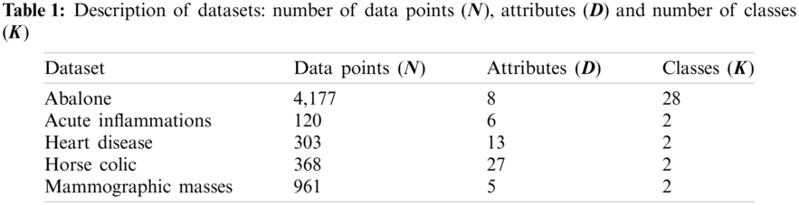
Five benchmark datasets obtained from the UCI repository [41] are included in this investigation, with Tab. 1 giving their details. Abalone consists of 4,177 instances, where eight physical measurements are used to divide these data into 28 age groups of abalone. There is only one categorical attribute, while the rest are continuous. Acute Inflammations was originally created by a medical expert to assess the decision support system, which performs the presumptive diagnosis of two diseases of urinary system: acute inflammations of urinary bladder and acute nephritises [42]. There are 120 instances, each representing a potential patient with six symptom attributes (1 numerical and 5 categorical). Heart Disease contains 303 records of patients collected from Cleveland Clinic Foundation. Each data record is described by 13 attributes (5 numerical and 8 nominal) regarding heart disease diagnosis. This dataset is divided into two classes referring to the presence and absence of heart disease in the examined patients. Horse Colic has 368 data records of injured horses, each of which is described by 27 attributes (7 numerical and 19 nominal). These collected instances are categorized into two classes: ‘Yes’ indicating that lesion is surgical and ‘No’ otherwise. About 30% of the original are missing values. For simplicity, missing nominal values in this dataset are equally treated as a new nominal value. In the case of missing numerical values, mean of the corresponding attribute is used. Mammographic Masses contains mammogram data of 961 patient records collected at the Institute of Radiology of the University Erlangen-Nuremberg between 2003 and 2006. Five attributes used to describe each record are BI-RADS assessment, age and three BI-RADS attributes. This dataset possesses two class labels referring to the severity of a mammographic mass lesion: benign (516 instances) and malignant (445 instances).

4.2 Experimental Design

This experiment aims to examine the quality of the LCEWCT and LCEWTQ extensions of LCE for clustering mixed numeric and nominal data. For these extended models where k-prototypes is used for creating a cluster ensemble, the parameter γ of this base clustering algorithm is randomly selected from {0.1,0.2,…,5}. The results with LCE models are compared against a large number of standard clustering techniques and advanced cluster ensemble approaches. At first, this includes three standard clustering algorithms: k-prototypes, k-centers, k-means (KM) and dSqueezer. Particularly, the weight parameter γ is randomly selected from {0.1,0.2,…,5} for each run of k-prototypes and k-centers. In order to exploit k-means, a mixed-type dataset needs to be pre-processed such that each nominal attribute is transformed to β new binary-value features, where β is the corresponding number of nominal values. For the case of dSqueezer, each numerical data attribute has to be mapped to the corresponding categorical domain using the discretisation method explained by [19]. The set of compared methods also contains twelve different cluster ensemble techniques that have been reported in the literature for their effectiveness in combining clustering results: four graph-based methods of HBGF [28], CSPA [32], HGPA [32] and MCLA [32]; two pairwise-similarity based methods [24] of EAC-SL and EAC-AL; and six feature-based methods of IVC [43], MM [33], QMI [33], AGGF [29], AGGLSF [29] and AGGLSR [29]. The experiment setting employed in this evaluation is exhibited below. Note that the performance of standard clustering algorithms is always assessed over the original data, without using any information of cluster ensembles.

•   Cluster ensemble methods are investigated using four different ensemble types: Full-space + Fixed-k, Full-space + Random-k, Subspace + Fixed-k, and Sub-space + Random-k.

•   Ensemble size (M) of 10 base clusterings is experimented.

•   As in [24,28,29], each method divides data points into a partition of K (the number of true classes for each dataset) clusters, which is then evaluated against the corresponding true partition. Note that, true classes are known for all datasets but are not explicitly used by the cluster ensemble process. They are only used to evaluate the quality of the clustering results.

•   The quality of each cluster ensemble method with respect to a specific ensemble setting is generalized as the average of 50 runs. Based on the central limit theorem (CLT), the observed statistics in a controlled experiment can be justified to the normal distribution [43].

•   The constant decay factor (DC) of 0.9 is exploited with WCT and WTQ algorithms.

4.3 Performance Measurements and Comparison

Provided that the external class labels are available for all experimented datasets, the results of final clustering are evaluated using the validity index of Normalized Mutual Information (NMI) introduced by [32]. Other quality measures such as Classification Accuracy (CA; [44]) and Adjusted Rand Index (AR; [45]) can be similarly used. However, unlike other criteria, NMI is not biased by a large number of clusters, thus providing a reliable conclusion. This also simplifies the magnitude of evaluation results and their comprehension. This quality index measures the average mutual information (i.e., the degree of agreement) between two data partitions. One is obtained from a clustering algorithm (π∗) while the other is taken from a priori information, i.e., known class labels (∏′). With NMI∈[0,1], the maximum value indicates that the clustering result and the original classes completely match. Given the two data partitions of K clusters and K′ classes, NMI is computed by the following equation.

NMI(π∗,∏′)=∑i=1K⁡∑j=1K′⁡ni,jlog⁡(ni,jNnimj)∑i=1K⁡nilog⁡(niN)∑j=1K′⁡mjlog⁡(mjN),(12)

where ni,j is the number of data objects agreed by cluster i and class j, ni is the number of data objects in cluster i, mj is the number of data objects in class j and N is the total number of data objects. To compare the performance of different cluster ensemble methods, the overall quality measure for a specific experiment setting (i.e., dataset and ensemble type) is obtained as the average of NMI values across 50 trials. These method-specific means may be used for the comparison purpose only to a certain extent. To achieve a more reliable assessment, the number of times (or frequencies) that one technique is ‘significantly better’ and ‘significantly worse’ (of 95% confidence level) than the others are considered here. This comparison method has been successfully exploited by [9] and [46] to discover trustworthy conclusions from the results generated by different cluster ensemble approaches. Based on these, it is useful to compare the frequencies of better (B) and worse (W) performance between methods. The overall measure (B−W) is also used as a summarization.

4.4 Experimental Results

Fig. 4 shows the overall performance of different clustering methods, as the average NMI measure across all investigated datasets and ensemble types. Based on this, LCEWCT and LCEWTQ are similarly more effective than their baseline model (i.e., HBGF), whilst significantly improve the quality of data partitions acquired by base clusterings, i.e., k-prototypes. Their performance levels are also better than other cluster ensemble methods and standard clustering algorithms included in this evaluation. Note that CSPA and k-means are the most accurate amongst the aforementioned two groups of compared methods. In addition, feature-based approaches such as QMI and IVC are unfortunately incapable of enhancing the accuracy of base clustering results. Dataset-specific results are given in Tabs. A to E of Supplementary (https://drive.google.com/file/d/1I62X5LTDQ_u6feFx57tW9oqwDLtfu4eH/view?usp=sharing).

Figure 4: performance of different clustering methods, averaged across five datasets and four ensemble types. Note that each error bar represents the standard deviation of the corresponding average

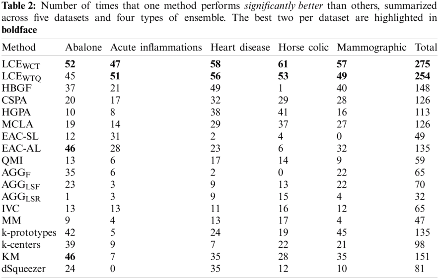
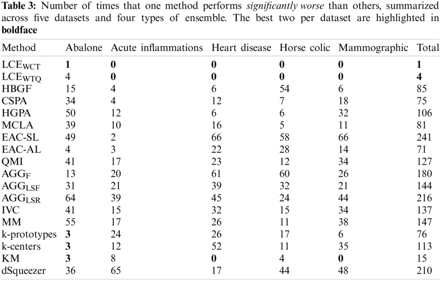
To further evaluate the quality of identified techniques, the number of times (or frequency) that one method is significantly better and worse (of 95% confidence level) than the others are assessed across all experimented datasets and ensemble types. Tabs. 2 and 3 present for each method the frequencies of significant better (B) and significant worse (W) performance, respectively. According to the frequencies shown in Tab. 2, LCEWCT and LCEWTQ perform equally well on most of the examined datasets. EAC-AL is exceptionally effective on ‘Abalone’ data, while the three graph-based approaches of CSPA, HGPA and MCLA are of good quality with ‘Heart Disease’ and ‘Horse Colic’. Note that k-means and k-prototypes are the best amongst basic clustering techniques. It is also interesting to see that the better-performance statistics of feature-based approaches are usually lower than those of standard clusterings considered here. These findings can be similarly observed in Tab. 3, which illustrates the frequencies of worse performance (W). In this specific evaluation context, k-means is notably effective for most datasets and outperforms many graph-based and pairwise-similarity based cluster ensemble methods.

Besides, the relations between performance of experimented cluster ensemble methods with respect to different ensemble types are also examined for this experiment: Full-space + Fixed-k, Full-space + Random-k, Subspace + Fixed-k, and Subspace + Random-k. Specifically, Fig. 5 shows the average NMI measures of different approaches across datasets. According to this statistical illustration, LCEWCT and LCEWTQ are more effective than other techniques across different ensemble types, with their best performance being obtained with ‘Subspace + Fixed-k’. HBGF and three graph-based approaches (CSPA, HGPA and MCLA) are also more effective on Subspace ensemble types, as compared to the Full-space alternatives. While both ‘Fixed-k’ and ‘Random-k’ strategies equally lead to good performance of link-based techniques, feature-based and pair-wise similarity based methods perform better using the latter.

Figure 5: Performance of clustering methods, categorized by four ensemble types

The quality of LCEWCT and LCEWTQ with respect to the perturbation of DC and M parameters is also studied for the clustering of mixed-type data. Fig. 6 presents the relation between different values of DC∈{0.1,…,0.9} and the quality of data partitions generated by both LCE methods – the average NMI measure across all ensemble types, where M is fixed to 10 for comparison simplicity. In general, the performance of LCEWCT and LCEWTQ gradually improve as the value of DC increases. Another parameter to be assessed is the ensemble size (M). Fig. 7 shows the association between the performance of various techniques and different values of M∈{10,20,…,100}. Both LCE methods perform consistently better than their baseline model competitors across different ensemble sizes, where the decay factor (DC) is fixed to 0.9 for simplicity. Their performance levels also incline with the increasing ensemble size.

Figure 6: Relations between DC∈{0.1,0.2,…,0.9} and performance of LCE methods (averages of NMI over four ensemble types for each dataset). Measure of HBGF is also included for a comparison

Figure 7: Relations between M ∈ {10, 20, …, 100} and performance of LCE methods (presented as the averages of NMI over four ensemble types for each dataset)

5  Conclusion

This paper has presented the novel extension of link-based consensus clustering to mixed-type data analysis. The resulting models have been rigorously evaluated on benchmark datasets, using several ensemble types. The comparison results against different standard clustering algorithms and a large set of well-known cluster ensemble methods show that the link-based techniques usually provide solutions of higher quality than those obtained by competitors. Furthermore, the investigation of their behavior with respect to the perturbation of algorithmic parameters also suggests the robust performance. Such a characteristic makes link-based cluster ensembles highly useful for the exploration and analysis of a new set of mixed-type data, where prior knowledge is minimal. Because of its scope, there are many possibilities for extending the current research. Firstly, other link-based similarity measures may be explored. As more information within a link network is exploited, link-based cluster ensembles are likely to be more accurate (see the relevant findings in the initial work [30,31], where the use of SimRank and its variants is examined). However, it is important to note that such modification is more resource intensive and less accurate in a noisy environment than the present setting. Secondly, performance of link-based cluster ensembles may be further improved using an adaptive decay factor (DC), which is determined from the dataset under examination.

The diversity of cluster ensembles has a positive effect on the performance of the link-based approach. It is interesting to observe the behavior of the proposed models to new ensemble generation strategies, e.g., the random forest method for clustering [47], which may impose a higher diversity amongst base clusterings. Another non-trivial topic is related to the determination of ensemble components’ significance. This discrimination or selection process usually leads to a better outcome. The coupling of such a mechanism with the link-based cluster ensembles is to be further studied. Despite its performance, the consensus function of spectral graph partitioning (SPEC) can be inefficient with a large RA matrix. This can be overcome through the approximation of eigenvectors required by SPEC. As a result, the time complexity becomes linear to the matrix size, but with possible information loss. A better alternative has been introduced by [48] via the notion of Power Iteration Clustering (PIC). It does not actually find eigenvectors but discovers interesting instances of their combinations. As a result, it is very fast and has proven more effective than the conventional SPEC. The application of PIC as a consensus function of link-based cluster ensembles is a crucial step towards making the proposed approach truly effective in terms of run-time and quality. Other possible future works include the use of proposed method to support accurate clusterings for fuzzy reasoning [49], handling of data with missing values [50] and data discretization [51].

Acknowledgement: This research work is partly supported by Mae Fah Luang University and Newton Institutional Links 2020-21 project (British Council and National Research Council of Thailand).

Funding Statement: This work is funded by Newton Institutional Links 2020–21 project: 623718881, jointly by British Council and National Research Council of Thailand (https://www.britishcouncil.org). The first author is the project PI with the other participating as a Co-I.

Conflicts of Interest: There is no conflict of interest to report regarding the present study.

References

 1.  D. Jiang, C. Tang and A. Zhang, “Cluster analysis for gene expression data: A survey,” IEEE Transactions on Knowledge and Data Engineering, vol. 16, no. 11, pp. 1370–1386, 2004. [Google Scholar]

 2.  R. Wu, R. Chen, C. Chang and J. Chen, “Data mining application in customer relationship management of credit card business,” in Proc. of Int. Conf. on Computer Software and Applications, Edinburgh, UK, pp. 39–40, 2005. [Google Scholar]

 3.  J. Zhang, J. Mostafa and H. Tripathy, “Information retrieval by semantic analysis and visualization of the concept space of D-lib magazine,” D-Lib Magazine, vol. 8, no. 10, pp. 1–8, 2002. [Google Scholar]

 4.  J. Costa and M. Netto, “Cluster analysis using self-organizing maps and image processing techniques,” in Proc. of IEEE Int. Conf. on systems, Man, and Cybernetics, vol. 5, pp. 367–372, 1999. [Google Scholar]

 5.  Q. He, J. Wang, Y. Zhang, Y. Tang and Y. Zhang, “Cluster analysis on symptoms and signs of traditional Chinese medicine in 815 patients with unstable angina,” in Proc. of Int. Conf. on Fuzzy Systems and Knowledge Discovery, Tianjin, China, pp. 435–439, 2009. [Google Scholar]

 6.  A. K. Jain, R. Duin and J. Mao, “Statistical pattern recognition: A review,” IEEE Transactions on Pattern Analysis and Machine Intelligence, vol. 22, no. 1, pp. 4–37, 2000. [Google Scholar]

 7.  D. B. Henry, P. H. Tolan and D. Gorman-Smith, “Cluster analysis in family psychology research,” Journal of Family Psychology, vol. 19, no. 1, pp. 121–132, 2005. [Google Scholar]

 8.  K. Kim and H. Ahn, “A recommender system using GA K-means clustering in an online shopping market,” Expert Systems with Applications, vol. 34, pp. 1200–1209, 2008. [Google Scholar]

 9.  N. Iam-On, T. Boongoen and S. Garrett, “LCE: A link-based cluster ensemble method for improved gene expression data analysis,” Bioinformatics, vol. 26, no. 12, pp. 1513–1519, 2010. [Google Scholar]

10. E. Kim, S. Kim, D. Ashlock and D. Nam, “MULTI-K: Accurate classification of microarray subtypes using ensemble k-means clustering,” BMC Bioinformatics, vol. 10, no. 260, pp. 1–12, 2009. [Google Scholar]

11. A. K. Jain, M. Murty and P. Flynn, “Data clustering: A review,” ACM Computing Survey, vol. 31, no. 3, pp. 264–323, 1999. [Google Scholar]

12. Z. Huang, “Clustering large data sets with mixed numeric and categorical values,” in Proc. of Pacific Asia Conf. on Knowledge Discovery and Data Mining, Singapore, pp. 21–34, 1997. [Google Scholar]

13. S. Dudoit and J. Fridyand, “A prediction-based resampling method for estimating the number of clusters in a dataset,” Genome Biology, vol. 3, no. 7, pp. 1–21, 2002. [Google Scholar]

14. T. Boongoen and Q. Shen, “Nearest-neighbor guided evaluation of data reliability and its applications,” IEEE Transactions on Systems, Man and Cybernetics, Part B, vol. 40, no. 6, pp. 1622–1633, 2010. [Google Scholar]

15. W. M. Rand, “Objective criteria for the evaluation of clustering methods,” Journal of the American Statistical Association, vol. 66, pp. 846–850, 1971. [Google Scholar]

16. A. Ahmad and L. Dey, “A k-mean clustering algorithm for mixed numeric and categorical data,” Data and Knowledge Engineering, vol. 63, no. 2, pp. 503–527, 2007. [Google Scholar]

17. N. Iam-On, T. Boongoen, S. Garrett and C. Price, “Link-based cluster ensembles for heterogeneous biological data analysis,” in Proc. of IEEE Int. Conf. on Bioinformatics and Biomedicine, pp. 573–578, 2010. [Google Scholar]

18. H. A. Ralambondrainy, “Conceptual version of the k-means algorithm,” Pattern Recognition Letters, vol. 16, pp. 1147–1157, 1995. [Google Scholar]

19. Z. He, X. Xu and S. Deng, “Scalable algorithms for clustering large datasets with mixed type attributes,” International Journal of Intelligent Systems, vol. 20, pp. 1077–1089, 2005. [Google Scholar]

20. Z. He, X. Xu and S. Deng, “Squeezer: An efficient algorithm for clustering categorical data,” Journal of Computer Science and Technology, vol. 17, no. 5, pp. 611–624, 2002. [Google Scholar]

21. Z. Huang, “Extensions to the k-means algorithm for clustering large data sets with categorical values,” Data Mining and Knowledge Discovery, vol. 2, pp. 283–304, 1998. [Google Scholar]

22. W. Zhao, W. Dai and C. Tang, “K-centers algorithm for clustering mixed type data,” in Proc. of Pacific-Asia Conf. on Advances in Knowledge Discovery and Data Mining, Nanjing, China, pp. 1140–1147, 2007. [Google Scholar]

23. R. Duda, P. Hart and D. Stork, “Unsupervised learning and clustering,” Pattern Classification, 2nd ed., Singapore: Wiley-Interscience, 2000. [Google Scholar]

24. A. Fred and A. K. Jain, “Combining multiple clusterings using evidence accumulation,” IEEE Transaction on Pattern Analysis and Machine Intelligence, vol. 27, no. 6, pp. 835–850, 2005. [Google Scholar]

25. H. Xue, S. Chen and Q. Yang, “Discriminatively regularized least-squares classification,” Pattern Recognition, vol. 42, no. 1, pp. 93–104, 2009. [Google Scholar]

26. N. Iam-On, T. Boongoen, S. Garrett and C. Price, “A link-based approach to the cluster ensemble problem,” IEEE Transactions on Pattern Analysis and Machine Intelligence, vol. 33, no. 12, pp. 2396–2409, 2011. [Google Scholar]

27. N. Iam-On and T. Boongoen, “Pairwise similarity for cluster ensemble problem: Link-based and approximate approaches,” Springer Transactions on Large-Scale Data and Knowledge-Centered Systems, vol. 9, pp. 95–122, 2013. [Google Scholar]

28. X. Z. Fern and C. E. Brodley, “Solving cluster ensemble problems by bipartite graph partitioning,” in Proc. of Int. Conf. on Machine Learning, Louisville, Kentucky, USA, pp. 36–43, 2004. [Google Scholar]

29. A. Gionis, H. Mannila and P. Tsaparas, “Clustering aggregation,” ACM Transactions on Knowledge Discovery from Data, vol. 1, no. 1, pp. 4–ex, 2007. [Google Scholar]

30. N. Iam-On, T. Boongoen and S. Garrett, “Refining pairwise similarity matrix for cluster ensemble problem with cluster relations,” in Proc. of Int. Conf. on Discovery Science, Budapest, Hungary, pp. 222–233, 2008. [Google Scholar]

31. N. Iam-On and S. Garrett, “Linkclue: A MATLAB package for link-based cluster ensembles,” Journal of Statistical Software, vol. 36, no. 9, pp. 1–36, 2010. [Google Scholar]

32. A. Strehl and J. Ghosh, “Cluster ensembles: A knowledge reuse framework for combining multiple partitions,” Journal of Machine Learning Research, vol. 3, pp. 583–617, 2002. [Google Scholar]

33. A. Topchy, A. K. Jain and W. Punch, “Clustering ensembles: Models of consensus and weak partitions,” IEEE Transaction on Pattern Analysis and Machine Intelligence, vol. 27, no. 12, pp. 1866–1881, 2005. [Google Scholar]

34. N. Iam-On and T. Boongoen, “Diversity-driven generation of link-based cluster ensemble and application to data classification,” Expert Systems with Applications, vol. 42, no. 21, pp. 8259–8273, 2015. [Google Scholar]

35. P. Panwong, T. Boongoen and N. Iam-On, “Improving consensus clustering with noise-induced ensemble generation,” Expert Systems with Applications, vol. 146, pp. 113–138, 2020. [Google Scholar]

36. H. Luo, F. Kong and Y. Li, “Clustering mixed data based on evidence accumulation,” in Proc. of Int. Conf. on Advanced Data Mining and Applications, Xian, China, pp. 348–355, 2006. [Google Scholar]

37. M. Smolkin and D. Ghosh, “Cluster stability scores for microarray data in cancer studies,” BMC Bioinformatics, vol. 21, no. 9, pp. 1927–1934, 2003. [Google Scholar]

38. Z. Yu, H. Wong and H. Wang, “Graph-based consensus clustering for class discovery from gene expression data,” Bioinformatics, vol. 23, no. 21, pp. 2888–2896, 2007. [Google Scholar]

39. L. Adamic and E. Adar, “Friends & neighbors on the web,” Social Networks, vol. 25, no. 3, pp. 211–230, 2003. [Google Scholar]

40. A. Ng, M. Jordan and Y. Weiss, “On spectral clustering: Analysis and an algorithm,” Advances in Neural Information Processing Systems, vol. 14, pp. 849–856, 2001. [Google Scholar]

41. A. Asuncion and D. Newman, "UCI machine learning repository," https://archive.ics.uci.edu, 2007. [Google Scholar]

42. J. Czerniak and H. Zarzycki, “Application of rough sets in the presumptive diagnosis of urinary system diseases,” in Proc. of Int. Conf. on AI and Security in Computing Systems, Miedzyzdroje, Poland, pp. 41–51, 2003. [Google Scholar]

43. H. Tijms, “Understanding Probability: Chance Rules in Everyday Life,” Cambridge, UK: Cambridge University Press, 2004. [Google Scholar]

44. N. Nguyen and R. Caruana, “Consensus clusterings,” in Proc. of IEEE Int. Conf. on Data Mining, Omaha, Nebraska, USA, pp. 607–612, 2007. [Google Scholar]

45. L. Hubert and P. Arabie, “Comparing partitions,” Journal of Classification, vol. 2, no. 1, pp. 193–218, 1985. [Google Scholar]

46. L. I. Kuncheva, “Experimental comparison of cluster ensemble methods,” in Proc. of Int. Conf. on Fusion, Florence, Italy, pp. 105–115, 2006. [Google Scholar]

47. T. Shi and S. Horvath, “Unsupervised learning with random forest predictors,” Journal of Computational and Graphical Statistics, vol. 15, no. 1, pp. 118–138, 2006. [Google Scholar]

48. F. Lin and W. Cohen, “Power iteration clustering,” in Proc. of Int. Conf. on Machine Learning, Haifa, Israel, pp. 655–662, 2010. [Google Scholar]

49. X. Fu, T. Boongoen and Q. Shen, “Evidence directed generation of plausible crime scenarios with identity resolution,” Applied Artificial Intelligence, vol. 24, no. 4, pp. 253–276, 2010. [Google Scholar]

50. M. Pattanodom, N. Iam-On and T. Boongoen, “Clustering data with the presence of missing values by ensemble approach,” in Proc. of Asian Conf. on Defence Technology, Chiang Mai, Thailand, pp. 151–156, 2016. [Google Scholar]

51. K. Sriwanna, T. Boongoen and N. Iam-On, “Graph clustering-based discretization of splitting and merging methods,” Human-centric Computing and Information Sciences, vol. 7, no. 1, pp. 1–39, 2017. [Google Scholar]

This work is licensed under a Creative Commons Attribution 4.0 International License, which permits unrestricted use, distribution, and reproduction in any medium, provided the original work is properly cited.