Computers, Materials & Continua DOI:10.32604/cmc.2022.018423
Article

Image Segmentation Based on Block Level and Hybrid Directional Local Extrema

Ghanshyam Raghuwanshi1, Yogesh Gupta2, Deepak Sinwar1, Dilbag Singh3, Usman Tariq4, Muhammad Attique5, Kuntha Pin6 and Yunyoung Nam7,*

1Manipal University Jaipur, Jaipur, 302026, India
2BML Munjal University, Gurugram, India
3Bennett University, Greater Noida, India
4College of Computer Engineering and Sciences, Prince Sattam Bin Abdulaziz University, Al-Khraj, Saudi Arabia
5Department of Computer Science, HITEC University Taxila, Taxila, Pakistan
6Department of ICT Convergence, Soonchunhyang University, Asan 31538, Korea
7Department of Computer Science and Engineering, Soonchunhyang University, Asan, Korea
*Corresponding Author: Yunyoung Nam. Email: ynam@sch.ac.kr
Received: 08 March 2021; Accepted: 05 May 2021

Abstract: In the recent decade, the digitalization of various tasks has added great flexibility to human lifestyle and has changed daily routine activities of communities. Image segmentation is a key step in digitalization. Segmentation plays a key role in almost all areas of image processing, and various approaches have been proposed for image segmentation. In this paper, a novel approach is proposed for image segmentation using a nonuniform adaptive strategy. Region-based image segmentation along with a directional binary pattern generated a better segmented image. An adaptive mask of 8 × 8 was circulated over the pixels whose bit value was 1 in the generated directional binary pattern. Segmentation was performed in three phases: first, an image was divided into sub-images or image chunks; next, the image patches were taken as input, and an adaptive threshold was generated; and finally the image chunks were processed separately by convolving the adaptive mask on the image chunks. Gradient and Laplacian of Gaussian algorithms along with directional extrema patterns provided a double check for boundary pixels. The proposed approach was tested on chunks of varying sizes, and after multiple iterations, it was found that a block size of 8 × 8 performs better than other chunks or block sizes. The accuracy of the segmentation technique was measured in terms of the count of ill regions, which were extracted after the segmentation process.

Keywords: Image segmentation; HDEP; block-level processing; adaptive threshold

1  Introduction

Image segmentation is the key stage and works as a vital step for many image-processing applications [1]. In an image segmentation process, an image is divided into uniform or homogeneous regions, and these regions can be decided by some common attributes such as the position of image pixels, color properties, patterns, and shape features [2]. Human perception of image geometry or object identification and the gap in understanding the system can be minimized using proper image segmentation. Filling this semantic gap remains the most difficult challenge, and therefore it has been deeply analyzed and investigated in recent years [3]. An image can be composed of different types of intensity values. An image can be categorized into background and foreground regions based on the intensity values. Image analysis can be more effective when using image segmentation techniques. Previously, various approaches have been introduced for segmenting an image into meaningful areas called objects [4,5]. Segmentation techniques are categorized into two types: similarity-based and discontinuity-based segmentation. Segmentation plays a key role in almost all areas such as image retrieval, object identification, medical image processing [6,7], image de-noising, and remote sensing image processing [8,9]. Recently, deep learning [10,11] and constrained based image segmentation were proposed for improving image segmentation [12]. Images, in general, have richer contents, and the area of interest in images cannot be determined accurately without a proper image segmentation technique. To achieve a perfect image analysis i.e., to better identify the target, it is critical to filter out unwanted content from the image [13]. Image segmentation can be done using image features such as texture, homogeneity, and intensity value of a pixel. Foreground intensity pixels refer to the specific region or target of interests in the image. To extract these target areas from the image, proper segmentation techniques are required. Sometimes the object can be of lighter intensities, whereas the background pixels are of higher intensities, leading to inaccurately segmented regions [14]. This issue can be resolved by adopting a dynamic or adaptive thresholding technique, as well as by processing the image at a block or region-level. Each block can be processed independently using its own threshold. At a later stage, adjacent blocks or regions can be merged based on their block or region properties or boundary value analysis. Region growing and merging is also one of the most widely used approaches for image segmentation. The basic idea behind this approach is to start with the initial properties of the block or the seed value provided by a user [15]. Various approaches have been published to date for improving results [16] using the region growing and merging approach [17,18]. After image segmentation, the results are evaluated based on some parameters. More importantly, the next stage can only be started if an image is segmented by a more optimal segmentation technique. There are two ways to segment an image either at a region or block level or at a global level. A globally extracted threshold may not justify the image geometry perfectly and requires a deeper analysis of image geometry before calculating the threshold value [19]. The global threshold can be used to divide an image into two regions: foreground (object) and background. However, if the image has richer contents or more than one object, the global threshold will not work. However, local analysis will be fruitful if the image has richer content. If multiple objects are there within the image boundary along with the background, then multiple thresholds are required at different blocks, which is referred to as local threshold processing for each block [20,21].

Processing the entire image at one level is not a good idea because there may be blocks or parts that do not contribute significantly to the definition of the object or content. Moreover, these regions may be considered ill or noncontributing regions. Segmentation is one method for identifying and removing noncontributing parts of an image to make it more meaningful, and it serves as an input for subsequent processing stages. To achieve better feature extraction, proper image segmentation is critical; otherwise, improper segmentation may result in information loss and have a negative impact on the feature extraction process.

1.1 Threshold Calculation

Image thresholding is an important preprocessing step [22]. There are three ways to calculate the threshold of an image. The first approach follows the threshold calculation at a global or image level. In this approach, a collective decision is taken regarding the threshold value, and the same calculated threshold value is applied to complete the image. It is easier to calculate and can benefit images with homogeneous pixel values or image intensities that are nearly identical, such as texture images. The formula for calculating the global threshold is as follows:

g(x,y)={1if(x,y)>T0if(x,y)≤T}(1)

The global threshold approach assumes that the histogram must be bimodal. Hence, the extraction of the contributing objects can be performed by creating a threshold boundary between the background pixels and objects, as shown in Fig. 1.

Figure 1: Separation of background pixels from the objects based on (a) Local threshold (b) global threshold

The resultant thresholded image will be a binary image, where 0 and 1 represent the pixel values. The pixel value 1 denotes objects, whereas 0 denotes background regions. However, it suffers from the problem of not considering the local geometry or local intensity of the image; hence, this approach is unable to justify the procedure at the local level; in the case of heterogeneous content, this approach degrades the performance of image segmentation. Local thresholding is another approach that considers local image geometry by considering each pixel value in the threshold calculation process. Usually, the pixel value indicated by 0 represents white, whereas 255 represents black. However, pixel values between 1 and 254 represent different intensity levels. This technique works better than the global thresholding method because it allows images to have different intensity (contrast) levels. Various thresholding approaches have been reported to date for image thresholding. The assumption for local thresholding is that small patches of images are most suitable for a similar intensity illumination, which results in an almost uniform pixel distribution. Dividing images into patches is the first preprocessing step of image segmentation for local thresholding, and then the optimal threshold for each image patch is calculated by investigating its histogram. The threshold calculation for each pixel is performed by interpolating the results of all sub-image patches. The only issue with this approach is its computational cost; therefore, it is not suitable for applications where time is of the essence, such as real-time image processing applications.

1.2 Motivation

The proposed method addresses the issues and limitations of existing segmentation techniques and proposes a solution for existing issues in the following manner.

The global thresholding approach results in injustice with the local geometry of the image, which is resolved by providing a novel adaptive thresholding technique at the regional level.

The gradient and Laplacian of Gaussian algorithms cannot perfectly justify image boundaries. Two-stage verification of the boundary pixels is required for a better analysis of the boundary regions. The proposed method includes two-fold verification of boundary pixels, in which the Laplacian of Gaussian is used in the first fold and the Extrema Pattern is used in four directions in the second fold.

The correlation of the local properties of the image patch with the global properties of the image must be done correctly. The proposed method addresses these issues by establishing a proper relationship between the local intensity values and the global intensity of the entire image.

A nonuniform adaptive approach should be followed for acquiring segments of variable sizes. The proposed method adds a variable threshold that maintains the adaptive behavior for each image patch and behaves according to the local image geometry.

2  Proposed Method

The proposed method segments the image using a nonuniform and adaptive approach. As a preprocessing step, the proposed method first divides the image into non-overlapping sub-blocks. Each block is treated as a separate image or block, and each block is processed separately. Instead of global thresholding, a local thresholding approach was considered for individual blocks. Local image geometry can be handled better by including the adaptive threshold, as well as by considering the local intensity values when processing the adaptive threshold.

2.1 Adaptive Threshold Calculation

The proposed method considers the local thresholding of an image. At the initial stage, the local intensity contribution at each block is calculated by analyzing the relationships among the intensity values within an image patch of 8 × 8. Generally, most of the information remain in the central part of the image; however, boundary pixels may also contribute to selecting the edges of objects or segments. Each pixel contributes to the threshold calculation process. Hereafter, boundary pixels can be considered by padding the pixel values at the boundary areas of the image.

Threshold calculation is done as follows:

T[x,y,f(x,y),p(x,y)]=f(x,y)∗max(block)min(block)+average(block)(2)

Here, x and y are the coordinates in the horizontal and vertical directions, f (x, y) is the location of the pixel, and p (x, y) is the intensity value at the location. As shown in Eq. (2), the proposed method prepares an adaptive mask by placing the calculated threshold value at the corresponding location in the generated mask. The generated adaptive mask is illustrated in Fig. 2.

Threshold values are related to the geometry of the local block. According to the formula given in Eq. (2), if the minimum pixel values and average pixel values are the same, the region is a texture region or a region with homogenous pixel values. According to the object detection rule, abrupt changes in the intensity value and the collection of heterogeneous pixel intensity values are the primary sources for the possibility of finding objects in those areas. The proposed image segmentation system is shown in Fig. 3, and the working procedure of the proposed method is presented in Tab. 1.

Figure 2: Adaptive mask at block-level

Figure 3: Proposed image segmentation system

2.2 Non-Uniform Segmentation

The proposed approach sub-divides the image into non-overlapping regions. However, the separation of adjacent regions may produce faulty segments if the adjacent regions have similar properties. Uniform segmentation does not deal with the faulty segments, and a segmented image will have more ill objects. To alleviate this issue, the proposed approach follows the non-uniform segmentation technique. The proposed method for achieving non-uniform segmentation is as follows:

Input: Region of the image

Output: Non-uniform region (after merging)

Step 1: for i = 1 to number_of_region

Step 2: if (gradient (i)<=Threshold)

goto step 3

then

calculate Laplacian of region(i);

else

goto Step 4.

Step 3: Repeat the same process as done in Step 2 for next adjacent regions.

Step 4: Check the Laplacian(i) with the Laplacian(i+1) [i.e., of next adjacent region]

If((Laplacian(i)-Laplacian(i+1)||Laplacian(i)-Laplacian(2i)||Laplacian(i)-Laplacian(2i+1))<β)

then

merge the regions with region(i)

Step 5: Non-uniform regions

However, the first step in both uniform and non-uniform segmentation is the same, that is, both divide the image into non-overlapping regions. In uniform segmentation, by default, all segments are of the same size, and the decision to consider the segment is based on parameters such as homogeneity, intensity distribution, and percentage of object existence within the segment. However, the proposed segmentation technique is based on a nonuniform segmentation approach. The proposed approach considers the gradient descent and Laplacian of Gaussian for calculating the segment boundary, as explained in the algorithm presented in Tab. 1. The proposed method captures the adaptive behavior of the filter and manages the non-uniformity of the segment. A proper segment does not bind to any specific size, and it can vary according to the image properties.

Image decomposition results in different chunks of specific sizes as shown in Fig. 4. Each chunk is classified into a specific category based on its placement in the original image, such as at the top, bottom, or middle. Furthermore, these categories were further divided into three categories, as shown in Fig. 4. The association of these chunks into specific categories is done to determine the boundary value of the chunks with their neighboring chunks. However, each chunk will be compared along with the boundary pixels with the neighboring pixels. There are certain angles on which comparison is done as shown in Fig. 6. Meanwhile, if the neighboring chunks meet the desired criteria, only merging can be done. Boundary pixels are shown in different colors in Fig. 6, from which it can be understood that certain boundary pixels will be overlapped (at the corners of the chunk) each time. This overlapping will help decide whether a boundary pixel is belonging to more than one chunk.

Figure 4: Different categories of partitioned areas of image. (a) Top left chunk; (b) Top middle chunk; (c) Top right chunk; (d) Middle left chunk, and (e) Angles at different degrees

2.3 Effect of Block Size and Mask Size

The proposed approach considers chunks of different sizes. However, the size of each block did not reflect the size of the mask. Blocks of smaller sizes result in the presence of ill objects in the segmented image, as shown in Fig. 5. Another effect of small chunks is that more merging steps are required in every phase. The proposed method iterates through the different images on the chunks of different sizes, and after executing multiple iterations, it is concluded that an 8 × 8 block size is more suitable for the segmentation process. However, Fig. 5 shows that the number of ill objects is smaller in the blocks of 16 × 16 and 32 × 32 sizes, but the performance of adaptive mask decreases as the size of each block is increased from 8 × 8. The performance of the adaptive mask decreases with an increase in the block size because it takes the local maximum intensity value in the threshold generation process. If the size of the mask is larger, it creates an adverse effect on the adaptive mask calculation because the radius of the local geometry will be increased; the local maximum intensity value may not be able to justify with the complete image patch.

Figure 5: Relation of block size and ill (faulty) objects

Figure 6: Boundary pixels (in colors) for comparisons with neighboring regions

Block-level processing of an image is an important aspect of the proposed image segmentation system. Block-level processing reduces the number of pixels in the pattern generation phase and simultaneously increases the discriminative power. Small blocks lead to more information loss, whereas larger blocks result in less discriminative power. Fig. 5 shows that blocks of smaller sizes result in more information loss.

2.4 Extrema Pattern Calculation

The extrema pattern determines the boundary value of any pixel in different directions. According to the placement of the image chunk or patch, the weight difference extrema pattern can be calculated as follows: The WD-EP was calculated using D1=IPa−IPcand D2=IPc−IPb.

EP(α)={0if((IPc>IPa&&IPc<IPb)or(IPc⟨IPa&&IPc⟩IPb))1elseifD1≥ϕD2≥ϕ0else}(4)

EP=∑p=1BL⁡{Kα(gc);Kα(g1);Kα(g2);…Kα(g8)}(5)

where α={0∘,90∘,180∘,270∘}, BL is the number of image chunks or patches, and K(gi) is the resultant difference (either 0 or 1) between the neighboring pixels and the current central pixel in the specified α direction. ϕ is the user-specified threshold. IPa, IPb, and IPc are the pixel values to be compared. Eq. (5) shows that if there is no edge in the generated pattern, the bit having value “0” will not change in EP. However, if there is an edge (i.e., the DLEP pattern has a bit value “1”), the bit value will be checked against the threshold and set to “0 s” if it does not satisfy the threshold condition.

The proposed method deals well with segments of irregular sizes by thoroughly investigating the boundary pixels with their neighboring pixels in the four principal directions (90°, 180°, 0°, and 270°). Eventually, the generated binary pattern determines whether the boundary pixels have relations with their adjacent neighboring pixels of another block. This will be decided in the following way:

EPα={Trueif(count_of_1bit{Kα(gc);Kα(g1);Kα(g2);…Kα(g8)})>6Falseothrwise} (6)

Here, EPα is the generated extrema pattern in the specific direction α (i.e.,0∘,90∘,180∘,270∘). count_of_1bit is a function that counts the occurrence of “1-bit” values in the generated pattern. The size of the pattern is nine bits long, and the above equation shows that if the total number of 1-bit values is more than six, then only will it be considered the boundary pixel, which is related to the neighboring block. There is a significant value of not only the count of 1-bit value but also the position of the pixel values in the generated pattern. A similar process of binary pattern generation is initiated from the neighboring block. If the count_of_1bitfunction returns “True,” both neighboring blocks will be merged; otherwise, they will be processed separately with their respective segments. The process of extreme pattern calculation minimizes the effect of ill or false segments from the generated results, as shown in Fig. 7.

Each boundary pixel was compared with the adjacent pixels in the 90° direction. It is shown in Fig. 8 that the generated pattern has 7 “1-bit” values. The proposed method sets the threshold of six for merging blocks; hence, adjacent blocks are merged in this case.

Figure 7: Effect of block size on information loss (unused pixels)

Figure 8: Extrema pattern (EP) for α = 900 and pattern = 011111011

2.5 Experimental Result and Discussion

The proposed method was tested on images from the COREL 1k dataset. The image segmentation process was performed on images with heterogeneous content because the resultant segmented image contains regions of similar or homogeneous content. There were 10 categories in the COREL dataset. Representative images of the COREL dataset are presented in Fig. 9.

Figure 9: Example images from COREL database for image segmentation. (a) Image with boat; (b) Image with humans; (c) Image with human in a sea and boats, and (d) Humans running in a water

The efficiency of the image segmentation technique was determined by counting the number of ill or noncontributing regions. Faulty segments were extracted after segmentation if the segmented image contained more ill regions, resulting in faulty segments. Fig. 10 shows the resultant segmented reasons based on certain threshold values. The proposed method sets the area of the segment as a threshold; therefore, segmented regions with areas greater than 250 were considered and those with less than 250 were discarded.

Figure 10: (a–d): Extracted segments, indicated in red are selected against the area threshold

The proposed method achieves better image segmentation by considering the local image geometry analysis of the images, as shown in Fig. 11. The segmented images at various stages are shown in Fig. 11. Fig. 11a shows the background of the image based on the adaptive threshold. Fig. 11b shows the image after subtracting it from the background, and Fig. 11c shows the final segmented image after applying the mask of 8 × 8. From Fig. 12, it is observed that meaningful objects can be extracted by minimizing the effect of the ill segments or regions in the segmented image. However, the nonuniform and adaptive threshold selection approach also significantly and collectively works together to achieve a better segmented image. The area threshold works well to achieve the segmented image, and segmented regions are extracted separately based on the calculated adaptive threshold, as shown in Fig. 12.

Figure 11: Image segmentation at different phases. (a) Adaptive thresholding; (b) Image subtraction; (c) Final image; (d) Refinement

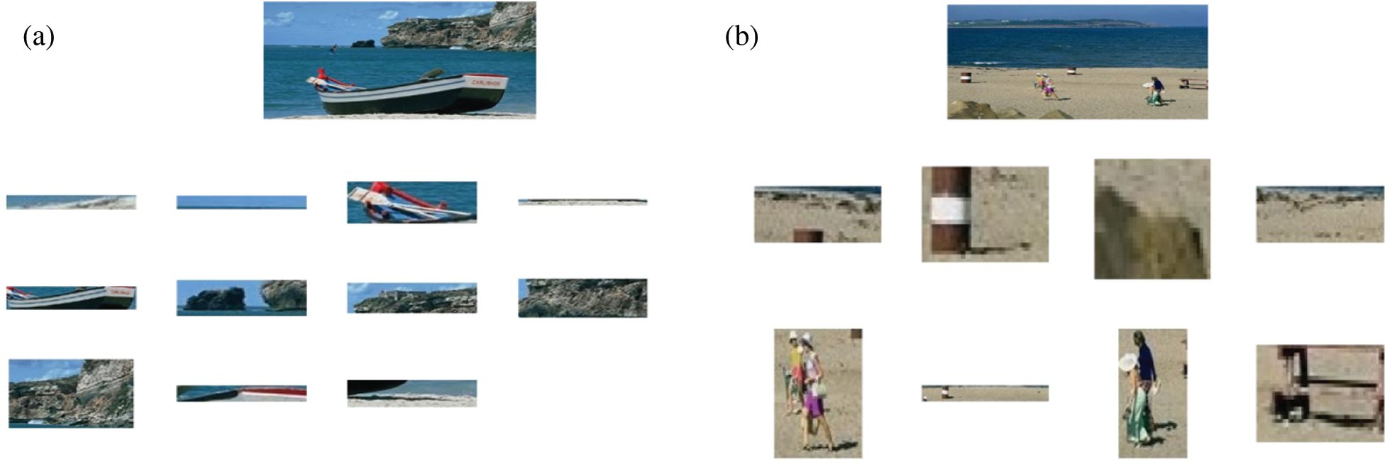
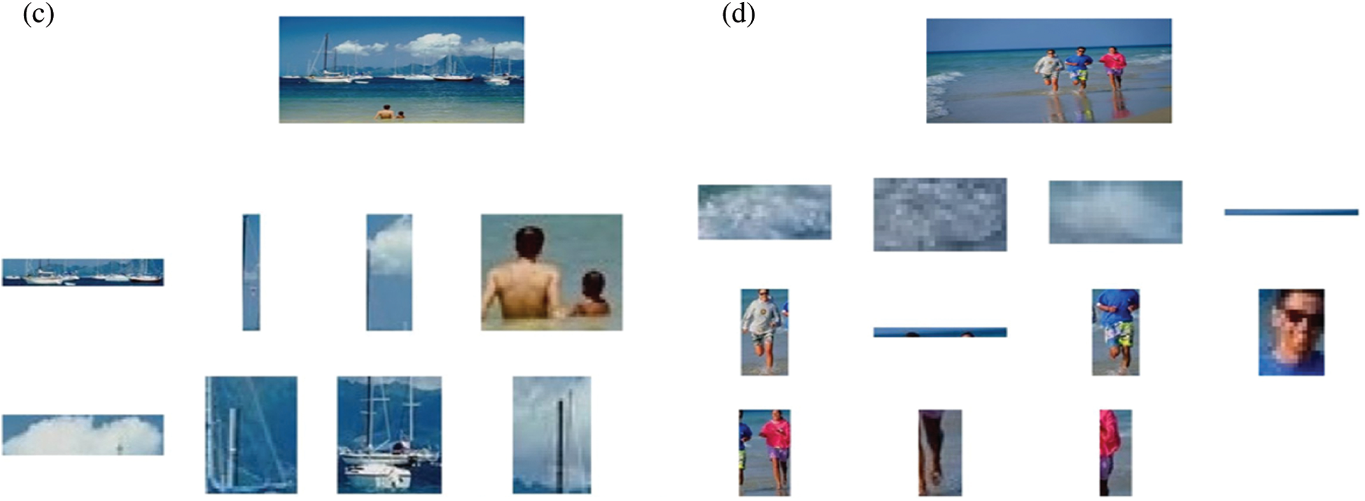
Figure 12: Extracted segments from the original image. (a–d) Meaningful segmented objects with the reference of Fig. 9

3  Conclusion

The proposed method presents a system for digital image segmentation using Novel Extrema Pattern and Laplacian of Gaussian. Image analysis is done at block or region level by dividing the image into non-overlapping sub images or regions. The proper boundary analysis among the adjacent blocks is done by the proposed extrema pattern. Adaptive threshold is the another key feature of the proposed method which works as an input for the variable mask. Adaptive Threshold is calculated by the local properties of the local image patch and global properties of the image. Generate variable mask convolves over the image block and results in better image segmentation. The proposed segmentation system performs well with the images of dense diversity due to region level analysis. The Proposed method tested the accuracy of the segmentation on the heterogeneous images which are taken from the COREL dataset. However, proposed system works well with the images of homogeneous contents too. The experimental results show that the proposed segmentation method out-performs on the block size of 8 × 8 with better segmentation accuracy. The proposed method can be further extended in future for image retrieval purposes and critical analysis of the medical images.

Funding Statement: This research was supported by the MSIT (Ministry of Science and ICT), Korea, under the ICAN (ICT Challenge and Advanced Network of HRD) program (IITP-2021-2020-0-01832) supervised by the IITP (Institute of Information & Communications Technology Planning & Evaluation) and the Soonchunhyang University Research Fund.

Conflicts of Interest: The authors declare that they have no conflicts of interest to report regarding the present study.

This work is licensed under a Creative Commons Attribution 4.0 International License, which permits unrestricted use, distribution, and reproduction in any medium, provided the original work is properly cited.