Computers, Materials & Continua DOI:10.32604/cmc.2022.019447
Article

VISPNN: VGG-Inspired Stochastic Pooling Neural Network

Shui-Hua Wang1, Muhammad Attique Khan2 and Yu-Dong Zhang3,*

1School of Mathematics and Actuarial Science, University of Leicester, Leicester, LE1 7RH, United Kingdom
2Department of Computer Science, HITEC University Taxila, Taxila, 47080, Pakistan
3School of Informatics, University of Leicester, Leicester, LE1 7RH, United Kingdom
*Correspondence Author: Yu-Dong Zhang. Email: yudongzhang@ieee.org
Received: 14 April 2021; Accepted: 28 June 2021

Abstract: Aim Alcoholism is a disease that a patient becomes dependent or addicted to alcohol. This paper aims to design a novel artificial intelligence model that can recognize alcoholism more accurately. Methods We propose the VGG-Inspired stochastic pooling neural network (VISPNN) model based on three components: (i) a VGG-inspired mainstay network, (ii) the stochastic pooling technique, which aims to outperform traditional max pooling and average pooling, and (iii) an improved 20-way data augmentation (Gaussian noise, salt-and-pepper noise, speckle noise, Poisson noise, horizontal shear, vertical shear, rotation, Gamma correction, random translation, and scaling on both raw image and its horizontally mirrored image). In addition, two networks (Net-I and Net-II) are proposed in ablation studies. Net-I is based on VISPNN by replacing stochastic pooling with ordinary max pooling. Net-II removes the 20-way data augmentation. Results The results by ten runs of 10-fold cross-validation show that our VISPNN model gains a sensitivity of 97.98 ± 1.32, a specificity of 97.80 ± 1.35, a precision of 97.78 ± 1.35, an accuracy of 97.89 ± 1.11, an F1 score of 97.87 ± 1.12, an MCC of 95.79 ± 2.22, an FMI of 97.88 ± 1.12, and an AUC of 0.9849, respectively. Conclusion The performance of our VISPNN model is better than two internal networks (Net-I and Net-II) and ten state-of-the-art alcoholism recognition methods.

Keywords: Deep learning; alcoholism; multiple-way data augmentation; VGG; convolutional neural network; stochastic pooling

1  Introduction

Alcoholism (also known as alcohol use disorder) is a disease that a patient becomes dependent or addicted to alcohol [1]. Patients with alcoholism continue to drink alcohol; even drinking causes negative consequences to themselves. The difference between alcoholism and alcohol abuse is people of alcohol abuse are not physically dependent on alcohol [2]. Excessive alcohol use will damage all organ systems, but it mainly influences the heart, liver, brain, pancreas, and immune system [3]. Besides, alcoholism may cause schizophrenia, bipolar disorder, depression [4], irregular heartbeat [5], Wernicke–Korsakoff syndrome [6], etc.

Long-term alcoholism affects the brain, i.e., the volumes of white matter and grey matter of patients are smaller than age-matched controls. The brain shrinkages and lateral ventricle enlargement [7] caused by alcoholism can be observed via magnetic resonance imaging (MRI) scanning, which facilitates doctors diagnosing alcoholism.

Nevertheless, the diagnosis of alcoholism is mainly based on manual observation of brain images in the current clinical routine, which is naturally labor-intensive and onerous. Mainly, the slight shrinkage of alcoholism brains in the early prodromal stage [8] associated with mild symptoms is susceptible to be neglected by radiologists and clinicians, which may trigger costs to the patient and his/her family. In light of the above limitations, accurate and fast diagnostic artificial intelligence (AI) models to recognize alcoholism are beneficial to patients, families, and society.

In the past, various AI models have been proposed to recognize alcoholism. Fig. 1 shows the relationship between AI with machine learning (ML) and deep learning (DL). ML is a subfield of AI, while DL is a subfield of ML. Hou [9] brought about a novel algorithm—Predator-prey Adaptive-inertia Chaotic Particle Swarm Optimization (PACPSO). The authors applied the PACPSO to identify alcoholism. Jenitta et al. [10] presented a local mesh vector co-occurrence pattern (LMVCoP) feature for assisting diagnosis. This method can be used for the application of alcoholism identification. Han [11] proposed a three-segmented encoded Jaya (3SJ) method to identify alcoholism. The authors found the 3SJ gave better performance than other optimization methods, such as multi-objective genetic algorithm, plain Jaya, bee colony optimization, particle swarm optimization, etc. Lima [12] presented a novel method utilizing Haar wavelet transform (HWT) to extract features from brain scanning images of patients. Their method achieved an accuracy of 81.57 ± 2.18% on their dataset. Afterward, Macdonald [13] presented a wavelet energy logistic regression (WELR) model. The authors used 5-fold stratified cross-validation to verify the performances of their model. Qian [14] proposed a computer vision-based technique that utilizes cat swarm optimization (CSO), which mimics the behaviour of the cats. In their experiment, CSO was demonstrated to have better performances than four bio-inspired algorithms. Chen [15] presented a new model combining support vector machine (SVM) with genetic algorithm (GA). The combined model is abbreviated as SVMGA. The authors stated their model was effective in alcoholism detection, showing an average accuracy of 88.68 ± 0.30%. Chen [16] presented an AI model based on a linear regression classifier (LRC) for alcoholism detection.

Recently, DL techniques have been successfully applied to alcoholism recognition. Lv [17] created a 7-layer convolutional neural network (CNN). Their experiments showed stochastic pooling (SP) provided better performance than other pooling methods. Nevertheless, their CNN structure was simple, so its expression ability was limited. Xie [18] used the AlexNet transfer learning (ANTL) model. The authors fine-tuned their model and tested five different replacement configurations.

There are some other ML methods based on different data sources. For example, Kamarajan et al. [19] used random forest and Electroencephalogram (EEG) source functional connectivity, neuropsychological functioning, and impulsivity measures to classify alcohol use disorder. Quaglieri et al. [20] harnessed functional MRI (fMRI) to analyze brain network underlying executive functions in gambling and alcohol use disorder. Many other scanning modalities and protocols may help identify alcoholism; however, we focus on MRI in this study due to its high-resolution three-dimensional imaging ability.

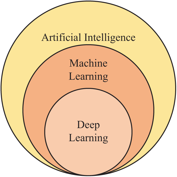
Figure 1: Relationship among AI, ML, and DL

The motivation of this paper is to propose a novel model, VGG-inspired stochastic pooling neural network (VISPNN), for alcoholism recognition with an expectation to obtain better performance than existing alcoholism identification approaches. The contributions of our study are the following four aspects.

(a)   A VGG-inspired network is used as a mainstay network.

(b)   Stochastic pooling is used to replace traditional max pooling.

(c)   Improved multiple-way data augmentation is proposed to avoid overfitting.

(d)   Our model is proven to render better performances than state-of-the-art methods.

2  Methodology

2.1 Introduction of VGG

Tab. 1 displays the abbreviation list in this study for ease of reading. First, we introduce VGG, which stands for Visual Geometry Group, an academic group at Oxford University. The VGG team presented two renowned networks: VGG-16 [21] and VGG-19, encompassed as library packages of prevalent programming language platforms, e.g., Python and MATLAB.

Fig. 2 displays the structure of VGG-16, which is composed of five convolutional blocks (CBs) and three fully connected layers (FCLs). The size of the input of VGG-16 is 224×224×3. After the 1st CB, the output is 112×112×64. Components of 1st CB are shown in Tab. 2. The 1st CB can be written as

a×(bc×c)/d (1)

which means “a repetitions of b kernels with sizes of c×c followed by a max-pooling with a size of d×d.”

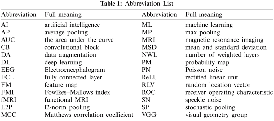
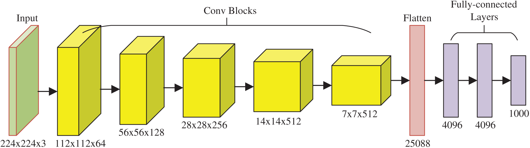
Figure 2: Diagram of VGG-16 network structures

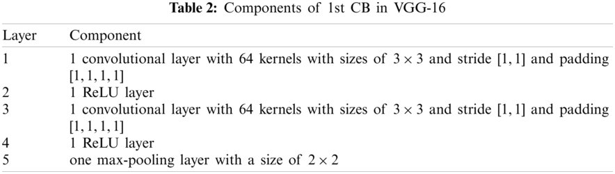
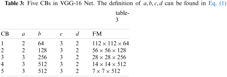
Note that (i) the activation function: rectified linear unit (ReLU) layers are skipped in the subsequent texts as default. (ii) Stride and padding are not reported because they can be calculated easily. The five CBs are itemized in Tab. 3, and the feature map (FM) of the output is displayed in the final column. After five CBs, the FM is compressed from 7×7×512 to a vector with a size of 25,088 neurons. Three FCLs with neurons of 4096, 4096, and 1000 are appended at last.

2.2 Improvement I: Stochastic Pooling

Within the standard CNNs, pooling is an essential component followed by a convolution layer (See Layer 5 in Tab. 2) to reduce the size of FMs. Traditional pooling methods are either max-pooling (MP) or average pooling (AP).

Suppose we have an FM, which can be separated into M1×M2 blocks, in which every block has the size of Q1×Q2. Now let us focus on the m1-th row and m2-th column block

Bm1,m2={b(x,y),x=1,⋯,Q1,y=1,⋯,Q2}. (2)

where 1≤m1≤M1,1≤m2≤M2 (See Fig. 3).

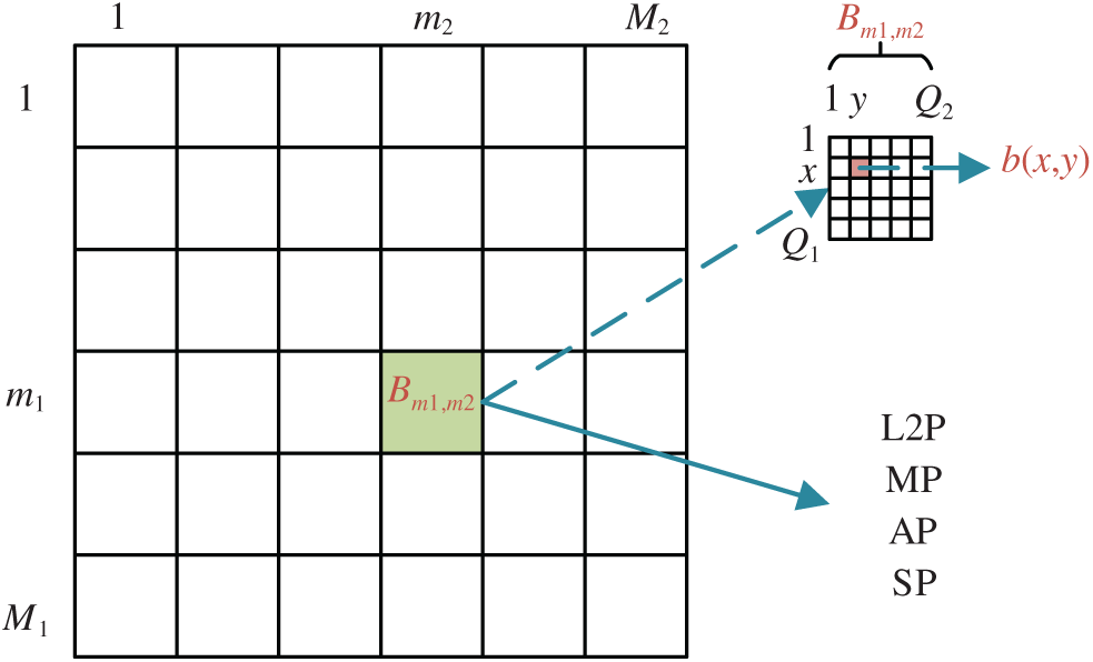
Figure 3: Diagram of block-wise processing

The strided convolution (SC) traverses the input activation map with the strides, which equals the size of the block (Q1,Q2), so here its output is set to

Bm1,m2SC=b(1,1). (3)

The l2-norm pooling (L2P), average pooling (AP), and max pooling (MP) generate the l2-norm value, average value, and maximum value within the block Bm1,m2, respectively. Nevertheless, the AP outputs the average, downscaling the greatest values, where the essential features may lie. In contrast, MP stores the most significant value but deteriorates the overfitting obstacle.

{Bm1,m2L2P=∑x=1Q1∑y=1Q2b2(x,y)Q1×Q2Bm1,m2AP=1Q1×Q2∑x=1Q1∑y=1Q2b(x,y)Bm1,m2MP=maxx=1Q1maxy=1Q2b(x,y) (4)

Alternatively, stochastic pooling (SP) provides a way to the defects of AP and MP. Successful application cases are using SP in the stochastic resonance model [22], COVID-19 recognition [23], etc. SP is a four-step procedure. Step 1 generates the probability map (PM) for each entry in the block Bm1,m2.

{S(x,y)=b(x,y)∑x=1Q1∑y=1Q2b(x,y)s.t.∑x=1Q1∑y=1Q2S(x,y)=1 (5)

where S(x,y) stands for the PM value at pixel (x,y).

Step 2 creates a random location vector (RLV) r=(xr,yr) that takes the discrete probability distribution (DPD) as

{Z[r=(1,1)]=S(1,1)Z[r=(1,2)]=S(1,2)⋯Z[r=(1,Q2)]=S(1,Q2)Z[r=(2,1)]=S(2,1)Z[r=(2,2)]=S(2,2)⋯Z[r=(2,Q2)]=S(2,Q2)⋯⋯⋯⋯Z[r=(Q1,1)]=S(Q1,1)Z[r=(Q1,2)]=S(Q1,2)⋯Z[r=(Q1,Q2)]=S(Q1,Q2) (6)

where Z represents the probability.

Step 3, a sample location vector r0 is drawn from the RLV r, and we have r0=(xr0,yr0).

Step 4, the output of SP is at location r0, namely

Bm1,m2SP=b(xr0,yr0) (7)

Fig. 4 gives an example where we can observe the 1-st row and 2-nd column block B12, outlined by red rectangle. The L2P calculates

B1,2L2P=∑(6.42+7.32+6.42+9.52+5.72+0.52+3.62+1.12+7.82)9=6.08 (8)

The AP and MP output the pooling values of 5.37 and 9.5, respectively. In contrast, the SP generates the PM and selects the top-left pixel b(1,1)=0.13 in the block B12 and output the SP value of 6.4.

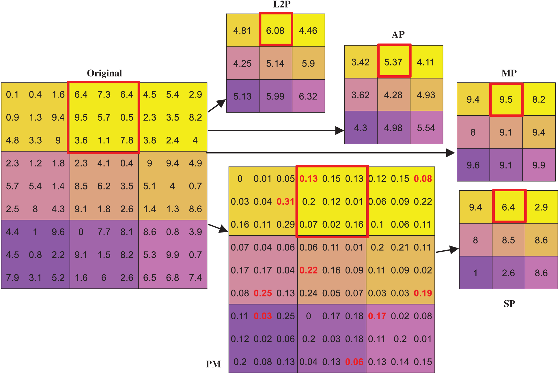
Figure 4: Comparison of different pooling methods

2.3 Improvement 2: VGG-Inspired Stochastic Pooling Neural Network

A novel VGG-inspired mainstay network is proposed. Tab. 4 shows the structure of the proposed 10-layer VGG-inspired mainstay network. The definition of (a,b,c,d) can be found in Tabs. 2 and 3. The variables (e,f) represents the weights and biases of FCL, respectively. The NWL in Tab. 4 represents the number of weighted layers. The total weighted layers in this VGG-inspired mainstay network is 1+2+3+2+1+1=10. We can observe that after four CBs, the size of output FM is 11×11×64, which is flattened to a vector of 7744, which is then sent through an FCL with 100 neurons, finally outputting two neurons indicating alcoholism or healthy.

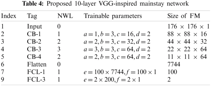
The structure of our VGG-inspired mainstay network is displayed in Fig. 5a. If we replace the max-pooling in each CB with stochastic pooling, we can get the proposed VGG-Inspired Stochastic Pooling Neural Network (VISPNN), as shown in Fig. 5b.

2.4 Improvement 3: 20-Way Data Augmentation

The dataset in this study was reported in Ref. [18], composed of 188 alcoholic brain images and 191 non-alcoholic brain images. Fig. 6 shows two samples of our dataset.

The relatively small dataset may breed the overfitting problem. To avoid this, data augmentation (DA) is a powerful tool because it can generate fake images on the training set. Cheng [23] presented a 16-way DA, in which 8 DA techniques were applied on both q(k) and q(h)(k). The multiple-way DA shows better performance than traditional DA. This study is based on 16-way DA from Cheng [23]; furthermore, we add two new DAs on both q(k) and q(h)(k). One DA is speckle noise (SN), which alters the image as

qSN(k)=q(k)+NSN×q(k) (9)

where NSN is uniformly distributed random noise. The mean and variance of NSN are set to 0 and 0.05, respectively.

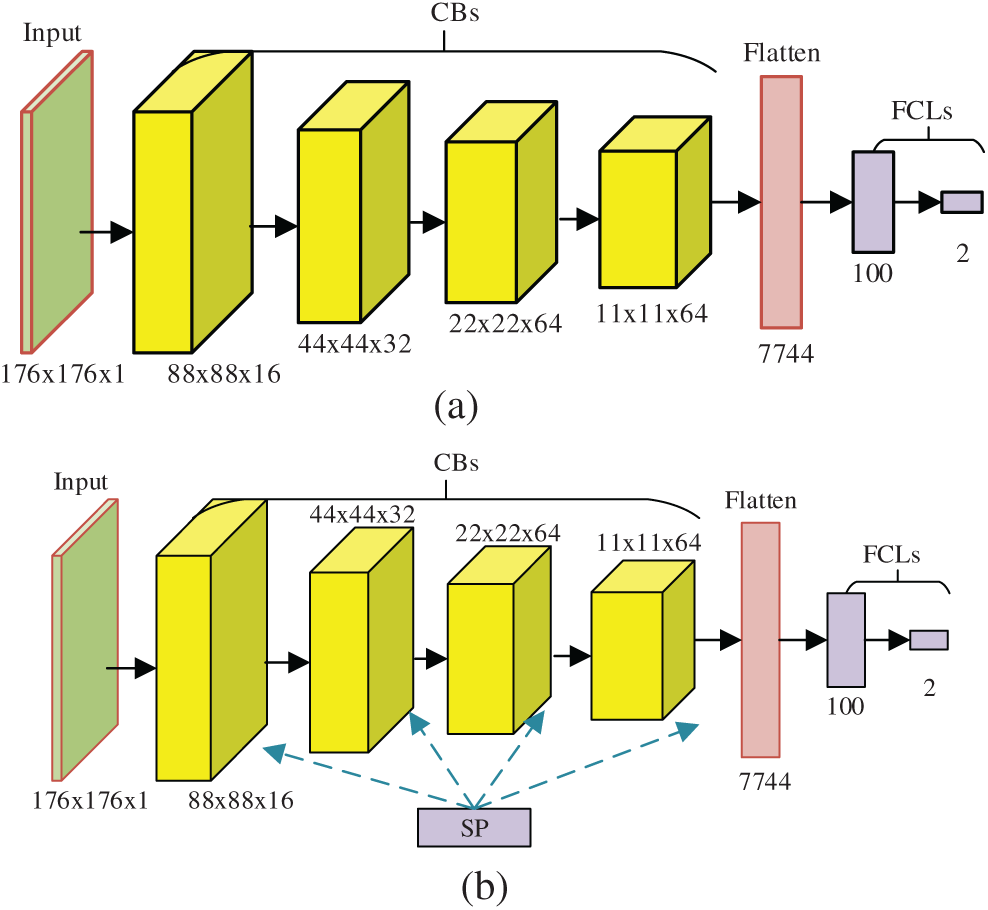
Figure 5: Diagram of two proposed networks (a) VGG-inspired mainstay network (b) proposed VISPNN

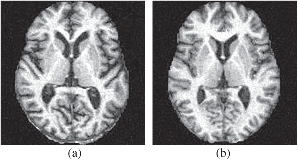
Figure 6: Samples of our dataset (a) alcoholism and (b) HC

The other DA is Poisson noise (PN). In the electronics field, PN originates from the discrete nature of the electric charge. Instead of adding artificial noise to the raw image, we generate PN from the raw image. The pixel values of raw images are stored in uint 8 format; if a pixel has the value of 20, then the corresponding pixel qPN of the PN altered image will be generated from a Poisson distribution with a mean of 20. Mathematically

{qt(k∣x,y)∼Po[q(k∣x,y)]qPN(k∣x,y)=min{256,qt(k∣x,y)} (10)

where Po(λ) represents a Poisson distribution with a mean of λ, and (x,y) are the coordinates. qt is the temporary variable. The min function helps the final output is within the value of [0,256]. Using a colourful natural image can observe how those two noises alter the image, as shown in Fig. 7.

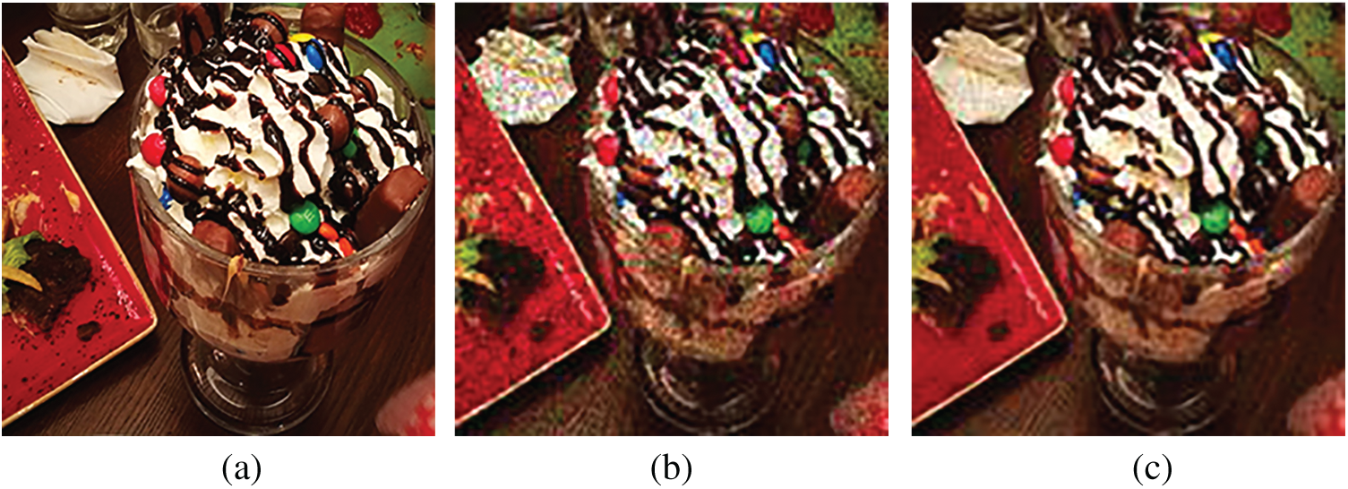
Figure 7: Raw image and its altered images by two new Das (a) raw image q(k), (b) SN altered qSN(k) and (c) PN altered qPN(k)

With the help of SN and PN, we can propose a novel 20-way DA, First, M1 different DA methods as shown in Fig. 8 are applied to q(k). Let Km,m=1,…,M1 be each DA operation, we have M1 augmented datasets on raw image q(k) as:

Km[q(k)],m=1,…,M1. (11)

Let M2 stand for the size of generated new images for each DA method, we have

|Km[q(k)]|=M2. (12)

Second, horizontally mirrored image is generated as:

q(h)(k)=ya[q(k)] (13)

where ya stands for horizontal mirror function.

Third, all the M1 different DA methods are performed on the mirrored image q(h)(k). We generate M1 new datasets as:

{Km[q(h)(k)],m=1,⋯,M1|Km[q(h)(k)]|=M2,m=1,…,M1 (14)

Fourth, the raw image q(k), the mirrored image q(h)(k), all the above M1-way results of raw image Km[q(k)], and all M1-way DA results of horizontal mirrored image Km[q(h)(k)] are combined. The final generated dataset from q(k) is defined as G(k):

q(k)↦G(k)=yb{q(k)q(h)(k)K1[q(k)]⏟M2K1[q(h)(k)]⏟M2⋯⋯KM1[q(k)]⏟M2KM1[q(h)(k)]⏟M2} (15)

where yb stands for the concatenation function. Suppose augmentation factor is M3, which stands for the number of images in G(k), we obtain

M3=|G(k)||q(k)|=(1+M1×M2)×21=2×M1×M2+2 (16)

Algorithm 1 summarizes the pseudocode of the proposed 20-way DA method. In this study, we set M1=10, i.e., a 20-way DA. We also set M2=30, thus M3=602, indicating each raw training image will generate 602 images, including the raw image itself.

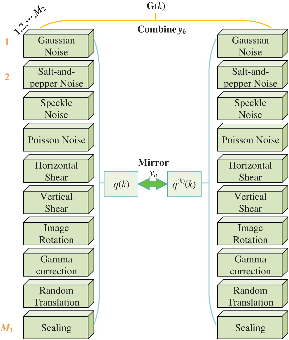
Figure 8: Diagram of proposed 20-way DA

2.5 Implementation

R-fold cross-validation is employed. The whole dataset is divided into R folds [24]. At r-th trial, 1≤r≤R, the r-th fold is picked up as the test, and the rest R−1 folds: [1,…,r−1,r+1,…,R] are chosen as training set (Fig. 9). We let R=10, namely a 10-fold cross validation. Furthermore, we run the 10-fold cross validation ten times.

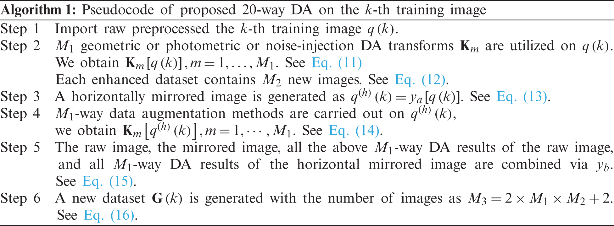
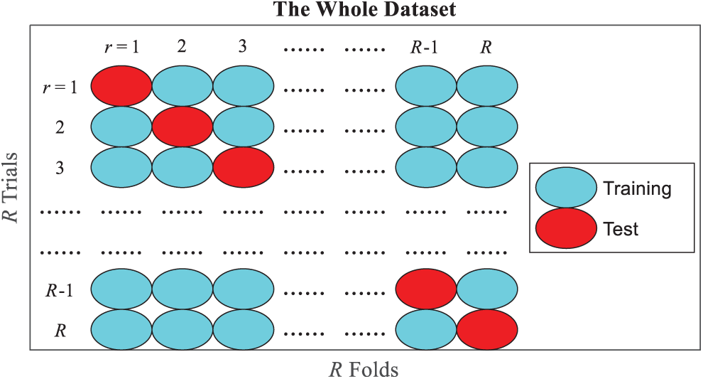
Figure 9: Diagram of R-fold cross validation

2.6 Measures

Seven measures are used based on the confusion matrix of 10 runs of 10-fold cross-validation. Let I stands for the confusion matrix

I=[I(1,1)I(1,2)I(2,1)I(2,2)] (17)

where I(1,1) means true positive, I(1,2) false negative (FN), I(2,1) false positive, and I(2,2) true negative. Sensitivity, specificity, precision, and accuracy are already familiarized to readers, so we will not give their definitions. Besides, we use the F1 score, Matthews correlation coefficient (MCC), and Fowlkes–Mallows index (FMI).

F1=2I(1,1)2I(1,1)+I(2,1)+I(1,2), (18)

MCC=I(1,1)×I(2,2)−I(2,1)×I(1,2)(I(1,1)+I(2,1))×(I(1,1)+I(1,2))×(I(2,2)+I(2,1))×(I(2,2)+I(1,2)), (19)

FMI=I(1,1)I(1,1)+I(2,1)×I(1,1)I(1,1)+I(1,2), (20)

The receiver operating characteristic (ROC) curve is used to provide a graphical plot of measuring AI models. First, the ROC curve is produced by plotting the true positive rate against the false-positive rate at various threshold levels. Then, the area under the curve (AUC) is calculated via ROC.

3  Results

3.1 20-Way DA Results

Fig. 10 shows the M1-way DA results of raw image, which is chosen as Fig. 6a. Due to the page limit, we do not display the horizontally mirrored image and the corresponding M1-way DA results.

3.2 Statistical Results of Proposed Method

Tab. 5 itemizes the statistical results (10 runs of 10-fold cross-validation) of the proposed VISPNN method. The mean and standard deviation (MSD) over ten runs are displayed in the last row. It shows our model reaches a sensitivity of 97.98 ± 1.32, a specificity of 97.80 ± 1.35, an accuracy of 97.89 ± 1.11, respectively.

3.3 Ablation Studies

An ablation study is a procedural experiment that removes a network's submodule to understand that submodule better. Two ablation studies are carried out: (i) Net-I: We remove stochastic pooling from the proposed VISPNN model and use max-pooling to replace the removed layers. Thus, the network is named Net-I. (ii) Net-II: We remove the multiple-way data augmentation. The resultant network is named Net-II. The comparison of our VISPNN model with Net-I and Net-II is shown in Tab. 6.

Fig. 11 displays the ROC curves comparison of the proposed VISPNN model with Net-I and Net-II. The blue patches correspond to the lower and upper confidence bounds. The AUC of Net-I is 0.9683, compared to that of VISPNN of 0.9849. Therefore, we can observe stochastic pooling indeed increase performances. Meanwhile, the AUC of Net-II is 0.9602, which is a significant drop from VISPNN (0.9849). This drop reflects that multiple-way data augmentation can significantly increase the prediction performance due to its ability to generate diverse ``fake'' training images.

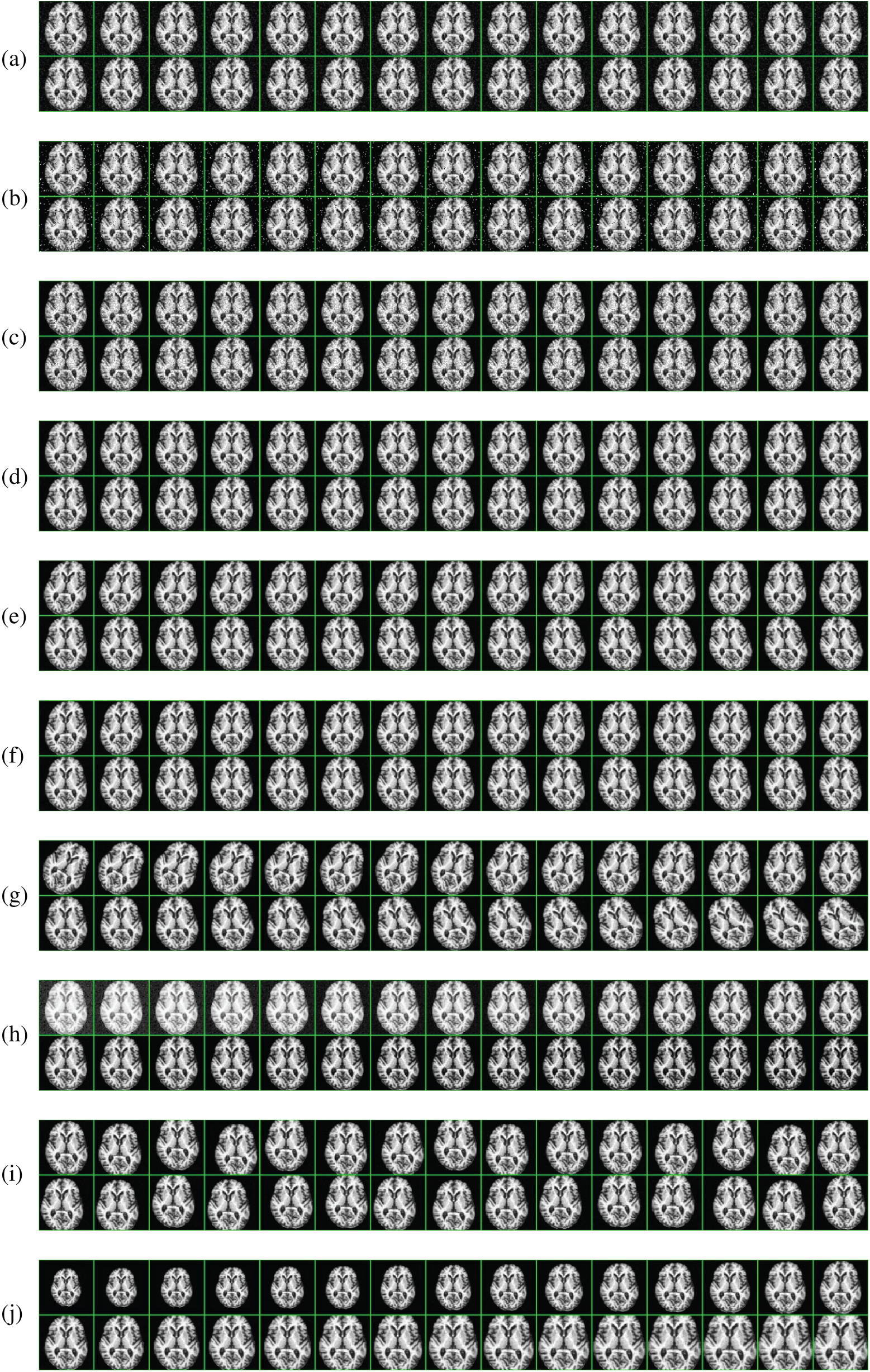
Figure 10: 20-way DA results (we only show 10-way DA results on the raw image here). (a) Gaussian noise (b) Salt-and-pepper noise (c) Speckle noise (d) Poisson noise (e) Horizontal shear (f) Vertical shear (g) Image rotation (h) Gamma correction (i) Random translation (j) Scaling

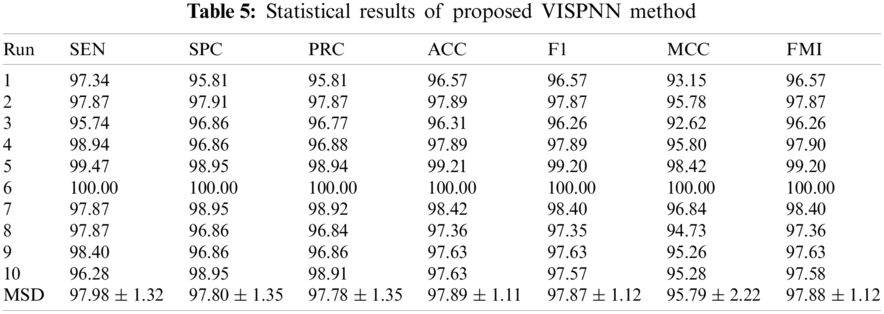
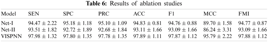
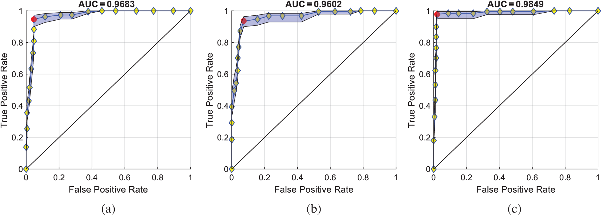
Figure 11: ROC comparison of ablation studies (a) Net-I, (b) Net-II and (c) VISPNN

3.4 Comparison to Other Alcoholism Recognition Methods

This proposed VISPNN model is compared with 10 state-of-the-art alcoholism recognition methods: PACPSO [9], LMVCoP [10], WRE [11], HWT [12], WELR [13], CSO [14], SVMGA [15], LRC [16], CNNSP [17], and ANTL [18], respectively. The comparison results are itemized in Tab. 7, with the cognate bar plot shown in Fig. 12 which ranks all the methods in order of MCC.

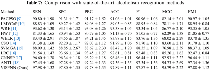
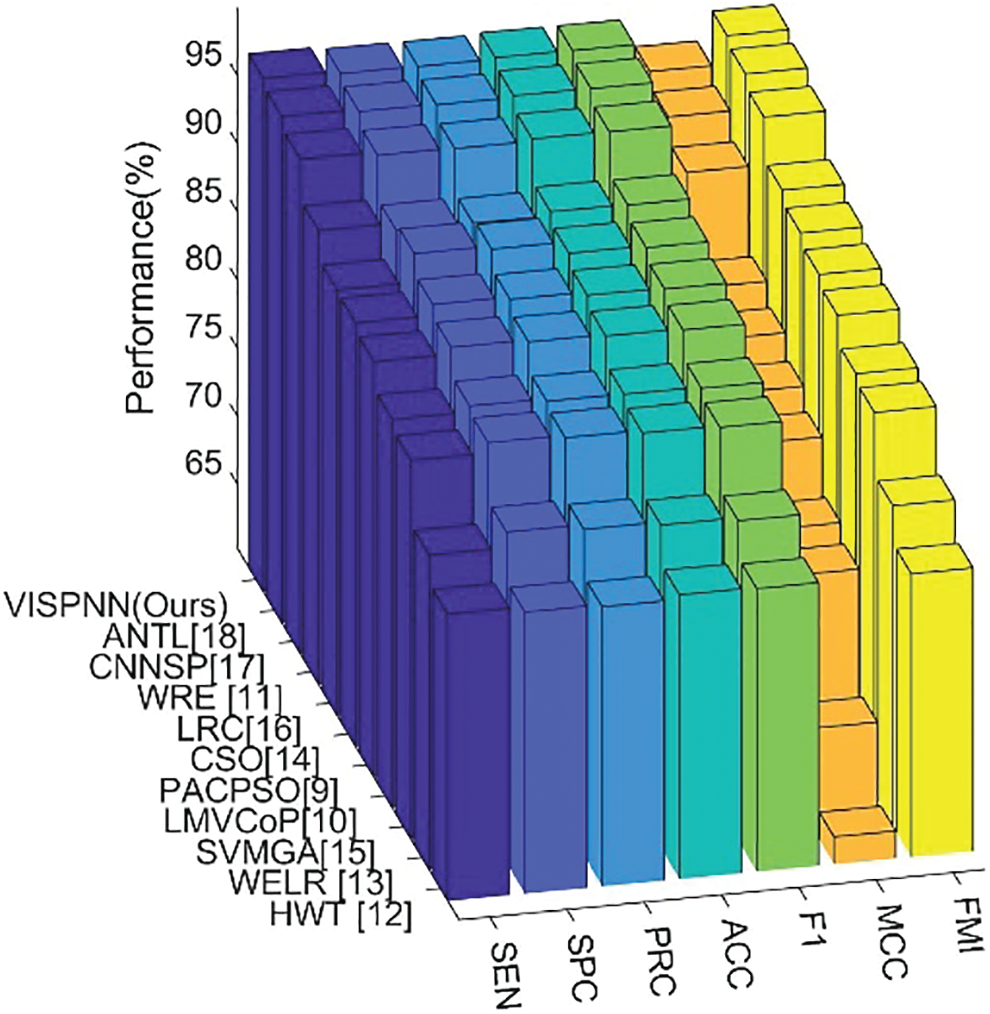
Figure 12: Bar plot of ranked 11 state-of-the-art methods in order of MCC

We can observe from Fig. 12 that the proposed VISPNN model beats all the other ten state-of-the-art methods in terms of all seven measures. The reason is three folds. First, the VGG-inspired mainstay network gains many benefits by mimicking the similar structures from VGG-16. Second, stochastic pooling helps our model more robust than max pooling does. Third, the improved 20-way data augmentation generates diverse fake training images to help our model more resistant to overfitting.

4  Conclusions

To identify alcoholism more efficiently, we propose the VISPNN model based on a VGG-inspired mainstay network, stochastic pooling technique, and an improved 20-way data augmentation. The results show that our model gains a sensitivity of 97.98 ± 1.32, a specificity of 97.80 ± 1.35, an accuracy of 97.89 ± 1.11, and an AUC of 0.9849, respectively. The performance is better than 10 state-of-the-art alcoholism recognition methods.

The limitations of this study are that this model does not go through strict clinician verification; also, the dataset is relatively small. Hence, we will try to collect more brain images of both alcoholism and healthy subjects. Meanwhile, we shall deploy our VISPNN model to the cloud server and invite clinicians and radiologists to use our web app and get their feedback to improve our model further.

Funding Statement: This paper is partially supported by the Royal Society International Exchanges Cost Share Award, UK (RP202G0230); Medical Research Council Confidence in Concept Award, UK (MC_PC_17171); Hope Foundation for Cancer Research, UK (RM60G0680); British Heart Foundation Accelerator Award, UK; Sino-UK Industrial Fund, UK (RP202G0289); Global Challenges Research Fund (GCRF), UK (P202PF11). In addition, we acknowledge the help of Dr. Hemil Patel and Dr. Qinghua Zhou for their help in English correction.

Conflicts of Interest: The authors declare that they have no conflicts of interest to report regarding the present study.

References

 1.  O. I. A. Hamid, L. M. E. Sabik, K. F. Abdelfadeel and S. F. Shaban, “Tramadol aggravates cardiovascular toxicity in a rat model of alcoholism: Involvement of intermediate microfilament proteins and immune-expressed osteopontin,” Journal of Biochemical and Molecular Toxicology, vol. 121, pp. 15, 2021. [Google Scholar]

 2.  D. A. Shirley, I. Sharma, C. A. Warren and S. Moonah, “Drug repurposing of the alcohol abuse medication disulfiram as an anti-parasitic agent,” Frontiers in Cellular and Infection Microbiology, vol. 11, pp. 7, 2021. [Google Scholar]

 3.  M. I. Airapetov, S. O. Eresko, A. A. Lebedev, E. R. Bychkov and P. D. Shabanov, “The role of toll-like receptors in neuroimmunology of alcoholism,” Biochemistry Moscow-Supplement Series B-Biomedical Chemistry, vol. 15, pp. 71–79, 2021. [Google Scholar]

 4.  J. L. Meyers, D. B. Chorlian, T. B. Bigdeli, E. C. Johnson, F. Aliev et al., “The association of polygenic risk for schizophrenia, bipolar disorder, and depression with neural connectivity in adolescents and young adults: Examining developmental and sex differences,” Translational Psychiatry, vol. 11, pp. 11, 2021. [Google Scholar]

 5.  N. T. Rachman, H. Tjandrasa and C. F. Ichah, “Alcoholism classification based on EEG data using independent component analysis (ICAwavelet de-noising and probabilistic neural network (PNN),” in Int. Seminar on Intelligent Technology and Its Applications, Lombok, Indonesia, pp. 17–20, 2016. [Google Scholar]

 6.  T. Bordia and N. M. Zahr, “The inferior colliculus in alcoholism and beyond,” Frontiers in Systems Neuroscience, vol. 14, pp. 19, 2020. [Google Scholar]

 7.  Q. Y. Zhao, M. Fritz, A. Pfefferbaum, E. V. Sullivan, K. M. Pohl et al., “Jacobian maps reveal under-reported brain regions sensitive to extreme binge ethanol intoxication in the rat,” Frontiers in Neuroanatomy, vol. 12, pp. 13, 2018. [Google Scholar]

 8.  C. E. Thompson, “The prodromal phase of alcoholism in Herman Melville’s Bartleby, the scrivener and cock-a-doodle-doo!,” Explicator, vol. 71, no. 4, pp. 275–280, 2013. [Google Scholar]

 9.  X.-X. Hou, “Alcoholism detection by medical robots based on Hu moment invariants and predator-prey adaptive-inertia chaotic particle swarm optimization,” Computers and Electrical Engineering, vol. 63, no. 6, pp. 126–138, 2017. [Google Scholar]

10. A. Jenitta and R. S. Ravindran, “Image retrieval based on local mesh vector co-occurrence pattern for medical diagnosis from MRI brain images,” Journal of Medical Systems, vol. 41, no. 10, Article ID: 157, 2017. [Google Scholar]

11. L. Han, “Identification of alcoholism based on wavelet Renyi entropy and three-segment encoded jaya algorithm,” Complexity, vol. 2018, Article ID: 3198184, 2018. [Google Scholar]

12. D. Lima, “Alcoholism detection in magnetic resonance imaging by Haar wavelet transform and back propagation neural network,” AIP Conference Proceedings, vol. 1955, Article ID: 040012, 2018. [Google Scholar]

13. F. Macdonald, “Alcoholism detection via wavelet energy and logistic regression,” Advances in Intelligent Systems Research, vol. 148, pp. 164–168, 2018. [Google Scholar]

14. P. Qian, “Cat swarm optimization applied to alcohol use disorder identification,” Multimedia Tools and Applications, vol. 77, no. 17, pp. 22875–22896, 2018. [Google Scholar]

15. Y. Chen, “Alcoholism detection by wavelet entropy and support vector machine trained by genetic algorithm,” in 27th IEEE Int. Conf. on Robot and Human Interactive Communication (ROMANNanjing, China, pp. 770–775, 2018. [Google Scholar]

16. X. Chen, “Alcoholism detection by wavelet energy entropy and linear regression classifier,” Computer Modeling in Engineering & Sciences, vol. 127, no. 1, pp. 325–343, 2021. [Google Scholar]

17. Y.-D. Lv, “Alcoholism detection by data augmentation and convolutional neural network with stochastic pooling,” Journal of Medical Systems, vol. 42, Article ID: 2, 2018. [Google Scholar]

18. S. Xie, “Alcoholism identification based on an alexnet transfer learning model,” Frontiers in Psychiatry, vol. 10, Article ID: 205, 2019. [Google Scholar]

19. C. Kamarajan, B. A. Ardekani, A. K. Pandey, D. B. Chorlian, S. Kinreich et al., “Random forest classification of alcohol use disorder using EEG source functional connectivity,” Behavioral Sciences, vol. 10, pp. 32, 2020. [Google Scholar]

20. A. Quaglieri, E. Mari, M. Boccia, L. Piccardi, C. Guariglia et al., “Brain network underlying executive functions in gambling and alcohol use disorders: An activation likelihood estimation meta-analysis of fmri studies,” Brain Sciences, vol. 10, pp. 19, 2020. [Google Scholar]

21. G. S. B. Jahangeer and T. D. Rajkumar, “Early detection of breast cancer using hybrid of series network and VGG-16,” Multimedia Tools and Applications, vol. 80, no. 5, pp. 7853–7886, 2021. [Google Scholar]

22. W. Y. Zhang, P. M. Shi, M. D. Li and D. Y. Han, “A novel stochastic resonance model based on bistable stochastic pooling network and its application,” Chaos Solitons & Fractals, vol. 145, pp. 10, 2021. [Google Scholar]

23. X. Cheng, “Psspnn: Patchshuffle stochastic pooling neural network for an explainable diagnosis of covid-19 with multiple-way data augmentation,” Computational and Mathematical Methods in Medicine, vol. 2021, Article ID: 6633755, 2021. [Google Scholar]

24. H. Akbari, M. T. Sadiq and A. U. Rehman, “Classification of normal and depressed EEG signals based on centered correntropy of rhythms in empirical wavelet transform domain,” Health Information Science and Systems, vol. 9, pp. 15, 2021. [Google Scholar]

This work is licensed under a Creative Commons Attribution 4.0 International License, which permits unrestricted use, distribution, and reproduction in any medium, provided the original work is properly cited.