Computers, Materials & Continua DOI:10.32604/cmc.2022.019711
Article

Magneto-Thermoelasticity with Thermal Shock Considering Two Temperatures and LS Model

F. S. Bayones1, S. M. Abo-Dahab2,3, N. S. Hussein4, A. M. Abd-Alla5,* and H. A. Alshehri1

1Department of Mathematics and Statistics, College of Science, Taif University, P.O. Box 11099, Taif, 21944, Saudi Arabia
2Mathematics Department, Faculty of Science, South Valley University, Qena, 83523, Egypt
3Computer Science Department, Faculty of Computers and Information, Luxor University, Luxor, Egypt
4Mathematics Department, Faculty of Science, Cairo University, Egypt
5Mathematics Department, Faculty of Science, Sohag University, Egypt
*Corresponding Author: A. M. Abd-Alla. Email: mohmrr@yahoo.com
Received: 23 April 2021; Accepted: 18 June 2021

Abstract: The present investigation is intended to demonstrate the magnetic field, relaxation time, hydrostatic initial stress, and two temperature on the thermal shock problem. The governing equations are formulated in the context of Lord-Shulman theory with the presence of bodily force, two temperatures, thermal shock, and hydrostatic initial stress. We obtained the exact solution using the normal mode technique with appropriate boundary conditions. The field quantities are calculated analytically and displayed graphically under thermal shock problem with effect of external parameters respect to space coordinates. The results obtained are agreeing with the previous results obtained by others when the new parameters vanish. The results indicate that the effect of magnetic field and initial stress on the conductor temperature, thermodynamic temperature, displacement and stress are quite pronounced. In order to illustrate and verify the analytical development, the numerical results of temperature, displacement and stress are carried out and computer simulated results are presented graphically. This study helpful in the development of piezoelectric devices.

Keywords: Thermoelastic; thermal shock; initial stress; two temperatures; magnetic field; relaxation time

1  Introduction

Recently, more attentions have been considered by researchers and engineers to the thermoelasticity theory to release the confliction of infinite speed due to the thermal signals, because of the importance in diverse fields as geophysics, acoustics, engineers, plasma physics, and industries. Biot [1] is the prior who presented the classical coupled thermoelasticity theory due to the coupled interaction between the thermal field and strain. The generalized thermoelasticity models have been introduced by Lord et al. [2] considering one relaxation time. Chen et al. [3] and Chen et al. [4,5] investigated the theory of heat conduction depending on two temperatures. Youssef [6] investigated the theory of two-temperature generalized thermoelasticity. Green et al. [7] who inserted two relaxation times and advocating finite wave speed thermal in solids by correcting the energy equation and Neuman-Duhamel relation or modifying Fourier’s conduction heat equation. Chandrasekharaiah et al. [8] studied the thermoelastic interactions without energy dissipation due to a point heat source. Chandrasekharaiah et al. [9] studied the temperature-rate-dependent thermo-elastic interactions due to a line heat source. The magnetoelastic earth’s material nature may affect on the wave propagation, especially surface waves. A literature review of the earliest contributions to the subject has been discussed in details by Puri [10]. Nayfeh et al. [11] who studied the plane wave propagation under the electromagnetic field in a solid medium. Choudhuri et al. [12] discussed the rotation effect on magneto-thermoelastic media in an elastic medium. Ezzat et al. [13] investigated the electromagneto-thermoelastic plane waves with two relaxation times in a medium of perfect conductivity Ezzat et al. [14] studied the electromagneto-thermoelastic plane waves with thermal relaxation in a medium of perfect conductivity. Zhuang et al. [15] studied the explicit phase field method for brittle dynamic fracture. Rabczuk et al. [16] investigated the nonlocal operator method for partial differential equations with application to the electromagnetic waveguide problem. Bahar et al. [17] introduced the formulation of state space in thermoelastic problems which also developed in Sherief [18] including the heat sources effectively. Sherief et al. [19] studied the two dimensional generalized thermoelasticity problem for an infinitely long cylinder. Youssef et al. [20] analysis a generalized thermoelastic infinite layer problem with the state space approach considering three models. Formulation of state space for the vibration of gold nano-beam in femtoseconds scale pointed out by Elsibai et al. [21]. Biot [22] clears that under stress free state would be fundamentally different from initial stresses states acoustic propagation and obtained the longitudinal and transverse wave velocities along the coordinate axes only. Chattopadhyay et al. [23] explained the plane wave reflection and refraction in an unbounded medium under initial stresses. Montanaro [24] studied the linear thermoelasticity problem with hydrostatic initial stress. Othman et al. [25] studied the reflection waves in a generalized thermoelastic medium from a free surface under hydrostatic initial stress under different thermoelastic theories. Youssef [26] studied the problem of generalized thermoelastic infinite medium with a cylindrical cavity subjected to a ramp-type heating and loads.

The main purpose of the present investigation is intended to demonstrate the magnetic field, relaxation time, hydrostatic initial stress, and two temperature on the thermal shock problem. The governing equations are formulated in the context of Lord-Shulman theory with the presence of body force, two temperatures, thermal shock, and hydrostatic initial stress. We obtained the exact solution using the normal mode technique with appropriate boundary conditions. The field quantities are calculated analytically and displayed graphically under thermal shock problem with effect of external parameters respect to space coordinates.

2  Formulation of the Problem

Considering that the medium is a perfect electric conductor and the absence of the displacement current (SI) [10], the linearized Maxwell equations governing the electromagnetic field as the form as shown in Fig. 1

curlh→=J→curlE→=−μe∂h→∂tdivh→=0,divE→=0where h→=curl(u→×H→0), H→=H→0+h→(x,y,t)(1)

in which h→ is the perturbed magnetic field over the primary magnetic field, J→ represents the electric current density, μe represents the magnetic permeability, H0 represents the constant primary magnetic field, and u→ represents the displacement vector, H→=(0,0,H0),u→=(u,v,0).

Figure 1: Schematic of the problem

The equation of heat conduction given [15] as

K(∂2φ∂x2+∂2φ∂y2)=(∂∂t+τ0∂2∂t2)ρCET+γT0(∂∂t+τ0∂2∂t2)(∂u∂x+∂v∂y)(2)

The stress–displacement relations for the isotropic material are

σxx=(2μ+λ)∂u∂x+λ∂v∂y−γT−P(3)

σyy=(2μ+λ)∂v∂y+λ∂u∂x−γT−P(4)

σxy=(μ+12P)∂u∂y+(μ−12P)∂v∂x,σyx=(μ+12P)∂v∂x+(μ−12P)∂u∂y(5)

The Maxwell’s equation formulated as

τij=μe[Hihj+Hjhi−Hk.hkδij](6)

The motion equation splits to

ρ∂2u∂t2=(λ+2μ+μeH02)∂2u∂x2+(λ+μ+12P+μeH02)∂2v∂x∂y+(μ−12P)∂2u∂y2−γT0∂T∂x(7)

ρ∂2v∂t2=(λ+2μ+μeH02)∂2v∂y2+(λ+μ+12P+μeH02)∂2u∂x∂y+(μ−12P)∂2v∂x2−γT0∂T∂y(8)

The heat conduction and dynamical heat related by the form

φ−T=a(∂2φ∂x2+∂2φ∂y2)(9)

The non-dimensional variables for simplifying gives as

σij′=σij2μ+λ,h′=h2μ+λ,P′=P2μ+λ,τ′=τ2μ+λ,(10)

where η=ρCEK, C22=μρ and c02=2μ+λρ

By dropping the dashed for convenience, and substitute Eq. (10), then Eqs. (2) and (9) take the following form

∇2φ−(1+τ0∂∂t)∂θ∂t−ε(1+τ0∂∂t)∂e∂t=0(11)

φ−θ=β(∂2φ∂x2+∂2φ∂y2)(12)

where ε=γρCE and β=aη2c02

Assuming the scalar and vector potential functions Π(x,y,t) and ψ(x,y,t) in the non-dimensional form defined as:

u=∂Π∂x+∂ψ∂y,v=∂Π∂y−∂ψ∂x(13)

By using (15) and (10) in Eqs. (7) and (8), we obtain.

[∇2−1a2∂2∂t2]Π−a∗θ=0(14)

(∇2−1a3∂2∂t2)ψ=0(15)

where a0=γT0ρC02, a1=ρC02μ, a2=1+Rh2, a∗=a0a2, a3=μ−12PρC02

Rh2 is the Alfven speed.

Also Eq. (11) tends to

∇2φ−(1+τ0∂∂t)∂θ∂t−ε(1+τ0∂∂t)∂∂t(∇2Π)=0(16)

3  The Solution to the Problem

The solution of the previous physical variables can be decomposed in terms of normal mode technique in the exponential harmonic form

[Π,ψ,φ,θ,σij](x,y,t)=[u∗(x),φ∗(x),θ∗(x),σij∗(x)]exp⁡(ωt+iby)(17)

where i=−1, b be a wave number, ω is the time constant, and u∗(x),φ∗(x),θ∗(x) and σij∗(x) are the amplitudes of the physical field quantities.

Using Eq. (17), into Eqs. (12) and (14)–(16), we obtain

[D2−A1]Π∗−A2θ∗=0(18)

[D2−b2]φ∗−Aθ∗+B[D2−b2]Π∗=0(19)

[D2−A3]φ∗=−β∗θ∗(20)

[D2−m2]ψ∗=0(21)

where A=ω(1+ωτ0),A1=b2+ω2a2,A2=a∗,A3=(βb2+1)/β,B=−εA, β∗=1β,m2=b2+ω2a3 and D=ddx

Solving Eqs. (18)–(20) by eliminating θ∗(x),Π∗(x), and φ∗(x), we obtain the partial differential equation satisfied by θ∗(x)

[D4−ED2+F]θ∗(x)=0(22)

where

E=A1+b2+βA(A1+A3)−βBA2(A3+b2)1+βA−βBA2,(23)

F=b2A1+βA3(AA1−BA2b2)1+βA−βBA2,(24)

Similarly, we get

[D4−ED2+F](Π∗,φ∗)(x)=0(25)

which can be factorized to

(D2−k12)(D2−k22)θ∗(x)=0(26)

where kn2(n=1,2) are the roots of the characteristic equation

k4−Ek2+F=0(27)

as x→∞, the solution of Eq. (26) is given by

θ∗(x)=∑n=12Mn(b,β,ω)exp⁡(−knx)(28)

Similarly

φ∗(x)=∑n=12Mn′(b,β,ω)exp⁡(−knx)(29)

Π∗(x)=∑n=12Mn′′(b,β,ω)exp⁡(−knx)(30)

The solution of Eq. (21) has the form

ψ∗(x)=M3e−mx.(31)

u∗(x)=DΠ∗+ibψ∗(32)

v∗(x)=ibΠ∗−Dψ∗(33)

e∗(x)=Du∗+ibv∗(34)

To get the amplitudes of the displacements u and v, which bounded as x→∞, then Eqs. (32) and (33) tend to

u∗(x)=−∑n=12Mn′′(b,β,ω)kne−knx+ibM3e−mx(35)

v∗(x)=∑n=12ibMn′′(b,β,ω)e−knx+mM3e−mx(36)

where Mn,Mn′ and Mn′′ are parameters depend on β,b and ω.

From Eqs. (28)–(30) into Eqs. (18)–(20), we get

Mn′(b,β,ω)=H1nMn(b,β,ω),n=1,2(37)

Mn′′(b,β,ω)=H2nMn(b,β,ω),n=1,2(38)

where

H1n=(β∗A3−kn2),n=1,2(39)

H2n=A2(kn2−A1),n=1,2(40)

Thus

φ∗(x)=∑n=12H1nMn(b,β,ω)exp⁡(−knx)(41)

Π∗(x)=∑n=12H2nMn(b,β,ω)exp⁡(−knx)(42)

Substitution of Eqs. (35) and (36) into Eqs. (3)–(5), we obtain

σxx∗=∑n=12hnMn(b,β,ω)exp⁡(−knx)−q1M3exp⁡(−mx)−P(43)

σyy∗=∑n=12hn′Mn(b,β,ω)exp⁡(−knx)+q1M3exp⁡(−mx)−P(44)

σxy∗=∑n=12hn′′Mn(b,β,ω)exp⁡(−knx)−q2M3exp⁡(−mx)(45)

τxx∗=∑n=12gnMn(b,β,ω)exp⁡(−knx),τyy∗=∑n=12gnMn(b,β,ω)exp⁡(−knx)(46)

where

hn=−(−H2nkn2+b2λH2n2μ+λ+γT02μ+λ)(47)

hn′=−(b2H2n−λH2nkn22μ+λ+γT02μ+λ)(48)

hn′′=−2ibμH2n2μ+λkn(49)

q1=ibm(1−λ2μ+λ)(50)

q2=μ(m2+b2)2μ+λ−12P(m2−b2)(51)

gn=−(−μeH022μ+λH2nkn2+μeH022μ+λb2H2n)(52)

The normal mode analysis is, in fact, to look for the solution in Fourier transformed domain. Assuming that all the field quantities are sufficiently smooth on the real line such that normal mode analysis of these functions exists.

4  Applications

Now we will obtain the parameters Mn(n=1,2,3), we will suppress the positive exponentials that are unbounded at infinity. The constants M1,M2,M3 must choose such that the boundary conditions on the surface atx=0 take the form:

Boundary conditions for the thermal at surface under thermal shock

θ(0,y,t)=f(0,y,t)(53)

Boundary condition for the mechanic at surface under initial stress

σxx(0,y,t)+τxx(0,y,t)=−P(54)

Boundary condition for the mechanic at the surface is traction free

σxy(0,y,t)+τxy(0,y,t)=0(55)

Substitute into the above boundary conditions in the physical quantities, we obtain

∑n=12Mn(b,β,ω)=f∗(y,t)(56)

∑n=12(hn+gn)Mn(b,β,ω)−q1M3=0(57)

∑n=12hn′′Mn(b,β,ω)−q2M3=0(58)

In the context of the boundary conditions in Eqs. (56)–(58) at the surface x=0, we get a system of three Algebraic equations, we will apply the inverse matrix method, we will get the three constants Mj, j=1,2,3, after that by substituting into the main expressions to obtain the displacements, temperature and other physical quantity.

5  Numerical Results and Discussions

To illustrate the analytical variable obtained earlier, we will consider a numerical example consider copper material. The results display the variation of displacements, temperature and stress in the context of LS theory.

We took the constants: y=−1, time t=0.1, b=0.25,H=105,P=1010,β=0.1,τ=0.1 for all computations, and we used for the real part of the displacement u,v, strain e and the stresses (σxx,σyy,σxy), thermal temperature θ and conductive temperature ϕ. All the field quantities don’t depend only on space x and time t, also on the relaxation time τ and in dimensionless form:

The output is plotted in Figs. 2–7.

Figure 2: Conductive temperature ϕ with respect to x and variation of t, b, β, τ, H and P

Figure 3: Thermodynamical temperature θ with respect to x and variation of t, b, β, τ, H and P

Figure 4: Displacement u with respect to x and variation of t, b, β, τ, H and P

Figure 5: Displacement v with respect to x and variation of t, b, β, τ, H and P

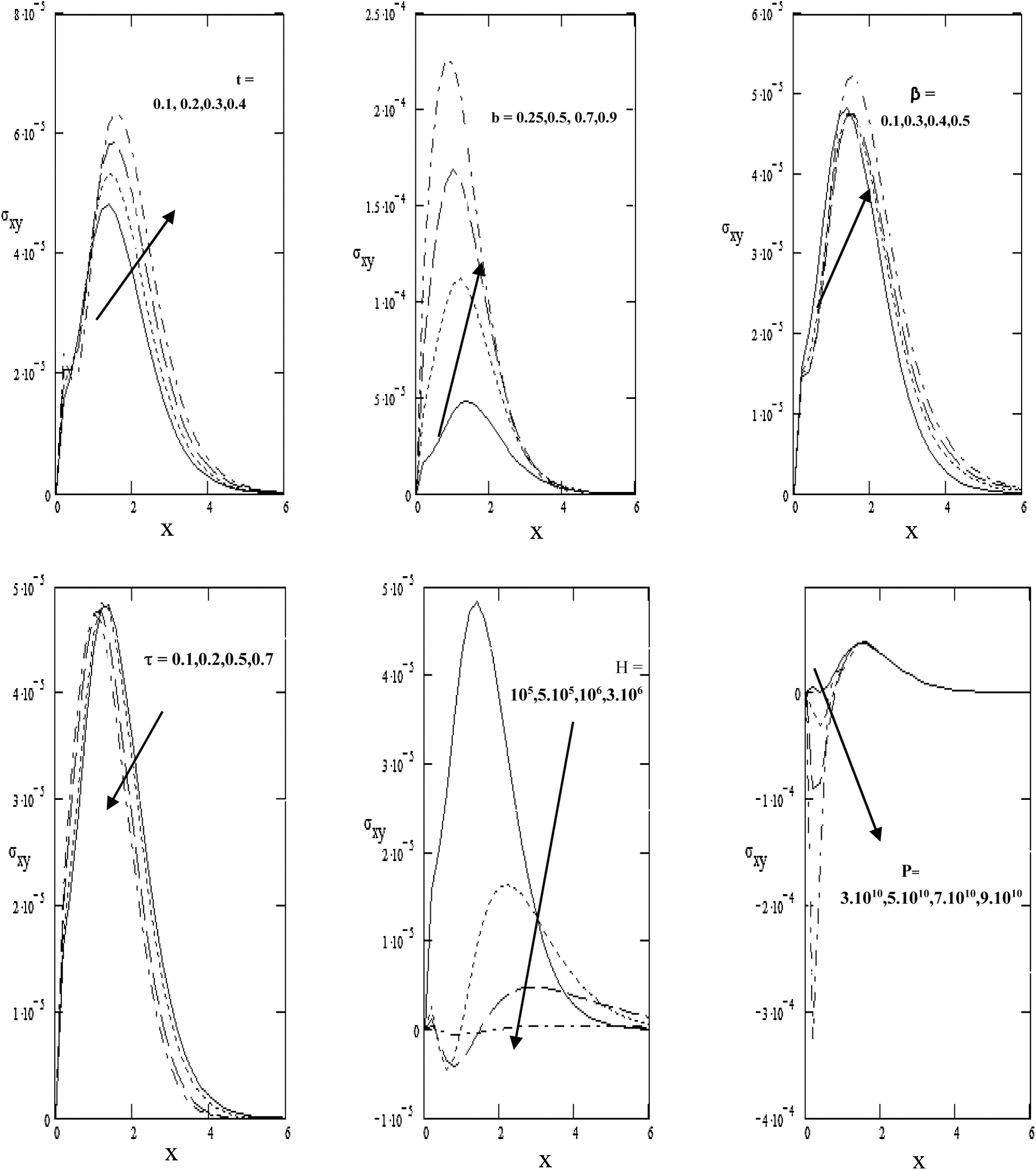
Figure 6: Stress σxy with respect to x and variation of t, b, β, τ, H and P

Figure 7: Stress σyy with respect to x and variation of t, b, β, τ, H and P

Fig. 2 displays the values of the conductive temperature ϕ, which decreases with increasing of axial x. They indicate that the medium along the axial x tends to zero as x tends to infinity. The effect of time t, wave number b, longitudinal wave velocity, β, relaxation time τ, magnetic field H and initial stress P on the conductive temperature. The conductive temperature increases with increasing of time and longitudinal wave velocity, while it decreases with increasing of wave number and relaxation time, also, there isn’t any effect due to the magnetic field and initial stress on the conductive temperature.

Fig. 3 plots the values of the thermodynamic temperature θ, which decreases with increasing of axial x. These figures indicate that the medium along axial x. The effect of time t, wave number b, longitudinal wave velocity β, relaxation time τ, magnetic field H and initial stress P on the conductive temperature. The thermodynamic temperature increases with increasing of time and longitudinal wave velocity, while it decreases with increasing of wave number and relaxation time, as well, there is no effect of magnetic field and initial stress on the thermodynamic temperature.

Fig. 4 shows the values of displacement u, which has an oscillatory behavior in the whole range of axial x under the effects of time t, wave number b, longitudinal wave velocity β, relaxation time τ, magnetic field H and initial stress P. In these figures, it is clear that the displacement has a nonzero value only in the bounded region of space, while it increases with increasing of time, wave number and longitudinal wave velocity, as well it decreases with increasing relaxation time and magnetic field, while there is no effect of initial stress on the displacement.

Fig. 5 displays the value of displacement v which has an oscillatory behavior in the whole range of axial x under the effects of time t, wave number b, longitudinal wave velocity, β, relaxation time τ, magnetic field H and initial stress P. In these figures, it is clear that the displacement has a non-zero value only in the bounded region of space, while it increases with increasing of time, wave number and longitudinal wave velocity, as well it decreases with increasing relaxation time and magnetic field, while there is no effect of initial stress on the displacement.

Fig. 6 clears the values of stress, σxy which has an oscillatory behavior in the whole range of axial x under the effects of time t, wave number b, longitudinal wave velocity, β, relaxation time τ, magnetic field H and initial stress P. In these figures, it is clear that the stress has a nonzero value only in the bounded region of space, while it increases with increasing of time, wave number and longitudinal wave velocity, as well it decreases with increasing temperature, magnetic field and initial stress.

Fig. 7 shows the values of the stress σyy, which increases with increasing of axial x. These figures indicate that the medium along axial x the effect of time t, wave number b, longitudinal wave velocity, β, relaxation time τ, magnetic field H and initial stress P on the stress. The stress decreases with increasing of time, wave number, longitudinal wave velocity and initial stress, while it increases with increasing relaxation time, as well, there is no effect of magnetic field on the stress.

6  Conclusion

The results and conclusions can be summarized as follows

Normal mode analysis of the problem of magneto-thermoelastic solid has been applied and developed.

The generalized magneto-thermoelasticity with thermal shock, two temperatures, initial stress described with characteristic by fourth order equation.

The role of the initial stress, thermal shock, magnetic field clears strongly on the physical quantities depending on the nature of the medium, horizontal and vertical distances x and y respectively. The nature of forced applied as well as the type of boundary conditions deformation.

Finally, it is concluded that all the external parameters affect strongly on the physical quantities of the phenomenon which has more applications, especially, in engineering, geophysics, astronomy, acoustics, industry, structure, and other related topics.

Acknowledgement: Taif University Researchers Supporting Project Number (TURSP-2020/164), Taif University, Taif, Saudi Arabia.

Funding Statement: The authors received no specific funding for this study.

Conflicts of Interest: The authors declare that they have no conflicts of interest to report regarding the present study.

References

 1.  M. A. Biot, “Thermoelasticity and irreversible thermodynamics,” Journal of Applied Physics, vol. 27, no. 1, pp. 240–253, 1956. [Google Scholar]

 2.  H. W. Lord and Y. Shulman, “A generalized dynamical theory of thermo-elasticity,” Journal of the Mechanics and Physics of Solids, vol. 15, no. 5, pp. 299–309, 1967. [Google Scholar]

 3.  P. J. Chen and M. E. Gurtin, “On a theory of heat conduction involving two temperatures,” Zeitschrift für Angewandte Mathematik und Physik, vol. 19, no. 1, pp. 614–627, 1968. [Google Scholar]

 4.  P. J. Chen, M. E. Gurtin and W. O. Williams, “A note on non-simple heat conduction,” Zeitschrift für Angewandte Mathematik und Physik, vol. 19, no. 1, pp. 969–970, 1968. [Google Scholar]

 5.  P. J. Chen, M. E. Gurtin and W. O. Williams, “On the thermodynamics of non-simple elastic materials with two temperatures,” Zeitschrift für Angewandte Mathematik und Physik, vol. 20, no. 1, pp. 107–112, 1969. [Google Scholar]

 6.  H. M. Youssef, “Theory of two-temperature generalized thermoelasticity,” IMA Journal of Applied Mathematics, vol. 71, no. 1, pp. 383–390, 2006. [Google Scholar]

 7.  E. Green and K. A. Lindsay, “Thermoelasticity,” Journal of Elasticity, vol. 2, no. 1, pp. 1–7, 1972. [Google Scholar]

 8.  D. S. Chandrasekharaiah and K. S. Srinath, “Thermoelastic interactions without energy dissipation due to a point heat source,” Journal of Elasticity, vol. 50, no. 2, pp. 97–108, 1998. [Google Scholar]

 9.  D. S. Chandrasekharaiah and H. N. Murthy, “Temperature-rate-dependent thermo-elastic interactions due to a line heat source,” Acta Mechanica, vol. 89, no. 3, pp. 1–12, 1991. [Google Scholar]

10. P. Puri, “Plane waves in thermoelasticity and magneto-thermoelasticity,” International Journal of Engineering Science, vol. 10, no. 5, pp. 467–476, 1972. [Google Scholar]

11. A. Nayfeh and S. Nemat-Nasser, “Transient thermoelastic waves in half-space with thermal relaxation,” Zeitschrift für Angewandte Mathematik und Physik, vol. 23, no. 1, pp. 52–68, 1972. [Google Scholar]

12. S. K. R. Choudhuri and S. Mukhopdhyay, “Effect of rotation and relaxation on plane waves in generalized thermo-viscoelasticity,” International Journal of Science and Mathematics Science, vol. 23, no. 7, pp. 479–505, 2000. [Google Scholar]

13. M. A. Ezzat and M. I. A. Othman, “Electromagneto-thermoelastic plane waves with two relaxation times in a medium of perfect conductivity,” International Journal of Engineering Science, vol. 38, no. 1, pp. 107–120, 2000. [Google Scholar]

14. M. Ezzat, M. I. A. Othman and A. S. El-Karamany, “Electromagneto-thermoelastic plane waves with thermal relaxation in a medium of perfect conductivity,” Journal of Thermal Stresses, vol. 24, no. 5, pp. 411–432, 2001. [Google Scholar]

15. H. L. Ren, X. Y. Zhuang, C. Anitescu and T. Rabczuk, “An explicit phase field method for brittle dynamic fracture,” Computers and Structures, vol. 217, no. 1, pp. 45–56, 2019. [Google Scholar]

16. T. Rabczuk, H. Ren and X. Zhuang, “A nonlocal operator method for partial differential equations with application to electromagnetic waveguide problem,” Computers, Materials and Continua, vol. 59, no. 1, pp. 31–55, 2019. [Google Scholar]

17. L. Y. Bahar and R. Hetnarski, “State space approach to thermoelasticity,” Journal of Thermal Stresses, vol. 1, no. 1, pp. 135–145, 1978. [Google Scholar]

18. H. Sherief, “State space formulation for generalized thermoelasticity with one relaxation time including heat sources,” Journal of Therm. Stresses, vol. 16, no. 2, pp. 163–176, 1993. [Google Scholar]

19. H. Sherief and M. Anwar, “A two dimensional generalized thermoelasticity problem for an infinitely long cylinder,” Journal of Therm. Stresses, vol. 17, no. 2, pp. 213–227, 1994. [Google Scholar]

20. H. M. Youssef and A. A. El-Bary, “Mathematical model for thermal shock problem of a generalized thermoelastic layered composite material with variable thermal conductivity,” Mathematical Problems in Engineering, vol. 12, no. 2, pp. 165–171, 2006. [Google Scholar]

21. K. Elsibai and H. Youssef, “State space formulation to the vibration of gold nano-beam induced by ramp type heating without energy dissipation in femtoseconds scale,” Journal of Therm. Stresses, vol. 34, no. 3, pp. 244–263, 2011. [Google Scholar]

22. M. A. Biot, Mechanics of Incremental Deformations, New York, NY, USA: John Wiley & Sons, 1965. [Google Scholar]

23. S. Chattopadhyay, S. Bose, and M. Chakraborty, “Reflection of elastic waves under initial stress at a free surface: P and SV motion,” Journal of the Acoustical Society of America, vol. 72, no. 1, pp. 255–263, 1982. [Google Scholar]

24. A. Montanaro, “On singular surfaces in isotropic linear thermoelasticity with initial stress,” Journal of the Acoustical Society of America, vol. 106, no. 3, pp. 1586–1588, 1999. [Google Scholar]

25. M. I. A. Othman and Y. Song, “Reflection of plane waves from an elastic solid half-space under hydrostatic initial stress without energy dissipation,” International Journal of Solids and Structures, vol. 44, no. 17, pp. 5651–5664, 2007. [Google Scholar]

26. H. Youssef, “Problem of generalized thermoelastic infinite medium with cylindrical cavity subjected to a ramp-type heating and loading,” Archive of Applied Mechanics, vol. 75, no. 4, pp. 553–565, 2006. [Google Scholar]

This work is licensed under a Creative Commons Attribution 4.0 International License, which permits unrestricted use, distribution, and reproduction in any medium, provided the original work is properly cited.