Computers, Materials & Continua DOI:10.32604/cmc.2022.020140
Article

Deep Rank-Based Average Pooling Network for Covid-19 Recognition

Shui-Hua Wang1, Muhammad Attique Khan2, Vishnuvarthanan Govindaraj3, Steven L. Fernandes4, Ziquan Zhu5 and Yu-Dong Zhang6,*

1School of Mathematics and Actuarial Science, University of Leicester, LE1 7RH, UK
2Department of Computer Science, HITEC University Taxila, Taxila, Pakistan
3Department of Biomedical Engineering, Kalasalingam Academy of Research and Education, 626 126, Tamil Nadu, India
4Department of Computer Science, Design & Journalism, Creighton University, Omaha, Nebraska, USA
5Science in Civil Engineering, University of Florida, Gainesville, Florida, FL 32608, USA
6School of Informatics, University of Leicester, UK
*Corresponding Author: Yu-Dong Zhang. Email: yudongzhang@ieee.org
Received: 11 May 2021; Accepted: 18 June 2021

Abstract: (Aim) To make a more accurate and precise COVID-19 diagnosis system, this study proposed a novel deep rank-based average pooling network (DRAPNet) model, i.e., deep rank-based average pooling network, for COVID-19 recognition. (Methods) 521 subjects yield 1164 slice images via the slice level selection method. All the 1164 slice images comprise four categories: COVID-19 positive; community-acquired pneumonia; second pulmonary tuberculosis; and healthy control. Our method firstly introduced an improved multiple-way data augmentation. Secondly, an n-conv rank-based average pooling module (NRAPM) was proposed in which rank-based pooling—particularly, rank-based average pooling (RAP)—was employed to avoid overfitting. Third, a novel DRAPNet was proposed based on NRAPM and inspired by the VGG network. Grad-CAM was used to generate heatmaps and gave our AI model an explainable analysis. (Results) Our DRAPNet achieved a micro-averaged F1 score of 95.49% by 10 runs over the test set. The sensitivities of the four classes were 95.44%, 96.07%, 94.41%, and 96.07%, respectively. The precisions of four classes were 96.45%, 95.22%, 95.05%, and 95.28%, respectively. The F1 scores of the four classes were 95.94%, 95.64%, 94.73%, and 95.67%, respectively. Besides, the confusion matrix was given. (Conclusions) The DRAPNet is effective in diagnosing COVID-19 and other chest infectious diseases. The RAP gives better results than four other methods: strided convolution, l2-norm pooling, average pooling, and max pooling.

Keywords: COVID-19; rank-based average pooling; deep learning; deep neural network

1  Introduction

COVID-19 has caused over 158.3 million confirmed cases, with over 3.29 million death tolls till 9/May/2021. The key symptoms of COVID-19 are high temperature, new and continuous cough, and loss or change to smell or taste [1]. Most people have mild symptoms, but some people may develop acute respiratory distress syndrome, which may trigger multi-organ failure, blood clots, septic shock, and cytokine storm.

The real-time reverse-transcriptase polymerase chain reaction technique is the main viral testing method. It usually picks the nasopharyngeal swab trials to test the presence of RNA pieces of the virus. Nevertheless, the swab could be easily contaminated, and it takes hours to two days to wait for the results [2]. Hence, chest imaging is used as an alternative way to diagnose COVID-19. Chest computed tomography (CCT) is the dominant chest imaging method compared to chest radiography and chest ultrasound since CCT can provide 3D chest imaging scans with the finest resolutions. Particularly, Ai et al. [3] carried out a large study comparing CCT against rRT-PCR, and found CCT is faster and more sensitive.

The lesions of COVID-19 in CCT are shown with main symptoms of regions of ground-glass opacity (GGO). The manual recognition works by radiologists are labor-intensive, and tedious. The manual labelling is probable to be influenced by many factors (emotion, fatigue, lethargy, etc.). In contrast, machine learning (ML) always strictly follows the instruction designed more quickly and more reliably than humans. Furthermore, the lesions of early-phase of COVID-19 patients are small and trivial, like to the nearby healthy tissues, that can be easily detected by ML algorithms meanwhile probably ignored by human radiologists.

There have been many ML methods proposed this year to recognize COVID-19 or other related diseases. Roughly speaking, those methods can be divided into traditional ML methods [4,5] and deep learning (DL) methods [6–10]. However, the performance of all those methods can still be improved. Hence, this study presents a novel DL approach: rank-based average pooling neural network with PatchShuffle (RAPNNSP). The contributions of this study entail the following four points:

(i)   An improved 18-way data augmentation technique is introduced to aid the model from overfitting.

(ii)   An “n-conv rank-based average pooling module (NRAPM)” is presented.

(iii)   A new “Deep RAP Network (DRAPNet)” is proposed inspired by VGG-16 and NRAPM.

(iv)   Grad-CAM is utilized to prove the explainable heat map that links with COVID-19 lesions.

2  Background on COVID-19 Detection Methods

In this Section, we briefly discuss the recent ML methods for detecting COVID-19 and other diseases. Those methods will be used as a comparison baseline in our experiment. Wu [4] used wavelet Renyi Entropy (WRE) as the feature extraction; and presented a new “three-Segment Biogeography-Based Optimization” as the classifier. Li et al. [5] used wavelet packet Tsallis entropy as a feature descriptor. The authors based on biogeography-based optimization (BO), presented a real-coded BO (RCBO) as the classifier.

The pipeline of traditional ML methods [4,5] could be categorized into two stages: feature extraction and classification. Those methods show good results in detecting COVID-19. Traditional ML methods suffer from two points: (i) a long time of feature engineering; and (ii) low performance. To solve the above two issues, modern deep neural networks, e.g., convolutional neural networks (CNNs), have been investigated and applied to COVID-19.

For instance, Cohen et al. [6] presented a COVID severity score network (CSSNet). The experiments show that the mean absolute error (MAE) is 0.78 on lung opacity score, and MAE is 1.14 on geographic extent score. Afterward, Li et al. [7] presented a fully automatic model to recognize COVID-19 via CCT. This model is dubbed COVNet. Zhang [8] presented a 7-layer convolutional neural network for COVID-19 diagnosis (CCD). The performance yielded an accuracy of 94.03 ± 0.80 for COVID-19 against healthy people. Ko et al. [9] presented a fast-track COVID-19 classification framework (FCONet in short). Wang et al. [10] proposed DeCovNet, which is a 3D deep CNN to detect COVID-19. When using a probability threshold of 0.5, DeCovNet attained a 0.901 accuracy. Erok et al. [11] presented the imaging features of the early phase of COVID-19.

The above DL methods yield promising results in recognizing COVID-19. In order to get better results, we study the structures of those neural networks, and present a novel DRAPNet approach, by using the mechanisms of four cutting-edge approaches: (i) multiple-way data augmentation, (ii) VGG network, (iii) rank-based average pooling, and (iv) Grad-CAM.

3  Dataset and Preprocessing

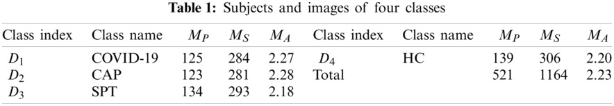
Our retrospective study was exempted by the Institutional Review Boards of local hospitals. The details of the dataset were described in Ref. [12]. 521 subjects yielded 1164 slice images via the slice level selection (SLS) method. Four types of CCT were included in the dataset: (a) COVID-19 positive; (b) community-acquired pneumonia (CAP); (c) second pulmonary tuberculosis (SPT); (d) healthy control (HC).

SLS chooses m={1,2,3,4} slices for each subject. The average number of selected slices (ANSS, denoted by a variable MA) per class is defined as MA(Dk)=MS(Dk)MP(Dk),k=1,⋯,4, where Dk is the category, MS and MP stand for the number of slices by SLS, and the number of patients, respectively. The entire ANSS is defined as MA=∑k=14⁡MS(Dk)/∑k=14⁡MP(Dk). Tab. 1 shows the demographics of the four-class subject cohort; and their corresponding triplets [MP,MS,MA], where MA of the entire set is 2.23.

Three skilled radiologists (2 juniors: A1 and A2, 1 senior: B1) are called together to curate all the images. Suppose a means one CCT slice image, g stands for the labelling. The last labelling gF of the CCT scan a is defined as:

gF[a]={g[A1,a]g[A1,a]==g[A2,a]fMV{gall[a]}otherwise,(1)

where fMV stands for majority voting, gall the labelling concatenation of all 3 radiologists (A1,A2,B1), viz., gall[a]=[g(A1,a),g(A2,a),g(B1,a)].

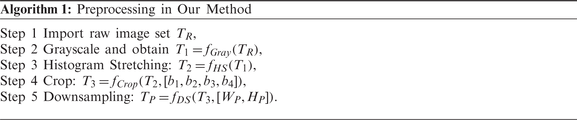
Define the dataset is T with five stages: the raw dataset TR, the final preprocessed output TP, and three temporary output T1,T2,T3. The flowchart of preprocessing is displayed in Fig. 1. Let |T| denotes the number of images in the dataset, which keeps the same for all five stages.

Figure 1: Illustration of preprocessing

The original raw dataset contained |T| slice images TR={tr(i),i=1,2,⋯,|T|}. The size of each image is size[tr(i)]=1024×1024×3. The colorful CCT images from four classes (D1,D2,D3,D4) are transformed into grayscale versions by reserving the luminance channel. We yield the grayscale image set T1=fGray(TR), in which fGray stands for the grayscale operation. Note TR are stored in three color channels, so the gray-scaling is necessary to reduce the storage.

Second, the histogram stretching (HS) is introduced for contrast-enhancement of all |T| images. Select the i-th image t1(i),i=1,2,⋯,|T| as an example, the minimum and maximum grayscale values t1l(i) and t1h(i) are reckoned as:

{t1l(i)=minw=1W1minh=1H1t1(i∣w,h),t1h(i)=maxw=1W1maxh=1H1t1(i∣w,h),(2)

where (w, h) mean the indexes of width and height directions of the image t1(i), respectively. (W1,H1) stand for the width and height of the image set T1. The recent histogram stretched data set T2 is evaluated image-dependently, i.e., we calculate the minimum and maximum grayscale values for each image.

T2=fHS(T1)={t2(i)=deft1(i)−t1l(i)t1h(i)−t1l(i)},(3)

where fHS means the histogram stretching operation.

Third, cropping is carried out to get rid of the checkup bed at the bottom area (See Fig. 1), and to remove the scripts at the corner regions. The cropped dataset T3 is defined as: T3=fCrop(T2,[b1,b2,b3,b4]), where fCrop represents crop operation. Parameters (b1,b2,b3,b4) means lengths to be cropped along four ways (top, bottom, left, and right), measured by pixels. Here the parameters (b1,b2,b3,b4) are image-independent, so they apply for all images in the dataset T2.

Fourth, each image in T3 is downsampled to a new image with the size of [WP,HP], yielding the final downsized data set TP=fDS(T3,[WP,HP]), where fDS:x↦y stands for the downsampling process, where y represents the down-sampled image of the original image x. The summary of the preprocessing of our method is listed in Algorithm 1.

4  Methodology

4.1 Enhanced Training Set by 18-way Data Augmentation

The preprocessed dataset TP is split into two parts: non-test set (80%) and test set (20%). Ten-fold cross-validation is performed on the non-test set to choose the optimal hyperparameter (including network structure). Afterward, 10 runs on the test set are carried out to report the test performance.

Data augmentation (DA) is an important tool to avoid overfitting and overcome the small-size dataset problem. DA has been proven to show excellent performances in many prediction/recognition/classification tasks, such as stock market prediction, prostate segmentation, etc. Recently, Wang [13] proposed a novel multiple-way data augmentation (MDA). In their 14-way DA [13], the inventors utilized seven different DA methods to the original slice tp(i) and its horizontal mirrored one tpM(i), respectively. Later, Zhu [14] presented an 18-way DA, where they added salt-and-pepper noise (SAPN) and speckle noise (SN) to the original 14-way DA. We use the latter one, 18-way DA, in this study.

Suppose NW stands for the number of ways of DA, that is, NW=18 in this study. For a given preprocessed image tp(x,y),x=1,⋯,WP,y=1,⋯,HP, the SAPN altered image is defined as tpSAPN(x,y), we get

Pr(tpSAPN=tp)=1−aDSAPN,Pr(tpSAPN=vmin)=aDSAPN2,Pr(tpSAPN=vmax)=aDSAPN2(4)

where aDSAPN stands for noise density, and Pr is the probability function. vmin and vmax stand for the minimum value and maximum value of the graylevel image can have, which correspond to black and white colors, respectively. The SN altered image is defined as tPSN(x,y)=tP(x,y)+N∗tp(x,y), where N is uniformly distributed random noise. The mean and variance of N are set to 0 and 0.05, respectively.

Let NI represent the number of newly generated images for each DA, we can present the 18-way DA algorithm as follows: First, nine geometric/photometric/noise-injection DA transforms are utilized on raw image tp(i),i=1,⋯,|T|. We use f(m)DA,m=1,…,NW2 to stand for each DA operation. It is noteworthy each DA operations fkDA generates NI fake images. Therefore, a given image tp(i) can generate nine different data set f(m)DA[tp(i)],m=1,⋯,NW2.

Second, a horizontally mirrored image is generated as tpM(i)=fM[tp(i)], where fM means horizontal mirror function.

Third, all the nine DA methods are carried out on the horizontally mirrored image tpM(i), which generates nine new datasets f(m)DA[tpM(i)],m=1,⋯,NW2.

Fourth, the original image tP(i), the horizontally mirrored image tpM(i), all the 9-way DA results of the original image f(m)DA[tp(i)],m=1,⋯,NW2, and 9-way DA results of horizontal mirrored image f(m)DA[tpM(i)],m=1,⋯,NW2, are combined using concatenation function fCON. The final combined dataset is defined as T(i)

tp(i)↦T(i)=fcon{tp(i)f(1)DA[tp(i)]⏟NI⋯f(NW/2)DA[tp(i)]⏟NItpM(i)f(1)DA[tpM(i)]⏟NI⋯f(NW/2)DA[tpM(i)]⏟NI}(5)

Therefore, one image tp(i) will generate |T(i)|=NW∗NI+2 images (including original image). Algorithm 2 itemizes the pseudocode of 18-way DA on one image.

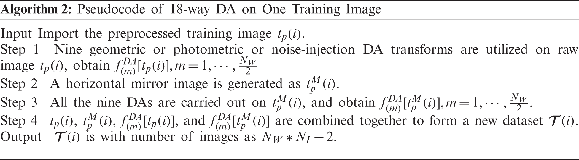
Fig. 2 shows the Step 2 result of this proposed 18-way DA results, i.e., f(m)DA[tp(i)],m=1,…,NW2. Due to the page limit, other components, viz., tpM(i) and f(m)DA[tpM(i)],m=1,⋯,NW2 are now displayed here. The raw image is Fig. 7a.

Figure 2: Results of 18-way data augmentation (a) Gaussian noise (b) SAPN (c) SN (d) Horizontal shear (e) Vertical shear (f) Image rotation (g) Scaling (h) Random translation (i) Gamma correction

4.2 Proposed n-Conv Rank-Based Pooling Module

In the standard CNNs, pooling is an essential module after each convolution layer to shrink the spatial sizes of feature maps (SSFMs). Recently, strided convolution (SC) is commonly used, which also reduces SSFMs. Nevertheless, SC might be thought of as a simple pooling method, which always outputs the fixed-position value in the pooling region. In this work, we use rank-based average pooling (RAP) [15] to replace traditional max pooling. Further, RAP has been reported to yield better operation than max pooling and average pooling in up-to-date studies.

Suppose there is a post-convolution feature map (FM) assigned with a variable of H=hij(i=1,⋯,M×R,j=1,⋯,N×R). The FM could dissent into M×N blocks, where the size of each block is R×R. Let us aim at the block Dmn that means the m-th row and n-th column block. The elements in the block Dmn is defined as Dmn={d(x,y),x=1,⋯,R,y=1,⋯,R}.

The strided convolution (SC) traverses the input FM with strides that equal to the block’s size (R,R); thus, its output is always the first element in the pooling region Dmn. The l2-norm pooling (L2P), max pooling (MP), and average pooling (AP) engender the l2-norm value, maximum value, and average value of the block Dmn, respectively. Let O be the pooling output, we have:

{OSC(Dmn)=d(1,1),OL2P(Dmn)=∑x=1R⁡∑y=1R⁡d2(x,y)R2,OMP(Dmn)=maxx=1Rmaxy=1Rd(x,y),OAP(Dmn)=1R×R∑x=1R⁡∑y=1R⁡d(x,y).(6)

Note that the ordinary convolutional neural network (CNN) can be combined with all the above four techniques, and we can attain SC-CNN, L2P-CNN, MP-CNN, and AP-CNN, respectively. Those four methods will be utilized as comparison baselines in the experiment.

The RAP is not a value-based pooling; in contrast, SP is a type of rank-based pooling. The output of RAP is based on ranks of pixels other than values of pixels in the block Dmn. Thus, RAP could solve the shortcomings of MP and AP. MP outputs the maximum value but worsens the overfitting challenge. Oppositely, the AP produces the average, with the shortcoming of downscaling the largest value, where the important traits may be contained.

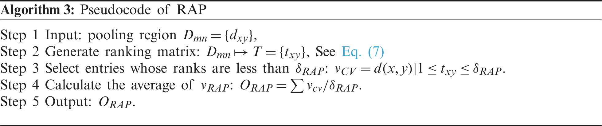
RAP is a three-step route. First, the ranking matrix (RM) T={txy} is generated from the pooling region, where x=1,⋯,R, y=1,⋯,R and txy∈[1,2,⋯,R×R]. In all, T is generated by the rule: the less value the entry is, the higher value the rank is. If tied values are for d(x1,y1) and d(x2,y2), then we check the index values of x1 and x2. If x1 equals x2, then we check the value of y1 and y2.

{d(x1,y1)<d(x2,y2)→t(x1,y1)>t(x2,y2),[d(x1,y1)==d(x2,y2)]∧(x1>x2)→t(x1,y1)>t(x2,y2),[d(x1,y1)==d(x2,y2)]∧(x1==x2)∧(y1>y2)→t(x1,y1)>t(x2,y2).(7)

Second, select the pixels whose ranks are no more than a threshold δRAP, which controls how many pixels within a region will be considered. The selected elements are rearranged into a candidate vector (CV) as vCV={d(x,y)|1≤txy≤δRAP}.

Third, the average CV vRAP is output as final RAP output:

ORAP(Dmn)=1δRAP∑⁡vCV=1δRAP∑⁡d(x,y)|1≤txy≤δRAP.(8)

Algorithm 3 shows the pseudocode of RAP. Fig. 3 shows the comparison of four different pooling methods, where δRAP=4 and R=3. Select the top-left block (in red rectangle) as an example, it contains 9 entries as: 2.4, 8.9, 4.9, 9.2, 9.5, 0.5, 3.4, 5.4, and 3.4. The L2P, AP, and MP output 6.88, 6.29, and 9.5 respectively, using Eq. (6). In contrast, RAP first calculate the RM and selects the δRAP greatest entries, i.e., vRAP=(9.5,9.5,9.2,8.9). The average of vRAP is the output of RAP, thus ORAP=9.28.

Figure 3: Comparison of four pooling methods

The second contribution of this study is that we proposed a new “n-conv rank-based average pooling module” (NRAPM) based on RAP layer. The NRAPM is composed of n-repetitions of a conv layer and a BN layer, followed by a RAP layer. Fig. 4 displays the graph of the proposed NRAPM. We set 1≤n≤3, because we run our model using n>3 on training set, but the validation performance of n>3 did not improve. ReLU function is missing in Fig. 4.

Figure 4: Schematic of proposed NRAPM

4.3 DRAPNet: Deep RAP Network

The final contribution of this study is to propose a deep RAP network (DRAPNet) with its conv block being NRAPM and its structure inspired by VGG-16 [16]. Fig. 5 displays the structure of VGG-16, which entails five conv layers and three dense layers (i.e., fully connected layer). The input of VGG-16 is 224×224×3. After the 1st convolution block (CB), that entails (i) two repetitions of 2 convolutional layers with 64 kernels whose sizes are 3×3, and (ii) one max pooling layer with a size of 2×2. The 1st CB is abbreviated as “2 × (64 3 × 3)”. The output of 1st CB is 112×112×64.

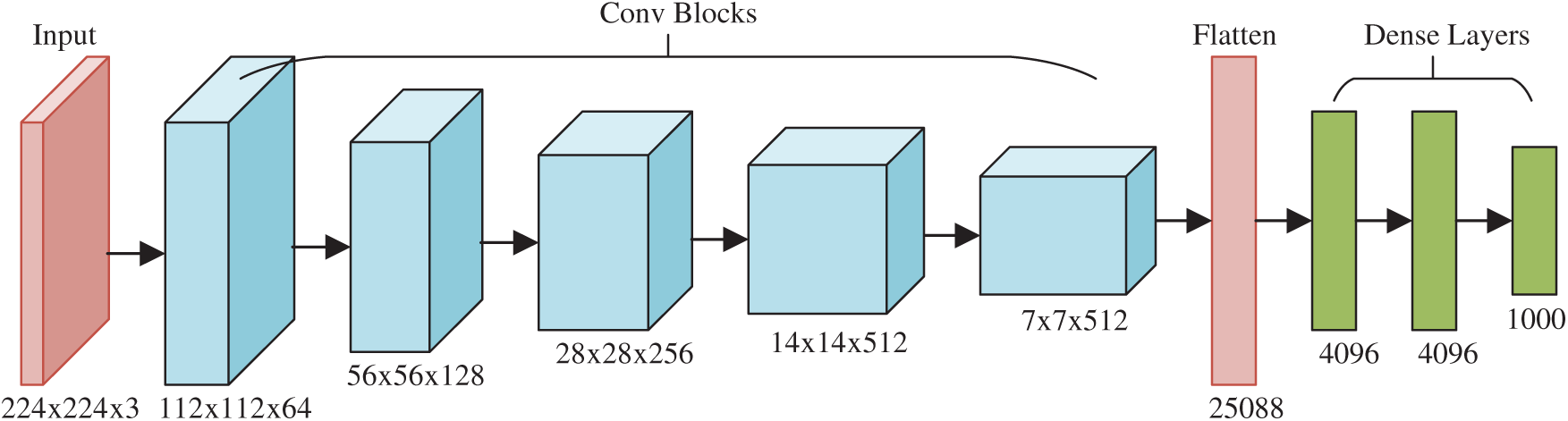
Figure 5: Structure of VGG-16

The 2nd CB is 2 × (128 3 × 3), 3rd CB 3 × (256 3 × 3), 4th CB 3 × (512 3 × 3), and 5th CB 3 × (512 3 × 3). Those generate the FMs with sizes of 56×56×128, 28×28×256, 14×14×512, and 7×7×512, respectively. Later, the FM of 5th CB is compressed into a vector of 25,088 neurons and delivered into three dense layers with the number of neurons of 4096, 4096, and 1000, respectively.

Inspired by VGG-16, this proposed DRAPNet network uses a small conv kernel other than a large kernel, and always uses 2x2 filters with a stride of 2 for pooling. Besides, both DRAPNet and VGG-16 employ repetitions of conv layers followed by pooling as a CB. They both use dense layers at the end. The structure of DRAPNet is adjusted by validation performance and itemized in Tab. 2, in which NWL represents the number of weighted layers, CH the configuration of hyperparameters.

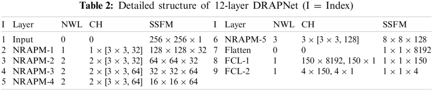
Compared to standard CNNs, the gains of DRAPNet include two points: (i) DRAPNet facilitates our model from overfitting by using the proposed NRAPM; (ii) DRAPNet is parameter-free. (iii) DRAPNet can be straightforwardly united with other enhanced network mechanisms, e.g., dropout, etc. Overall, we build this 12-layer DRAPNet. We have endeavored to incorporate more NRAPMs or more FCLs, which do not improve the functioning but adding more calculation loads.

Take a close-up of Tab. 2, the CH column in the top part has a format of a×[b×b,c], which stands of a repetitions of c filters with size of b×b. For the bottom part of Tab. 2, the d×e,f×g format in CH column means the weight matrix with size of d×e and bias vector with size of f×g. In the SSFM column of Tab. 2, the format of h×i×j stands for the spatial size of feature maps, where h,i,j represents height, width, and channel, respectively.

Tab. 3 itemizes the non-test, and test set for each class. The whole dataset TP comprises four non-overlapping categories TP={TP1,TP2,TP3,TP4}. For each class, the dataset is split into non-test set and test set TPk→{APk,BPk},k=1,2,3,4, where AP,BP mean the preprocessed non-test set, and preprocessed test set respectively

TP=def[TP1TP2TP3TP4]=def[AP⏟non-testBP⏟test]=def[AP1BP1AP2BP2AP3BP3AP4BP4].(9)

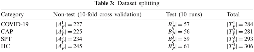
The experiment involves two stages. At Stage I, 10-fold cross-validation is utilized on the non-test set AP, to fix the best network structure and hyperparameters. The 18-way DA is utilized on the training set during 10-fold cross-validation.

Afterward, at Stage II, this DRAPNet model is trained using a non-test set AP as training set, and evaluated using a test set BP as test set. Again, 18-way DA is used on the training set. The algorithm run BR times with different initial seeds. Once combining the BR runs, we attain a summation of a test confusion matrix BM. Tab. 3 itemizes how the dataset is split, where |a| means the number of elements of the set a.

The ideal BM={bm(i,j),i=1,…,4,j=1,…,4} is a diagonal matrix with the appearance of

BMideal={bmideal(i,j)}=BR×[|BP1|0000|BP2|0000|BP3|0000|BP4|],(10)

where all the off-diagonal elements’ values are zero, i.e., bmideal(i,j)=0,∀i≠j, indicating no classification errors. In realistic AI models that make errors, the performance indicators are computed per class. For each class k=1,2,3,4, hat class label k is set as “positive”, and all other three classes fSD[(1,2,3,4),k] are “negative”, where fSD means the set difference function. Three performance indicators (sensitivity, precision, and F1 score) of class k are defined as:

Sen(k)=TP(k)/[TP(k)+FN(k)].(11)

Prc(k)=TP(k)/[TP(k)+FP(k)].(12)

F1(k)=[2×Prc(k)×Sen(k)]/[Prc(k)+Sen(k)].(13)

The test performance could be calculated over all four classes. The micro-averaged (MA) F1 (denoted as Fm) is harnessed, due to the slightly unbalance of our dataset

Fm=2×∑k=14⁡TP(k)∑k=14⁡TP(k)+FP(k)×∑k=14⁡TP(k)∑k=14⁡TP(k)+FN(k)∑k=14⁡TP(k)∑k=14⁡TP(k)+FP(k)+∑k=14⁡TP(k)∑k=14⁡TP(k)+FN(k).(14)

Lastly, gradient-weighted class activation mapping (Grad-CAM) is used to give clarifications on how this DRAPNet model renders the decision and which region it pays more attention to. Grad-CAM employs the gradient of the categorization score with regards to the convolutional features decided by our model. The FM of NRAPM-5 in Tab. 2 is harnessed for Grad-CAM.

5  Experiments, Results, and Discussions

Some common parameters are itemized in Tab. 4. The crop parameters are set as b1=b2=b3=b4=200. The size of final preprocessed image is WP=HP=256. The noisy density of SAPN is 0.05. The number of newly generated images of each DA is set as NI=30. We tested greater value of NI, however, it does not yield substantial advances on the validation set. The number of ways of DA is set to NW=18. For RAP, only 2 elements will be selected for each pooling region. The number of runs on the test set is set to BR=10. Besides, the operating system is Windows 10. The programming environment is MATLAB 2021a. GPU device is NVIDIA GeForce GTX1060.

5.1 Confusion Matrix of Proposed DRAPNet Model

Fig. 6 shows the confusion matrix of DRAPNet with 10 runs over the test set. Each row represents the number of samples in the true class, and each column represents the number of samples in the predicted class. The entry a(i,j) in this confusion matrix A stands for the number of cases in class i predicted as class j. Blue color (diagonal entries) and pink color (off-diagonal entries) represent the correct and incorrect observations, respectively.

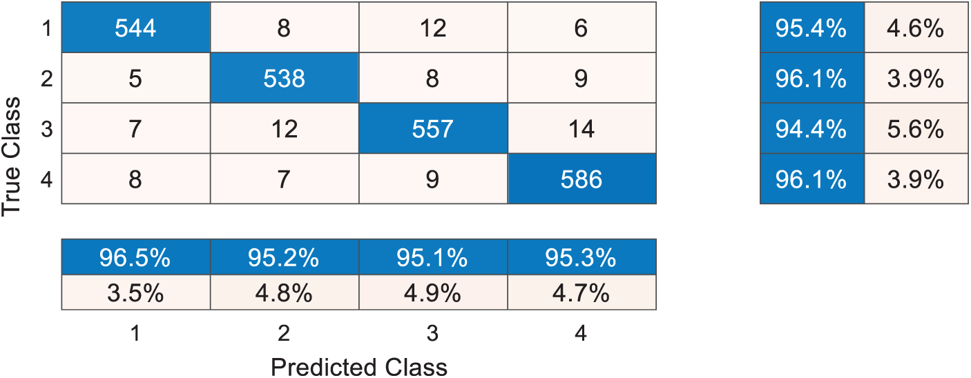
Figure 6: Confusion matrix with 10 runs over test set

Take a close-up to Fig. 6, the sensitivities of four classes are 95.44%, 96.07%, 94.41%, and 96.07%, respectively. The precisions of four classes are 96.45%, 95.22%, 95.05%, and 95.28%, respectively. The F1 scores of the four classes are not shown in Fig. 6, and their values are 95.94%, 95.64%, 94.73%, and 95.67%, respectively. The micro-averaged F1 is 95.49%.

5.2 Comparison of DRAPNet and Other Pooling Methods

Proposed DRAPNet is compared against the other four CNNs with various pooling techniques. Those five CNNs are SC-CNN, L2P-CNN, MP-CNN, and AP-CNN, respectively. Their description can be found in Section 4.2. Take SC-CNN as an example, it uses the same structure of DRAPNet but replaces RAP with SC. The results of 10 runs of those five methods over the test set are displayed in Tab. 5, where C represents class, (D1,D2,D3,D4) stands for the four classes.

There are in total 13 indicators, and we choose to use micro-averaged F1 as the main indicator since it takes the performances of all categories into consideration. The micro-averaged F1 scores of SC-CNN, L2P-CNN, MP-CNN, AP-CNN, and DRAPNet are 93.35%, 93.22%, 92.62%, 94.08%, and 95.49%, respectively. The reason why DRAPNet obtains the best micro-averaged F1 score is that RAP can prevent overfitting [15], which is the main shortcoming of max pooling. Meanwhile, L2P and AP average out the maximum activation values, that hurdle the performance of the corresponding L2P-CNN and AP-CNN models. For SC-CNN, it barely employs one-fourth of all knowledge of the input FM; and neglects the rest three-fourths of information; thus, its performance is not comparable to RAP.

5.3 Comparison to State-of-the-Art Approaches

This proposed DRAPNet method is compared with 8 state-of-the-art methods: WRE [4], RCBO [5], CSSNet [6], COVNet [7], CCD [8], FCONet [9], DeCovNet [10], VGG-16 [16]. All the experiments are implemented on the same test set by 10 runs. Comparison results are itemized in Tab. 6, where C represents class, (D1,D2,D3,D4) stands for the four classes. It is observed that the DRAPNet yields the greatest performance in terms of MA F1 and most of other indicators. The reason why this proposed DRAPNet performs the best is four reasons: (i) We use 18-way data augmentation to avoid overfitting, (ii) Our network is inspired by VGG, (iii) rank-based average pooling is used to replace traditional pooling, and (iv) Grad-CAM is used to provide explainability of our DRAPNet model.

5.4 Explainability

We take four samples (one sample per category) as examples, the raw images of those four pictures are shown in Figs. 7a–7d, their corresponding heatmaps are shown in Figs. 7e–7h, and the cognate manual delineation results are shown in Figs. 7i–7k. It is noteworthy there are no lesions within healthy subject images.

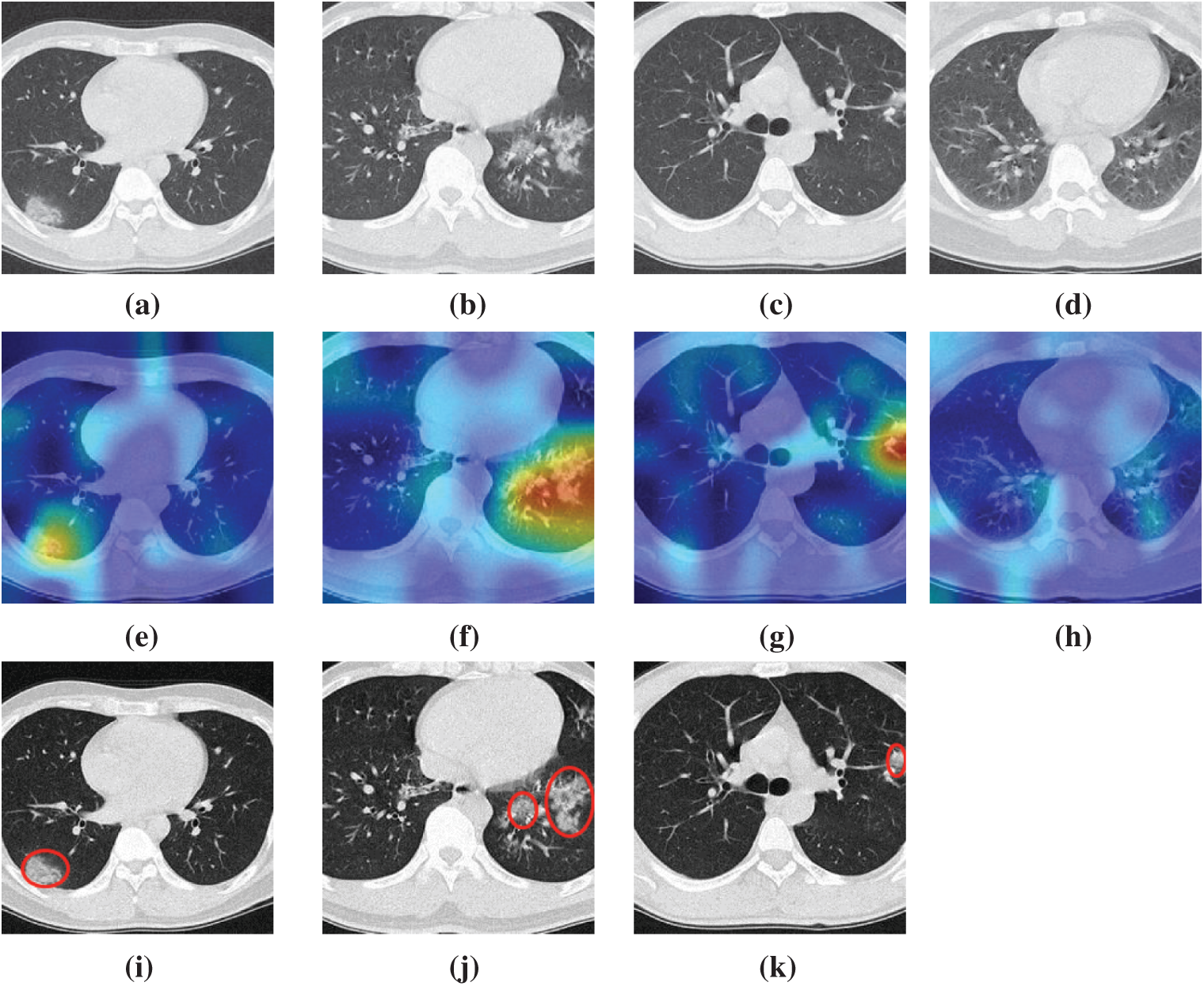
Figure 7: Heatmaps of three diseased samples and one healthy sample (a) A sample of COVID-19 (b) A sample of CAP (c) A sample of SPT (d) A sample of HC (e) Heatmap of COVID-19 (f) Heatmap of CAP (g) Heatmap of SPT (h) Heatmap of HC (i) Lesion of (a) (j) Lesion of (b) (k) Lesion of (c)

The FM of NRAPM-5 in DRAPNet is used to generate the heat maps by Grad-CAM. We can see from Fig. 7 that the heatmaps by this DRAPNet model and Grad-CAM are able to apprehend the diseased lesions efficiently and to ignore those non-lesion areas. Conventionally, AI is viewed as a “black box”, which hurdles its widespread use. Nevertheless, with the help of explainability of modern AI techniques, the radiologist and patients could gain assurances to this DRAPNet model, since the heat map gives a self-explanatory interpretation of how AI classifies COVID-19, CAP, SPT from healthy subjects.

6  Conclusion

This study proposes a DRAPNet that fuses four improvements: (a) proposed NRAPM module, (b) usage of rank-based average pooling; (c) multiple-way DA; and (d) explainability via Grad-CAM. These four improvements make our DRAPNet method yield better results than 8 state-of-the-art methods. The 10 runs on the test set demonstrate this DRAPNet model achieved a micro-averaged F1 score of 95.49%.

There are three aspects that can be improved in future studies: (a) Our DRAPNet method does not go through stringent clinical validation, so we will try to develop web apps based on the mode, and deploy our apps online, and invite radiologists and physicians to return feedbacks so we can continually improve it; (b) Data collection is still ongoing, and we expect to collect more images; (c) Segmentation techniques can be used within the preprocessing to remove unrelated regions prior to the DRAPNet model.

Funding Statement: This study is partially supported by the Medical Research Council Confidence in Concept Award, UK (MC_PC_17171); Royal Society International Exchanges Cost Share Award, UK (RP202G0230); Hope Foundation for Cancer Research, UK (RM60G0680); British Heart Foundation Accelerator Award, UK; Sino-UK Industrial Fund, UK (RP202G0289); Global Challenges Research Fund (GCRF), UK (P202PF11). We thank Dr. Hemil Patel for his help in English correction.

Conflicts of Interest: The authors declare that they have no conflicts of interest to report regarding the present study.

This work is licensed under a Creative Commons Attribution 4.0 International License, which permits unrestricted use, distribution, and reproduction in any medium, provided the original work is properly cited.