DOI:10.32604/cmc.2022.020143
| Computers, Materials & Continua DOI:10.32604/cmc.2022.020143 | |
| Article |
Generating Synthetic Data to Reduce Prediction Error of Energy Consumption
Department of Computer Engineering, Jeju National University, Jeju-si, Korea
*Corresponding Author: Yung-Cheol Byun. Email: ycb@jejunu.ac.kr
Received: 11 May 2021; Accepted: 18 June 2021
Abstract: Renewable and nonrenewable energy sources are widely incorporated for solar and wind energy that produces electricity without increasing carbon dioxide emissions. Energy industries worldwide are trying hard to predict future energy consumption that could eliminate over or under contracting energy resources and unnecessary financing. Machine learning techniques for predicting energy are the trending solution to overcome the challenges faced by energy companies. The basic need for machine learning algorithms to be trained for accurate prediction requires a considerable amount of data. Another critical factor is balancing the data for enhanced prediction. Data Augmentation is a technique used for increasing the data available for training. Synthetic data are the generation of new data which can be trained to improve the accuracy of prediction models. In this paper, we propose a model that takes time series energy consumption data as input, pre-processes the data, and then uses multiple augmentation techniques and generative adversarial networks to generate synthetic data which when combined with the original data, reduces energy consumption prediction error. We propose TGAN-skip-Improved-WGAN-GP to generate synthetic energy consumption time series tabular data. We modify TGAN with skip connections, then improve WGAN-GP by defining a consistency term, and finally use the architecture of improved WGAN-GP for training TGAN-skip. We used various evaluation metrics and visual representation to compare the performance of our proposed model. We also measured prediction accuracy along with mean and maximum error generated while predicting with different variations of augmented and synthetic data with original data. The mode collapse problem could be handled by TGAN-skip-Improved-WGAN-GP model and it also converged faster than existing GAN models for synthetic data generation. The experiment result shows that our proposed technique of combining synthetic data with original data could significantly reduce the prediction error rate and increase the prediction accuracy of energy consumption.
Keywords: Energy consumption; generative adversarial networks; synthetic data; time series data; TGAN; WGAN-GP; TGAN-skip; prediction error; augmentation
Energy preservation is the source of economic development and plays a significant role in social progress and residential environmental evolution. Countries all over the world are rapidly shifting towards renewable and nonrenewable energy sources. Energy consumption forecasting is an approach to predict the future consumption of energy so that energy companies can plan and design policies for the future more efficiently. This also helps in eliminating financial loss for the industry. Machine learning and deep learning prediction models or techniques are being widely used for power load forecasting. Load forecasting generally predicts the total system load per hour, day, week, or month for every specific geographic location. Load data for energy consumption are time series tabular data. There exist well-known machine learning algorithms to predict energy forecasts, but most of the time, the prediction error rates are high. There can be a substantial financial loss even if the predicted load value differs from the actual load value by few points. Previously, we have used multiple ensemble models to predict energy consumption [1,2]. But, we could observe that although we had a large dataset, the prediction error rate was high for the days having less record. For e.g., days when there was any natural disaster like typhoon, earthquake or when there was some special holiday, etc. So, to reduce prediction error, it is important to balance the variation of records which can be done by generating records of less frequency. Synthetic generation of data and augmentation can solve the above issue of data scarcity. Synthetic data can be referred to as artificial data that replicates the statistical characteristics of real data. Augmentation is also a process by which we can increase the records of the existing dataset. Synthetic data generation is a trending process and the latest models used for generating superior quality of synthetic data are variational autoencoders and generative adversarial networks (GAN). In this paper, we propose augmentation and synthetic time series data generation techniques that can generate new tabular data, which reduces energy consumption prediction error and enhances the accuracy when combined with original data. The main contribution of this paper is summarized below:
• We proposed different augmentation techniques for time series tabular data.
• In this work, we proposed tabular GAN (TGAN) with skip connections (TGAN-skip) and adapted improved version of Wasserstein GAN with gradient penalty (WGAN-GP) architecture for training TGAN-skip to generate synthetic tabular data. We named the model as TGAN-skip-Improved-WGAN-GP which could enhance the performance by reducing convergence time and eliminating mode collapse problem.
• For augmentation we experimented with multiple random transformation techniques and discriminative guided warping of data that is based on dynamic time warping (DTW) and shape-DTW.
The integration of renewable energy and nonrenewable energy into electric grids increases energy demand requirements [3]. The power load historical data are a sample of ordered collections which is recorded as specific time intervals. This makes them time-series records. The traditional energy sources keep pace with wind and solar energy. At the same time, due to positive aspects of renewable energy such as low-carbon, stable, reliable, and environmentally friendly the consumers upgrade renewable energy demands [4]. Chengquan et al. [5], presented the two-tier management system based on the degradation of the cost model with the hybrid energy system. This system overcomes the cost of low operations and takes them into energy fluctuation account.
Shapi et al. [6] defined Microsoft Azure cloud-based machine learning platform for predicting energy consumptions in building energy management system (BEMS). They proposed that cloud based models for prediction would not depend on the hardware it’s running on and would be able to handle different distributions of energy consumption. Bourhnane et al. [7] used artificial neural networks along with genetic algorithms for energy consumption prediction and scheduling. They express in their paper that prediction models could not produce high accuracy result due to the lack of data. Wang et al. [8] proposed a stacking model to forecast building energy consumption. This model integrates advantages of multiple base prediction algorithms and forms meta-features to discover spatial and structural angle of the dataset. Machine learning has been widely used in generating synthetic patient data. Most commonly used models are probabilistic models, classification-based imputation models and generative adversarial networks (GAN) [9].
Jaeuk et al. [10] proposed the solution for the data shortage problem based on two-stage data generation, which effectively extracts the input and output variables for short-term load forecasting. The first step is to extract the virtual calendar and the related data to temperature as input for GAN and CTGAN. The second step is to load the electric data as an input for the deep learning regression model. The process finalizes by generating actual data based on applying a regression model on the generated dataset. Kavousi et al. [11] presented the various machine learning techniques such as Artificial Neural Network (ANN) and autoregressive model for the wavelet transform. This process is used to make the correlation of the functions for the time series electric load in terms of stationary and non-stationary behaviors. The energy consumption data has been obtained on a half-hourly basis.
Chenlu et al. [12], proposed the prediction of a parallel scheme applying few amounts of data for generating the artificial data based on GAN. The applied dataset is containing the original and synthetic type of data using the machine learning forecasting models. Kang et al. [13] presented forecasting of the stock market using GAN based on the LSTM and MLP machine learning models. The train set contains the daily stock data, which this process shows the improvement of forecasting accuracy in this system.
Rezagholiradeh et al. [14] applied GAN to overcome the problem of regression. The GAN structure in this process generates the train data and carries out the forecasting. This system becomes successful in reducing the errors of the proposed model. MedGAN [15] processing is based on an auto-encoder, but it is available for numeric and binary data types. The design of this system doesn’t support the various type of dataset, and to process the different data types, different models are required [16]. The numerical data is well fitted with the TableGAN and VEEGAN, but there is a problem for categorical data [17] in terms of collapse mode. GAN is a successful image generation method, but the training is not stable and straightforward [18].
In this section, we explain our proposed approach on reducing prediction error of energy consumption by generating synthetic time series data. Through this work, we demonstrate that machine learning models when trained by combining original time series energy consumption data with synthetic data can reduce the prediction error rate to a good extent as compared to using only original real time data to train the models. In Fig. 1, we have presented the overview of our proposed methodology. The proposed approach has been divided into four stages. As input, we have considered real time energy consumption data of Jeju province in South Korea. The next stage is the preprocessing stage, where we prepare the data according to different model requirement. First, we train prediction models by using original data and then extract the data that has absolute error more than four. This data is then used as input to the augmentor or GAN synthesizer. After preprocessing comes the augmentation stage, where we perform various traditional augmentation techniques along with synthetic generation of data using different variations of generative adversarial networks. We propose that the architecture of an improved version of WGAN-GP can be adapted by TGAN with skip connections to generate synthetic energy consumption time series data. We name our proposed model as TGAN-skip-Improved-WGAN-GP. In the last stage, we combine the original data with the augmented or synthetic data generated by each model. We then evaluate the energy consumption prediction error with and without combining synthetic data with the original data. In the result section we assess the quality of synthetic data generated by our proposed model compared to augmented or synthetic data generated by other models. We also compare the prediction accuracy, mean error and maximum error with and without using synthetic data.

Figure 1: Overview of the proposed approach
2.1 Energy Consumption Time Series Tabular Data
For our experiment, we have acquired real time energy and weather data of Jeju Island from Jeju Energy Corporation. Korea Power Exchange (KPE) and Korea Electric Power Corporation (KEPC) are the two main sources of electricity and renewable energy in South Korea. The three primary sources of renewable energy for these organizations are obtained through contractless small-sized behind the meter energy generator, photovoltaic solar energy generator and wind power energy generator. There are five weather stations in Jeju Island that acquires data from all over the Island.
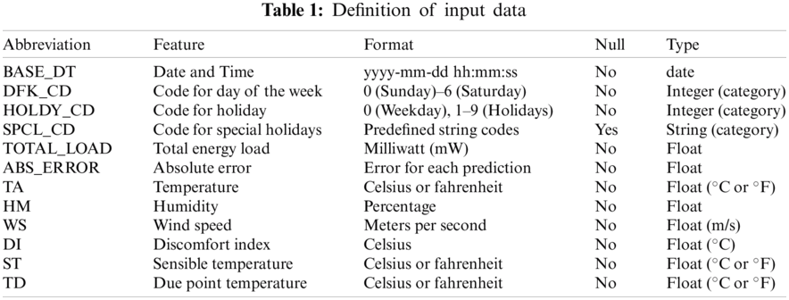
We used energy consumption data of Jeju Island, South Korea dated from January 2012 to August 2018 to train our model. The time series energy consumption tabular data has been obtained on a half-hourly basis. As a result, we received 48 entries per day of energy load. In Tab. 1, we define the columns of the energy data and their properties.
In the preprocessing stage, we perform different operations such as segregation of fields, data cleaning, null value removal, encoding and data extraction. The tabular time series energy data is prepared according to the requirement of the augmentation or GAN model. Firstly, we replace NaN values with zero. From the BASE_DT column, we extract year, month, day, hour, minutes and seconds. For SPCL_CD, we encode the string codes to categorical format. Initially, with the original raw data, we apply a hybrid ensemble model consisting of CatBoost, Gradient Boost and Multilayer Perceptron to perform energy consumption prediction. For every row in the tabular data, we compare the original energy consumption with the predicted energy consumption value. We then compute the absolute error for each prediction. We sort the ABS_ERROR field in descending order and extract the data that has an error value of more than four. For augmentation and synthetic data generation, we experimented with different variations of data such as training the GAN synthesizer on the whole original data to generate new synthetic energy consumption data. We also experimented by synthesizing data that has an ABS_ERROR greater than four. We selected different values of ABS_ERROR to extract the energy consumption data which was further used to generate augmented and synthetic data to test the prediction model. We observed that not every augmented or synthetic data can reduce the prediction error rate. So, in our work, we did a vast experimentation with multiple combination of synthetic data and models. In this paper, we have proposed a generative adversarial networks-based model to generate synthetic data which when combined with original data reduced the prediction error rate to a great extent. We have also tested our proposed model with other publicly available datasets to verify the efficiency of the model when used in different scenarios. Different preprocessing techniques have been applied to different datasets as required by specific augmentation and GAN models.
2.3 Augmentation Through Random Transformation and Discriminative Guided Warping
Data augmentation is a familiar process in image processing. A lot of techniques for time series data augmentation are borrowed from data augmentation of images commonly termed as random transformations. Random transformation includes jittering, rotation, scaling, cropping, magnitude warping, time warping and many other methods. Data augmentation through random transformation uses specific transformation function to generate pattern D′, where D is a sequence with T number of time steps denoted as D = D1, …, Dt, …, DT and where every element Dt can be univariate or multivariate. Random transformation of time series data can be divided into three categories namely magnitude domain transformation, time domain transformation and frequency domain transformation. Magnitude domain transformation refers to the transformation performed on the values of the time series tabular data. In time domain transformation, the transformation is applied on the time axis whereas in frequency domain transformation periodic signals are considered to be transformed. In this paper, we have used some of the transformation techniques from each domain. Below, we explain the random transformation-based data augmentation techniques we have used in this paper.
• Jittering–Jittering [19] is the transformation process which has been used to add noise in our energy consumption time series tabular data. We define jittering as in Eq. (1)
where λ is the Gaussian noise that is added for every element Dt at each time step t. Including noise has shown to induce generalization and enhance the performance of neural networks. Through jittering the time series data created new energy consumption data patterns that are different from the original data with respect to addition of noise.
• Rotation–Rotation transformation [20] in the energy consumption time series data can be defined as in Eq. (2)
where R denoted the element-wise random rotation matrix for multivariate time series data and for univariate time series data it represents random flipping.
• Scaling–Scaling adds a random scalar value [21] in the energy consumption data which increases or decreases the magnitude of each element. Scaling is described with below Eq. (3)
where Ω is the scaling parameter that is determined by the Gaussian distribution Ω ∼ N (1, σ2) and σ is the hyperparameter. Scaling does not enlarge the time series data but only increases or decreases the magnitude of elements.
• Magnitude Warping–Through magnitude warping [22], we multiply the magnitude of energy consumption times series data with a smoothed curve and can be defined as in Eq. (4)
where M1, … , Mt, … , MT is the sequence incorporated from the cubic spline with knots taken from a distribution N (1, σ2 ), where σ is the hyperparameter. Magnitude warping helps in adding small fluctuations in the time series data which broadens the prospect of the dataset.
• Time Warping–Time warping generally warps in the temporal dimension through a random smooth curve produced by the cubic spline with knots at the random magnitude. The augmented data obtained through time warping can be defined as in Eq. (5)
where T(·) represents the warping function based on the curve defined by the cubic spline.
• SPAWNER–Suboptimal Warped Time Series Generator (SPAWNER) performs augmentation of energy consumption data through suboptimal time warping [23]. SPAWNER averages aligned patterns and can create unlimited new time series energy consumption data.
• Discriminative Guided Warping with Dynamic Time Warping (DGW-D) and Discriminative Guided Warping with shapeDTW (DGW-SD)–Lets us consider two time series denoted as a = a1, … , ax, … , aX and b = b1, … , by, …, bY with sequence length X and Y. Given sequence a and b, dynamic time warping (DTW) can determine the global distance between them where element ax and by can represent univariate or multivariate time series data. Dynamic time warping is useful for measuring an optimized distance for time series data. It matches the time series elements non-linearly in the time dimension by warping the sequences to find the minimal path between element-wise time series using dynamic programming.
This minimal distance is known as the warping path which acts as a mapping between time steps of one sequence and another. Guided warping provides guidance for time warping based on a reference pattern and uses the dynamic alignment function of DTW to warp the elements in the time domain. There are two variants of guided warping random guided warping or discriminative guided warping (DGW). DGW-D uses a discriminative teacher as the reference pattern for guided warping. On the other hand, shapeDTW uses shape-descriptors to warp sample patterns within the sequence which helps in maintaining the original features of the energy time series data while generating unlimited related new samples. Fig. 2 represents the overview of DGW presented in work [24] which we followed to select the discriminative teacher and to improve the energy consumption time series data augmentation with shape descriptors.

Figure 2: Discriminative guided warping (DGW)
2.4 Generative Adversarial Networks for Generating Synthetic Energy Consumption Data
Since the introduction of generative adversarial networks in 2014 by Goodfellow et al. [25], it has been widely used in the generation of new and vast image, video and audio datasets. GAN has been used in multiple fields to augment image data, tabular data and signal data. Also, GAN is well known for generating synthetic data that can be used to train machine learning algorithms to improve the performance of the model by increasing accuracy and reducing error rate. GAN is a machine learning framework which consists of two neural networks known as generator (G) and discriminator (D) which competes against each other in a zero-sum game. The flow of GAN architecture is shown in Fig. 3. The generator receives random input noise NZ (Z) and retains the original data distribution DZ over data x. The generator outputs samples that serves as input to the discriminator along with the original data distribution. Function of discriminator is to differentiate generated data from real data. So, in the zero-sum game the generator tries to fool the discriminator and the discriminator tries to correctly distinguish between real and generated data. Through the computation and feedback of the generator and discriminator loss the GAN tries to improve its performance. The generator’s task is to minimize log(1 − D(G(Z))) where the minmax function is defined as in Eq. (6).

Figure 3: Architecture of generative adversarial networks (GAN)
In this paper, we propose a GAN model that combines the architecture of tabular GAN (TGAN) and Wasserstein GAN with gradient penalty (WGAN-GP). The proposed model is termed as TGAN-skip-Improved-WGAN-GP where we modify the tabular GAN with skip connections, improve the training of WGAN-GP with a consistency term and use the architecture of improved WGAN-GP to train TGAN-skip model. Our proposed model can generate synthetic energy consumption time series tabular data which when used for prediction, reduces the prediction error rate to a considerable amount and increases the accuracy of the prediction model. First, we perform data transformation where we define meaningful representation of continuous and categorical values. Then the data is processed through TGAN-skip-Improved-WGAN-GP model and further inverse transformation is performed, after which final synthetic energy consumption time series tabular data is generated. Machine learning models require meaningful representation of real data which is achieved through data transformation. Data transformation performs normalization for continuous values by transforming the continuous values within 0 and 1. Whereas data transformation standardizes the continuous values by transforming the data to obtain a mean value of 0 and a standard deviation of 1. In our experiment we have performed standardization of the original data for continuous values and used embedding techniques for data transformation of categorical values which converts the large vectors into small dimensional space vectors and preserves the semantic relationship.
Tabular GAN was introduced in the year 2018 [26] and since then, it has been widely used for generating synthetic tabular data of different fields and for various applications. In Fig. 4 we present the difference between TGAN and our proposed TGAN with skip connections architecture. Including skip connections in the TGAN eradicates vanishing gradient problem and also reduces the convergence time for the generator. The TGAN-skip architecture conserves the activation of high magnitude by initiating prompt activation and allowing them to skip in-between dense layers which results in preserving the old information. In the TGAN-skip architecture we use long short-term memory (LSTM) in the generator network architecture and multilayer perceptron for the discriminator network as shown in Figs. 5a and 5b. We have modeled the generator to produce categorical values in one step and the continuous values in two steps. First, the value scalar VSi is generated for continuous variables, after which we generate the cluster vector CVi. The probability distribution Pi is computed for categorical variables for each label. R representing random variable along with context vector Ci which is attention-based and previous hidden vector Hi or embedding vector
where

Figure 4: Architectural difference between TGAN and TGAN-skip

Figure 5: (a) Architecture of the generator, (b) Architecture of the discriminator
Wasserstein GAN (WGAN) was introduced to improve the training and eliminate the flaws of Vanilla GAN [27]. Later, Gulrajani et al. [28], proposed improved WGAN known as WGAN-GP where GP stands for gradient penalty which would comply the constraint of 1-Lipschitz and would remove the requirement for clipping. WGAN-GP improved WGAN by introducing a new loss that would combine the gradient penalty loss with the original critic loss as defined in Eqs. (8) and (9)
where dn and Gn represents data distribution and generator distribution and
we add to the value function of WGAN, a consistency term CT as defined in Eq. (11) to penalize the infringement occurred in Eq. (10).
Defining the consistency term and using the improved version of WGAN-GP architecture for TGAN-skip instead of normally used Vanilla GAN training architecture, reduced the loss of the discriminator and enhanced the generator performance. This helped in avoiding mode collapse problem and stagnation scenario and also our proposed model TGAN-skip-Improved-WGAN-GP, converged much faster. For implementing improved-WGAN-GP architecture in TGAN-skip model, we adapted the consistency term in WGAN-GP and the loss function. We also modified the batch normalization to layer normalization in the discriminator and removed sigmoid activation from last layer. Thus, the discriminator was trained for more iterations. At last, we perform inverse transformation to generate more meaning to the initially transformed dataset by transforming discrete values to multinomial distribution and continuous variables to scalar values. Our proposed architecture could produce better quality of synthetic data as presented in the evaluation and result section.
We evaluated our proposed model based on the synthetic and augmented data quality, prediction accuracy and error rates. For every augmented or synthesized data, we computed the mean correlation coefficient, mean absolute error, root mean square error, percent root mean square difference, Fréchet distance, and mirror column association. Also, we have evaluated different variations of augmented and synthetic data on our prediction model. We presented the prediction accuracy, mean error and the maximum error for every synthetic or augmented data tested on our prediction model.
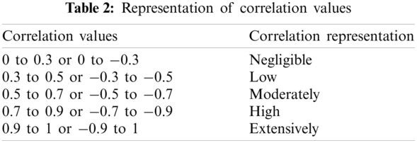
For assessing the synthetic data, we compute the correlation coefficient of the synthetic data with the original data by measuring Pearson’s correlation coefficient that ranged from −1 to 1. The depiction of the correlation values is shown in Tab. 2 where direct relationship is represented by a positive value, inverse relation is depicted by a negative value and zero represents no relationship. Pearson’s correlation coefficient PCoef can be defined as in Eq. (12), where original data is represented by OriData and synthetic data is represented by SynData.
Mean absolute error (MAE) is the measure of absolute error between the synthetic data and the original data as defined by Eq. (13).
Root mean square error (RMSE) quantifies the stability and measures how the synthetic data is different from the original data as defined by Eq. (14).
3.3 Percent Root Mean Square Difference
Percent Root Mean Square Difference (PRD) measures the distortion between the synthetic and the original signals as defined by Eq. (15).
Fréchet Distance is used for finding the similarity in ordering and also to find the location of points along the curve. If OriDatai = O1, O2, O3, … , Oi is order of points in original data curve and SynDataj = S1, S2, S3, … , Sj is for synthetic data curve, we can compute the sequence length ||l|| as defined in Eq. (16) [26]
where Euclidean distance is defined by l and
Mirror column association is used find the rate of association between each column from the synthetic and original dataset. Greater the value, greater is the association, representing better performance.
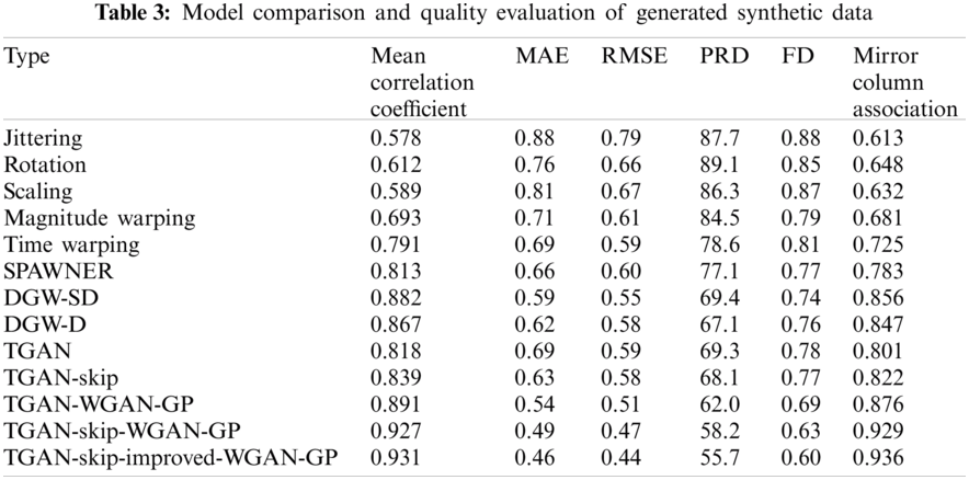
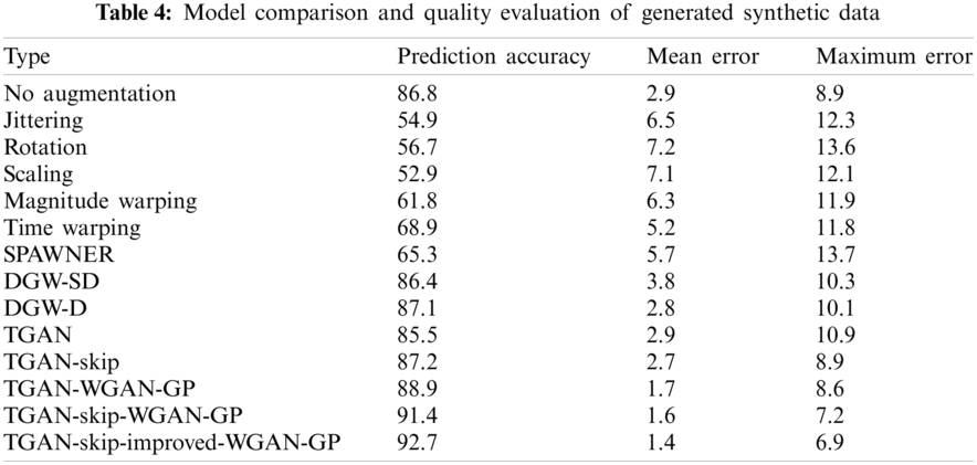
Tab. 3 represents the quality of the synthetic and augmented data generated by different models and techniques. As we can see from Tab. 3, that our proposed model achieves better result as compared to existing models with an association value of 0.936 and also reduces the error to a good extent. In Tab. 4, we present the prediction accuracy, mean error and maximum error which depicts that when the synthetic data generated by our proposed model is combined with the original data, prediction accuracy is increased and error rate is decreased.
3.6 Computation of Mean and Standard Deviation of Original and Synthetic Data
We present the visual representation of the mean and standard deviation of every column. The diagonal line represents the original data, so the closer the plotted points to the diagonal line, the better is the correlation between the original and the synthetic data. In Fig. 6 we have compared the mean and standard deviation produced by DGW-SD, TGAN-WGAN-GP and our proposed model TGAN-skip-Improved-WGAN-GP. Result depicts that the synthetic data generated by TGAN-skip-improved-WGAN-GP is more correlated to the original data as compared to other existing models which concludes that our proposed model achieves better results and can be used for generating synthetic time series tabular data.

Figure 6: Comparison of mean and standard deviation of different models
In this paper, we propose that prediction accuracy and error rate can be improved if we try to balance the dataset. Many a times, we receive large amount of data, but each case in the dataset are not always well distributed, or the data is not uniform. In our case, we had large amount of entries in the energy consumption data, but when we tried to use prediction algorithm, the error rate was more. This was due to the fact that there were less entries for days with special events, holidays, natural calamities etc. So, in this paper we experimented and proposed that augmenting or generating synthetic data and combining them with the original data to balance the dataset can reduce prediction error and enhance the prediction accuracy.
We divided our work into four stages. In the first stage, we receive the energy consumption time series tabular data as input. In the second stage, we preprocess the data according to the requirement of different GAN models and augmentation method. In the third stage, for augmentation, we perform random transformation and discriminative guided warping. In random transformation, we experiment our dataset with jittering, rotation, scaling, magnitude warping, time warping, SPAWNER. In discriminative guided warping, we augment the data with dynamic time warping and shape DTW. We then propose a generative adversarial networks-based model named as TGAN-skip-Improved-WGAN-GP which modifies TGAN with skip connections and then enhances the training of TGAN-skip with improved WGAN-GP architecture. We improve WGAN-GP architecture by defining a consistency term. We experiment our datasets with various other GAN models. In the result section we compute the prediction accuracy, mean error and maximum error when different augmented and synthetic datasets are used with the original data. We also measure the quality of the generated data through MAE, RMSE, PRD, FD, mirror column association and mean correlation coefficient. We also visually presented the mean and standard deviation of generated data and original data from different augmentation and GAN models. Results show that generated data from our proposed model TGAN-skip-Improved-WGAN-GP when combined with original data can significantly reduce the prediction error rate and improve the prediction accuracy as compared to using only original data to predict energy consumption.
Funding Statement: This research was financially supported by the Ministry of Small and Medium-sized Enterprises (SMEs) and Startups (MSS), Korea, under the “Regional Specialized Industry Development Program (R&D, S3091627)” supervised by Korea Institute for Advancement of Technology (KIAT).
Conflicts of Interest: The authors declare that they have no conflicts of interest to report regarding the present study.
1. P. W. Khan and Y. C. Byun, “Genetic algorithm based optimized feature engineering and hybrid machine learning for effective energy consumption prediction,” IEEE Access, vol. 8, pp. 196274–196286, 2020. [Google Scholar]
2. P. W. Khan, Y. C. Byun, S. J. Lee, D. H. Kang, J. Y. Kang et al., “Machine learning-based approach to predict energy consumption of renewable and non renewable power sources,” Energies, vol. 13, no. 18, pp. 4870–4886, 2020. [Google Scholar]
3. F. R. Badal, P. Das, S. K. Sarker and S. K. Das, “A survey on control issues in renewable energy integration and microgrid,” Protection and Control of Modern Power Systems, vol. 4, no. 1, pp. 1–27, 2019. [Google Scholar]
4. H. M. Marczinkowski, P. A. Østergaard and S. R. Djørup, “Transitioning island energy systems-local conditions, development phases, and renewable energy integration,” Energies, vol. 12, no. 18, pp. 3484–3504, 2019. [Google Scholar]
5. J. Chengquan, P. Wang, L. Goel and Y. Xu, “A two-layer energy management system for microgrids with hybrid energy storage considering degradation costs,” IEEE Transactions on Smart Grid, vol. 9, no. 6, pp. 6047–6057, 2017. [Google Scholar]
6. M. K. M. Shapi, N. A. Ramli and L. J. Awalin, “Energy consumption prediction by using machine learning for smart building: Case study in Malaysia,” Developments in the Built Environment, vol. 5, no. 10, pp. 100037, 2021. [Google Scholar]
7. S. Bourhnane, M. R. Abid, R. Lghoul, K. Z. Dine, N. Elkamoun et al., “Machine learning for energy consumption prediction and scheduling in smart buildings,” SN Applied Sciences, vol. 2, no. 2, pp. 1–10, 2020. [Google Scholar]
8. R. Wang, S. Lu and W. Feng, “A novel improved model for building energy consumption prediction based on model integration,” Applied Energy, vol. 262, pp. 114561–114575, 2020. [Google Scholar]
9. A. Goncalves, P. Ray, B. Soper, J. Stevens, L. Coyle et al., “Generation and evaluation of synthetic patient data,” BMC Medical Research Methodology, vol. 20, pp. 1–40, 2020. [Google Scholar]
10. M. Jaeuk, S. Jung, S. Park and E. Hwang, “Conditional tabular GAN-based two-stage data generation scheme for short-term load forecasting,” IEEE Access, vol. 8, pp. 205327–205339, 2020. [Google Scholar]
11. F. A. Kavousi and M. R. A. Zadeh, “A hybrid method based on wavelet, ANN and ARIMA model for short-term load forecasting,” Journal of Experimental & Theoretical Artificial Intelligence, vol. 26, no. 2, pp. 167–182, 2014. [Google Scholar]
12. T. Chenlu, C. Li, G. Zhang and Y. Lv, “Data driven parallel prediction of building energy consumption using generative adversarial nets,” Energy and Buildings, vol. 186, no. 6, pp. 230–243, 2019. [Google Scholar]
13. Z. Kang, G. Zhong, J. Dong, S. Wang and Y. Wang, “Stock market prediction based on generative adversarial network,” Procedia Computer Science, vol. 147, pp. 400–406, 2019. [Google Scholar]
14. M. Rezagholiradeh and M. A. Haidar, “Reg-GAN: Semi-supervised learning based on generative adversarial networks for regression,” in Int. Conf. on Acoustics, Speech, and Signal Processing, Calgary, AB, Canada, pp. 2806–2810, 2018. [Google Scholar]
15. C. Edward, S. Biswal, B. Malin, J. Duke, W. F. Stewart et al., “Generating multi-label discrete patient records using generative adversarial networks,” in Machine Learning for Healthcare Conf., Boston, Massachusetts, USA, pp. 286–305, 2017. [Google Scholar]
16. B. Bauke, A. D. Vries, E. Marchiori and Y. Hille, “On the generation and evaluation of tabular data using GANs,” Ph.D. Dissertation Master’s Thesis. Radboud University, Nijmegen, 2019. [Google Scholar]
17. L. Xu, M. Skoularidou, A. C. Infante and K. Veeramachaneni, “Modeling tabular data using conditional GAN,” in Advances in Neural Information Processing Systems, Vancouver, BC, Canada, pp. 7335–7345, 2019. [Google Scholar]
18. Y. Jinsung, L. N. Drumright and M. V. D. Schaar, “Anonymization through data synthesis using generative adversarial networks (ADS-GAN),” IEEE Journal of Biomedical and Health Informatics, vol. 24, no. 8, pp. 2378–2388, 2020. [Google Scholar]
19. T. T. Um, F. M. J. Pfister, D. Pichler, S. Endo, M. Lang et al., “Data augmentation of wearable sensor data for Parkinson’s disease monitoring using convolutional neural networks,” in Int. Conf. on Multimodal Interaction, Glasgow, Scotland, pp. 216–220, 2017. [Google Scholar]
20. K. M. Rashid and J. Louis, “Window-warping: A time series data augmentation of IMU data for construction equipment activity identification,” in Proc. of the Int. Symp. on Automation and Robotics in Construction, Banff Alberta, Canada, vol. 36, pp. 651–657, 2019. [Google Scholar]
21. L. Tran and D. Choi, “Data augmentation for inertial sensor-based gait deep neural network,” IEEE Access, vol. 8, pp. 12364–12378, 2020. [Google Scholar]
22. N. T. Son, S. Stueker, J. Niehues and A. Waibel, “Improving sequence-to-sequence speech recognition training with on-the-fly data augmentation,” in IEEE Int. Conf. on Acoustics, Speech and Signal Processing, Barcelona, Spain, pp. 7689–7693, 2020. [Google Scholar]
23. K. Kamycki, T. Kapuscinski and M. Oszust, “Data augmentation with suboptimal warping for time-series classification,” Sensors, vol. 20, no. 1, pp. 98–113, 2019. [Google Scholar]
24. B. K. Iwana and S. Uchida, “Time series data augmentation for neural networks by time warping with a discriminative teacher,” in Int. Conf. on Pattern Recognition, Milano, Italy, pp. 3558–3565, 2020. [Google Scholar]
25. I. Goodfellow, J. P. Abadie, M. Mirza, B. Xu, D. W. Farley et al., “Generative adversarial nets,” Advances in Neural Information Processing Systems, vol. 27, pp. 2672–2680, 2014. [Google Scholar]
26. L. Xu and K. Veeramachaneni, “Synthesizing tabular data using generative adversarial networks,” Computing Research Repository, vol. abs/1811, 2018. [Google Scholar]
27. M. Arjovsky, S. Chintala and L. Bottou, “Wasserstein gan,” in Proc. of the 34th Int. Conf. on Machine Learning, Sydney, Australia, 2017. [Google Scholar]
28. I. Gulrajani, F. Ahmed, M. Arjovsky, V. Dumoulin and A. C. Courville, “Improved training of wasserstein gans,” in Proc. of the 31st Int. Conf. on Neural Information Processing Systems, Long Beach, CA, USA, pp. 5767–5777, 2017. [Google Scholar]
29. X. Wei, B. Gong, Z. Liu, W. Lu and L. Wang, “Improving the improved training of wasserstein gans: A consistency term and its dual effect,” in 6th Int. Conf. on Learning Representations, Vancouver, BC, Canada, 2018. [Google Scholar]
30. D. Hazra and Y. C. Byun, “SynSigGAN: Generative adversarial networks for synthetic biomedical signal generation,” Biology, vol. 9, no. 12, pp. 441–461, 2020. [Google Scholar]
31. F. Zhu, F. Ye, Y. Fu, Q. Liu and B. Shen, “Electrocardiogram generation with a bidirectional LSTM-CNN generative adversarial network,” Scientific Reports, vol. 9, no. 1, pp. 1–11, 2019. [Google Scholar]
 | This work is licensed under a Creative Commons Attribution 4.0 International License, which permits unrestricted use, distribution, and reproduction in any medium, provided the original work is properly cited. |