Computers, Materials & Continua DOI:10.32604/cmc.2022.020261
Article

Improved KNN Imputation for Missing Values in Gene Expression Data

Phimmarin Keerin1 and Tossapon Boongoen2,*

1Faculty of Science and Technology, Pibulsongkram Rajabhat University, Thailand
2Center of Excellence in Artificial Intelligence and Emerging Technologies, School of Information Technology, Mae Fah Luang University, Chiang Rai 57100, Thailand
*Corresponding Author: Tossapon Boongoen. Email: tossapon.boo@mfu.ac.th
Received: 17 May 2021; Accepted: 12 July 2021

Abstract: The problem of missing values has long been studied by researchers working in areas of data science and bioinformatics, especially the analysis of gene expression data that facilitates an early detection of cancer. Many attempts show improvements made by excluding samples with missing information from the analysis process, while others have tried to fill the gaps with possible values. While the former is simple, the latter safeguards information loss. For that, a neighbour-based (KNN) approach has proven more effective than other global estimators. The paper extends this further by introducing a new summarization method to the KNN model. It is the first study that applies the concept of ordered weighted averaging (OWA) operator to such a problem context. In particular, two variations of OWA aggregation are proposed and evaluated against their baseline and other neighbor-based models. Using different ratios of missing values from 1%–20% and a set of six published gene expression datasets, the experimental results suggest that new methods usually provide more accurate estimates than those compared methods. Specific to the missing rates of 5% and 20%, the best NRMSE scores as averages across datasets is 0.65 and 0.69, while the highest measures obtained by existing techniques included in this study are 0.80 and 0.84, respectively.

Keywords: Gene expression; missing value; imputation; KNN; OWA operator

1  Introduction

DNA microarray technology [1] is used to monitor expression data under a variety of conditions. In previous decades, gene expression data obtained from various microarray experiments has inspired several applications, including the discovery of differential gene expression for molecular studies or drug therapy response [2], the creation of predictive systems for improved cancer diagnosis [3] and the identification of unknown effect of a specific therapy [4]. However, using this technology to generate gene expression data sometimes leave a number of spots on the array missing [5]. These may be caused by an insufficient resolution, an image corruption, array fabrication and experimental errors during the laboratory process [6–8]. In general, missing of data around 1%–10% would affect up to 95% of the genes in any microarray experiments [9]. The treatment of missing values is a critical pre-processing step, as data quality is a major concern in the downstream analysis and actual medical applications. Ignoring this may degrade the reliability of knowledge or model generated from the underlying data set. In many domains ranging from gene expression to survey responses in social science, missing data causes several statistical models and machine learning algorithms to be incompetent as they are designed to work with a complete data [10]. In fact, data cleansing prior the actual analysis is critical to the quality of outcome [11]. It helps to decrease the need of repeating experiments, which can be expensive and time consuming. Above all, the repetition of experiments may not guarantee completeness of the data [12].

Instead of repeating an experiment, one can attempt to estimate missing values by imputation. As a result, many algorithms have been proposed to tackle this problem found in gene expression data [13]. A quick search in PubMed for the phrase ‘missing value imputation’ in the Title/Abstract field returns more than 100 articles, in which 76 of them were published during 2010–2020. Among these, an obvious solution is simply to exclude any samples with missing information from the analysis step. However, it is recommended to apply this only when a large volume of data is available, such that representatives of different data patterns remain in the final data set [6]. In addition, different statistical measurements such as zero, means, maximum and minimum are exploited as a reference value [14]. A rich collection of machine learning techniques has also illustrated a leap of improvement during past decades. These include linear regression imputation and K nearest-neighbors imputation [12], maximum likelihood [15], decision trees [16] and the fuzzy approach [17]. Among those, K nearest-neighbors imputation or KNNimpute [18] is perhaps one of the earliest and most frequently used missing value imputation algorithms. It makes use of pairwise information between the target gene with missing values and the K nearest reference genes. The missing value j in the target gene is estimated as the weighted average of the j-th component of those K reference genes, where the weights are inversely proportional to the proximity measures (e.g., Euclidean distance) between the target and the reference genes. Based on the empirical study with published gene expression data sets [12], KNNimpute and its variants often perform better than other alternatives, provided that a strong local correlation exists between genes in the data.

Several modifications to the basic KNNimpute algorithm have been proposed in the literature. For sequential KNNimpute or SKNNimpute [19], imputed genes are reused in later imputation processes of other genes. In particular, the data matrix is first split into two sets: the first set (i.e., the reference set) consists of genes with no missing value and the second set (i.e., the target set) consists of genes with missing values that are ranked with respect to the missing rate. Missing values are estimated sequentially, starting with the gene having the smallest missing rate in the target set. Once all the missing values in a target gene are imputed, the target gene is moved to the reference set to be used for subsequent imputation of the remaining genes in the target set. Another variation of KNN imputation is introduced as an iterative KNN imputation or IKNNimpute [20]. This algorithm is based on a procedure that initially involves replacing all missing values via means imputation and iteratively refining these estimates. In each iteration, K closest reference genes selected from the previously imputed complete matrix are used to refine the missing values estimated of the target gene. The iteration terminates when the sum of square difference between the current and the previous estimated complete matrix falls below a pre-specified threshold. In addition, the study of [21] compares the performance of incomplete case KNN imputation (ICKNNI) against complete case KNN imputation (CCKNNI). The empirical results show that using incomplete cases often increases the effectiveness of nearest-neighbors imputation, especially at a high missing level. In the work of [22], a method for nearest-neighbors selection for iteratively KNN imputation is proposed. This so-called GKNN algorithm selects k nearest neighbors for each missing data via calculating the grey distance instead of the traditional Euclidean distance. This function calculates the proximity from only one dimension, while other methods conduct this measurement on multiple dimensions. Besides, the feature weighted grey KNN (FWGKNN) imputation technique [23] incorporates the concept of feature relevance to determine estimated values using the mutual information (MI) metric.

Unlike the aforementioned, a trend to apply data structure or cluster to guide the neighbor selection has recently emerged with reported successes over gene expression data. Specific to the Evolutionary kNNimpute (EvlkNNImputation) model introduced by [24], it extends KNNimpute with the genetic algorithm being employed to optimize parameters of the underlying KNNimpute algorithm. Given the prior step of clustering, the missing data will be filled in by taking into account all neighbor instances belonging to the same cluster. Similarly, the cluster based KNN imputation or CKNNimpute [12] also makes a good use of cluster analysis, where the k-means clustering algorithm is employed to obtain clusters of data set under examination. Instead of using all available genes, only those in the cluster whose centroid is the closet to the target gene are candidates for the selection of nearest neighbors. However, a simple average operator is still used to deliver the imputed value at the end, which may be ineffective for cases with extreme values or noises. In fact, a number of alternatives have been proposed under the umbrella of ‘aggregation operator’ that combines multiple sources of information into a global outcome [25]. For this purpose, Yager’s ordered weighted averaging (OWA) operators [26] have proven useful for many problem domains such as data mining, decision making, artificial neural networks, approximate reasoning and fuzzy system [27]. Furthermore, a rich collection of weight determination methods for OWA can also be found in the literature [28–36].

In order to improve the quality of imputation, the work presented in this paper proposes an organic combination of CKNNimpute with the argument-dependent OWA operator [33,34], which has not been investigated thus far in the literature. In particular, the performance of CKNNimpute technique may be enhanced, where imputed values are summarized from those of selected neighbors using a data-centric aggregation operator instead of a conventional average function. New models are evaluated with several published gene expression data sets, in comparison with basic statistical models, the conventional KNNimpute and its weighted variation. The behavior of these models are also assessed using different levels of missing values, with the results providing a guideline for their practical uses. The rest of this paper is organized as follows. Section 2 presents the methodology of proposed imputation process, in which a clustering of data under examination is obtained prior the selection of nearest neighbors. Then, basic and argument-dependent OWA operators are applied to a set of reference inputs each belonging to a particular neighbor, to create an imputed value. After that, the performance evaluation of this new technique and compared methods are included and discussed in Section 3. At the end, the conclusion with directions of future research is given in Section 4.

2  Proposed Method

In this section, the proposed imputation methods called OWA-KNN and OWA-CKNN are fully explained. It combines the cluster-based selection of neighboring genes and the application of argument-dependent OWA operator that helps to reduce the effect of false or biased judgment in a group decision-making. In particular, these new models commonly include three steps of: (i) finding the appropriate number of clusters and creating a clustering model; (ii) using this as a reference for the following gene selection process; and (iii) applying the ordered weighted averaging operator with K nearest-neighbor imputation algorithm in conjunction with the data cluster previously discovered. Each of these is described in the following sub-sections.

2.1 Acquisition of Gene Clusters

The objective of this initial phase is to obtain a set of data clusters that will be exploited as references to the next stage of nearest neighbor selection. In particular, the k-means clustering algorithm is employed here for its simplicity and efficiency. This technique aims to divide a given set of data into a predefined number of groups or clusters, provided that there is no missing value in the underlying data matrix. Therefore, a simple average imputation is introduced to the proposed framework to firstly estimate those missing entries in the original data matrix G∈Rm×n, where m≫n, m and n correspond to rows and columns (i.e., genes and experiments, respectively). This step delivers the so-called complete data matrix G′∈Rm×n of the same dimensionality as the original. For a given matrix G′, the k-means algorithm searches for the partition π={C1,C2,…,Ck} of genes {x1,x2,…,xm}∈G′ into k clusters, such that genes in the same cluster are more similar to each other than to those in the others. This is achieved through minimizing the following objective function Q(U,Z).

Q(U,Z)=∑l=1k∑i=1m∑j=1nuil(xij−zlj)2, (1)

where Z={z1,z2,…,zk} denotes a set of vectors representing centroids of k clusters, i.e., zl=(zl1,zl2,…,zln),∀l=1…k. Furthermore, U∈Rm×k is another matrix in which each entry uil represents a membership degree that a specific gene xi∈G′ having with cluster Cl∈π (uil∈{0,1} and uil∈[0,1] for crisp/hard and soft clustering, respectively), provided that ∑∀luil=1. For many clustering algorithms including k-means, the parameter k indicating a number of gene clusters is to be determined prior the generation of reference partition π. In fact, setting the value of k requires either knowledge of the investigated data or the alternative of trial-and-error experiment. For the latter, a user must have sufficient expertise to know what a good clustering looks like. However, if the data set is very large or of a high dimensionality, human verification could become difficult or even impossible at times. As such, it is necessary to have an algorithm that can efficiently justify a reasonable number of clusters to use. With this in mind, the next step is to identify the appropriate k value, which can be summarized as follows.

Step1: the process starts with applying the k-means algorithm to the data matrix G′. Specific to the trial t, this generates a set of partitions π2t,π3t,…,πβt using different value of k∈{2,3,…,β}. In the current research, β=15 is used for the advantage of efficiency. It is noteworthy that a more general heuristics such as β=m can be applied, however with higher computational/time requirement [37].

Step2: find the data partition πbt from trial t with the best internal cluster quality, based on a group of cluster validity indices [12]. In other words, one vote is given to πbt that is a member of the collection π2t,π3t,…,πβt if it provides the best score of a quality index θo,o=1,…,λ. Having evaluated across λ indices, the πbt partition with b clusters that has the majority vote [2] is taken as the optimal setting of cluster numbers, i.e., kt=b is the preferred k for the tth trial. In case of a tie, a vote is divided between those relevant partitions. Note that a cluster validity index is one of standard tools to assess the goodness of clustering results. For this work, five of the most well-known quality indices are included to form a committee (i.e., λ = 5) that judges the appropriate kt value. These include Silhouette index, Dunn’s index, DB index, Calinski-Harabasz index and Kzannowski-Lia index, respectively. Please refer to [9,38] for more details of these validity indices.

Step3: since k-means is non-deterministic, Steps 1–3 are repeated for M times, i.e., t=1…M. This is to ensure that the target number of clusters is not randomly obtained from a few trials. Results from M trials are then used to form a vector of preferred cluster numbers (i.e., k1,…,kM). With this information, the optimal value of k is the most frequently occurring numbers in the aforementioned vector. For instance, k would be 3 given the result vector {k1=2,k2=3,k3=3,k4=4,k5=3} of M=5 trials. In case of a tie, a smaller k value is preferred. Note that M is set to 20 for the current research, as several works on ensemble clustering [37] have commonly identified that the promotion of diversity within an ensemble is limited as the size grows larger than 20 k-means repetitions. In other words, the patterns of data partitions become highly overlapping, as more results are included.

Step4: once the value of optimal k is known, the quality of all πkt partitions of k clusters from t=1…M trials are examined again. Let Qkt be the quality of πkt , which can be calculated by:

Qkt=∑o=1…λθo(πkt)λ, (2)

where θo(πkt) denotes the quality measure of partition πkt with respect to the quality index θo in the normalized domain of [0, 1] across different λ indices. Following that, the selected partition πk∗ for the next stage is one with the maximum value of Qkt.

πk∗=argmaxt=1…MQkt (3)

Instead of selecting a partition with the best quality from the given pool, another alternative that can be investigated in the future work is to exploit the cluster ensemble approach to summarize all available partitions [37]. With this intuition, the final partition may be more accurate and robust. Despite higher time requirement, this research direction seems promising.

2.2 Cluster-Directed Selection of Nearest Neighbours

With the optimal clustering model πk∗ obtained from the previous stage, the selection of nearest neighbours to the target gene is emphasised next. Note that the reference partition consists of k clusters {C1,…,Ck}, each of which is represented by a unique centroid zp,p=1…k. Firstly, find the cluster for any row xg∗ with missing values to associate with. Such a row in gene expression data is called a target gene whose missing values will be estimated. A target gene xg∗ is formally assigned to a cluster C∗ only when

z∗=argminp=1…kd(zp,xg∗), (4)

where zp denotes the centroid of cluster Cp, while d(xa,xb) is the Euclidean distance between vectors xa and xb. After that, the cluster membership previously discovered is utilized to determine the gene set Nxg∗ for a particular target gene xg∗. The size of this gene set may be subjectively specified by a human expert, but a data-driven counterpart is usually preferred for better adaptability. Specific to this study, the number of genes in Nxg∗ is dynamically determined by the intuition that xg∈Nxg∗ only when

d(xg,xg∗)<μ∗,∀xg∈C∗, (5)

provided that

μ∗=∑∀xg∈c∗d(xg,xg∗)|C∗|, (6)

where the target gene xg∗ belongs to cluster C∗, and |C∗| denotes the size of C∗ (or the number of genes in that cluster). A missing value in xg∗ is then estimated by applying a KNN imputation to the set of those genes of Nxg∗. The KNNimpute method has proven simple and effective in the literature, whilst being generally competitive to other advanced techniques. However, the efficiency of KNN imputation is still subjected to the number of genes (m), with the time complexity of searching for nearest neighbours being around O(m2). In other words, KNN does not scale up well with a very large set of data. In order to increase to efficiency of imputing missing values in microarray data, the idea is to reduce biases and increase correlation of data by clustering method before imputing the missing values. With a clustering model, the neighbor search is restricted only to the cluster that the target gene is closest related. Thus, the time complexity would reduce dramatically to O(β2) where β is the average size (or number of genes) of clusters and β≪m.

2.3 Application of Argument-Dependent OWA Operator

The general process of OWA consists of three steps: (i) input values are rearranged in the descending order, (ii) weights of these inputs are determined using a preferred method, and (iii) based on the derived weights, these rearranged input values are combined into a single value. In the community of OWA research, weight determination has long attracted a large number of studies and publications. These include different types of methods such as constraint optimization models [28,29], quantifier functions [30], and data distribution assumption [31,32]. Given these techniques, weights are generated in an objective way, without considering actual distribution characteristics of input values. It is simply assumed that the distribution of inputs follows one of common probability density functions. This hypothesis may be unrealistic provided the observation that OWA weights often cannot fit any pre-defined functions in many real problems [27]. Unlike the aforementioned families of weight specification methods, another category takes into account distribution characteristics of input values. At first, the argument dependent method [33,34] is proposed where large weights are assigned to input values close to the average, and small weights to those values further away from the center. While this initial method treats the whole inputs as one global cluster, local clusters are also exploited to estimate weights [35,36]. However, the underlying cluster analysis can be highly expensive, especially to a big data set. For the present work, the argument-dependent OWA operator introduced by [33,34] is exploited to deliver the proposed OWA-CKNN imputation model. For a comparative purpose, another new method of OWA-KNN is also introduced here by making a good use of the same OWA operator to the basic KNNimpute technique. Details of these applications to create the final estimate from the set of genes identified previously are presented next.

Specific to OWA-CKNN, the j-th attribute or component xgj∗ that has been missing in the target gene xg∗ can be estimated from a set of j-th attribute values {xsj,s=1…k} of all genes xs∈Nxg∗,s=1…k in that set of k cluster-based nearest neighbors. With CKNNimpute that is the baseline counterpart of OWA-CKNN, xgj∗ is obtained as an average of the aforementioned attribute values.

xgj∗=μj=1k∑s=1…kxsj, (7)

This is considered to be unreliable at times, such that OWA-CKNN applies the argument-dependent OWA instead. In particular, each value in the set {xsj,s=1…k} is given a weight wsj∈[0,1] that can be approximated by the following equations.

wsj=1−|xsj−μj|∑s=1…k|xsj−μj|, (8)

provided that

∑s=1…kwsj=1 (9)

After that, the estimate of xgj∗ is calculated by the next equation.

xgj∗=∑s=1…kxsjwsj, (10)

For the OWA-KNN model, this same process is repeated, with the argument-dependent OWA being also applied to the set of k nearest neighbors. However, this set is simply obtained from a simple search for nearest neighbors without the constraint of clustering reference explained in Section 2.2. Note that OWA-KNN is considered to be the extension of KNNimpute, while OWA-CKNN is a novel modification made to CKNNimpute.

3  Performance Evaluation

To obtain a rigorous assessment of proposed methods, OWA-CKNN and OWA-KNN, this section presents the framework that is systematically designed and employed for the performance evaluation. It includes details of datasets to be examined, compared methods, parameter settings, an evaluation metric and the statistical assessment. Also, experimental results, observations and discussion are provided herein.

3.1 Experimental Design

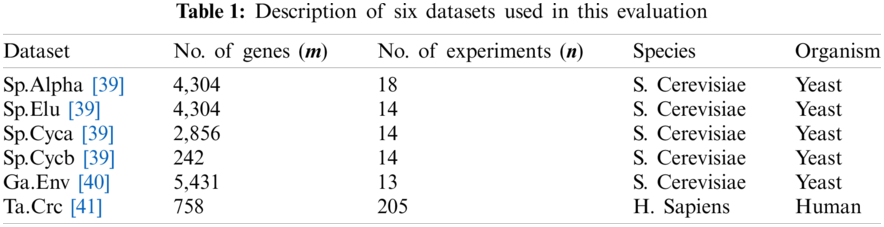
Specific to this empirical study, proposed models are evaluated on six gene expression datasets that are obtained from published microarray experiments. This follows the previous study of [12], which initially introduces the concept of CKNNimpute, i.e., the baseline of OWA-CKNN. Four of these datasets originate from the cell-cycle expression of yeast Saccharomyces Cerevisiae (or S. Cerevisiae) that has been reported in [39]. The first set named Sp.Alpha is represented as an m×n data matrix of m=4,303 genes and n=18 experiments. The second dataset that is referred to as Sp.Elu hereafter is generated from elutriation data and presented as a 4,303×14 matrix. Next, Sp.Cyca is the third set in which time series data for the analysis of cell cycle regulate genes is recorded as a matrix of dimension 2,856×14. The fourth microarray dataset or Sp.Cycb is also drawn from this set of time series, and contains 242 genes and 14 experiments. In addition to these, the fifth dataset is acquired from the study of [40], which investigates response in yeast to environmental changes. This data matrix called Ga.Env contains 5,431 genes and 13 experiments. At last, the sixth dataset or Ta.Crc presents cDNA microarray data [41] relevant to human colorectal cancer (CRC). In particular, the underlying data matrix contains 758 genes and 205 primary CRCs. Details of these six datasets are summarized in Tab. 1. Note that these have been investigated in many studies, including the survey of [6] and comparative reports by [42,43]. Henceforth, these can be considered as the benchmark data collection for the comparison of new and existing imputation methods. In order to make use of these datasets for the problem of missing values, they are modified such that missing values are randomly inserted to make up the proportion of up to r% of the data matrix, where r∈{1,2,3,4,5,10,15,20}. This can be achieved by the salt-and-pepper selection of corresponding positions across the space of m×n.

To gain a thorough comparison of performance, the next five methods are included in experiments in addition to OWA-CKNN and OWA-KNN. The setting of method-specific parameters are also specified.

•   Two basic imputation techniques of zero heuristics and row average, which are referred to as Zero and RA hereafter.

•   Two common neighbor-based models KNNimpute [18] and its weighted variation, WKNN [44]. Algorithmic variables are set in accordance with those reported in published reports.

•   CKNN: cluster-based KNNImpute or called CKNNimpute in the original work of [12]. Note that, as the baseline of OWA-CKNN such that the steps of finding clustering-based nearest neighbor set is identical to that of OWA-CKNN. Furthermore, CKNN is a good representative of many imputation techniques found in the literature as it demonstrates performance superior than others [12] such as SKNNimpute [19], IKNNimpute [20], LLSimpute [45], and BPCAimpute [46].

•   Similar to many previous studies, normalized root mean square error or NRMSE [6] is used to determine a goodness of imputation. It is based on the difference between values estimated by an imputation technique and their true values. Intuitively, the lower such a difference is the better the performance is. Formally, NRMSE is defined by the following. Note that xtruth is the actual value in the original data matrix, xestimate is the corresponding estimated value, var(xtruth) is the variance of the actual values. The lower NRMSE is, the better the value estimated by a computerized method becomes.

NRMSE=mean(xestimate−xtruth)2var(xtruth) (11)

•   Each experiment setting (imputation method, dataset and missing rate) is repeated for 20 trials to generalize the results and comparison.

3.2 Experimental Results

According to Fig. 1 that presents method-specific NRMSE measures as averages across datasets and multiple trials, the two basic alternatives of Zero and RA appear to be the worst among all seven techniques investigated here. The gap of difference between these two with the others is obvious when the missing rate is less than 15%, while KNN is only slightly better than Zero and RA as the rate rises up to 20%. Not only the basic KNN model, performance of other neighbor-based imputation techniques also drops as the magnitude of missing value inclines. Provided that WKNN and OWA-KNN are extensions of KNN, it is only natural to compare their NRMSE scores across the range of missing rates, from 1% to 20%. In particular to this objective, the results illustrated in Fig. 1 suggest that both WKNN and OWA-KNN similarly improve the effectiveness of KNN, whereas OWA-KNN usually provides more accurate estimates than the other for all the missing rates. However, this proposed use of OWA with KNN is still not as good as CKNN, thus confirming the benefit of cluster-based selection of nearest neighbors. This leads to the comparison between OWA-CKNN and its baseline, i.e., CKNN. It is observed that the former performs consistently better than the latter, with the different between their NRMSE scores becomes gradually larger along the increase of missing rate. It is noteworthy that OWA-CKNN is a promising choice as it is able to keep the NRMSE measure below 0.68 even with a large amount of missing values. Apart from this overview, details of dataset-specific results are given next.

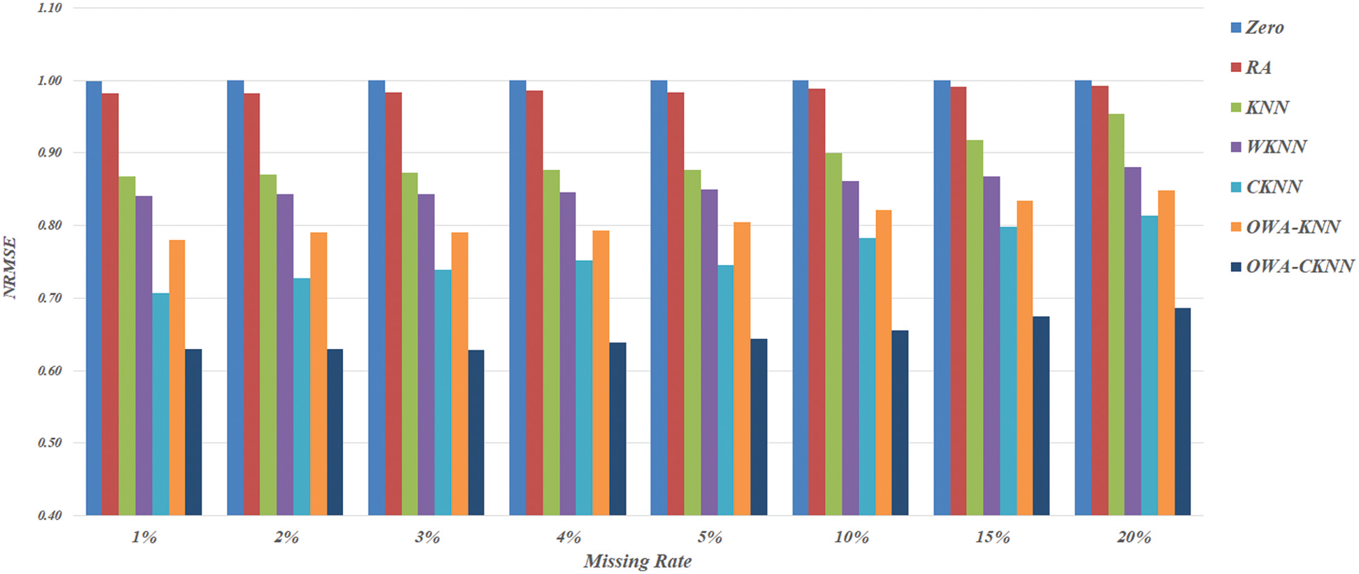
Figure 1: Method-specific NRMSE scores as averages across datasets and multiple trials, categorized by different rates of missing values: 1%, 2%, 3%, 4%, 5%, 10%, 15% and 20%, respectively

Figs. 2–7 provide further results summarized for each of datasets examined in this study. Note that the results of Zero and RA are not included in these figures as they are significantly higher than five neighbor-based counterparts, hence making illustrations rather difficult to understand. With the Sp.Alpha dataset, it is shown that all the four variants of KNN outperform the baseline model, with OWA-CKNN achieving the best NRMSE score for each of missing rates. This trend can be similarly observed with other datasets (based on Figs. 3–7), where NRMSE scores of OWA-CKNN are significantly lower than those of CKNN. It is also interesting to see that OWA-KNN can be more effective than CKNN in datasets like Sp.Elu, Sp.Cyca, Sp.Cycb and Ga.Env. This suggests that the exploitation of OWA operator can provide a reliable estimate even from a set of simple nearest neighbors, i.e., without referring to the cluster-based reference. Specific to Fig. 7 that shows the results with Ta.Crc, OWA-CKNN is able to boost the performance of CKNN, which is originally only comparable to WKNN and slightly better than the KNN baseline.

Figure 2: Method-specific NRMSE scores as averages from multiple trials, on the Sp.Alpha dataset

Figure 3: Method-specific NRMSE scores as averages from multiple trials, on the Sp.Elu dataset

Figure 4: Method-specific NRMSE scores as averages from multiple trials, on the Sp.Cyca dataset

Figure 5: Method-specific NRMSE scores as averages from multiple trials, on the Sp.Cycb dataset

Figure 6: Method-specific NRMSE scores as averages from multiple trials, on the Ga.Env dataset

Figure 7: Method-specific NRMSE scores as averages from multiple trials, on the Ta.Crc dataset

To achieve a more reliable assessment, the number of times (or frequencies) that one technique is ‘significantly better’ and ‘significantly worse’ (of 95% confidence level) than the others are considered. This comparison framework has been successfully used by [37,38] to discover trustworthy conclusions from the results. Let μ(i,j) be the average of NRMSE measures across n runs (n = 20 in this evaluation) for an imputation method i∈CM (CM is a set of seven methods assessed here), on a specific dataset j∈DT (DT is a set of investigated datasets). In other words, μ(i,j) is estimated by the next equation.

μ(i,j)=1n∑t=1nNRMSEt(i,j), (12)

where NRMSEt(i,j) denotes the NRMSE measure obtained from the t-th run of method i, on dataset j. The comparison of average values (or means) to discriminate the effectiveness of examined methods may be misleading, as the difference between means can be statistically insignificant at times. Thus, such an evaluation decision can be more robust using the 95% confidence interval for the mean μ(i,j), which is defined as follows.

[μ(i,j)−1.96S(i,j)n,μ(i,j)+1.96S(i,j)n], (13)

where S(i,j) denotes the standard deviation of the NRMSE measures across n runs for a method i over a dataset j. The statistical significance of the difference between any two techniques i,i′∈CM over any dataset j∈DT is found if there is no intersection between their confidence intervals of μ(i,j) and μ(i′,j). For any dataset j, a method i is significantly better than another method i′ when the following is true.

(μ(i,j)−1.96S(i,j)n)>(μ(i′,j)+1.96S(i′,j)n) (14)

Following that, the number of times that one method i∈CM is significantly better than its competitors across all experimented datasets, i.e., B(i), can be estimated by the following equation.

B(i)=∑∀j∈DT ∑∀i′∈CM, i′≠ibetterj(i,i′), (15)

provided that

betterj(i,i′)={1if(μ(i,j)−1.96S(i,j)n)>(μ(i′,j)+1.96S(i′,j)n)0otherwise………………………………………….. (16)

Similarly, the number of times that one method i∈CM is significantly worse than its competitors, i.e., W(i) can be computed by the next pair of equations.

W(i)=∑∀j∈DT ∑∀i′∈CM, i′≠iworsej(i,i′), (17)

worsej(i,i′)={1if(μ(i,j)−1.96S(i,j)n)<(μ(i′,j)+1.96S(i′,j)n)0otherwise………………………………………….. (18)

Given these definitions, it is useful to evaluate the quality of imputation techniques based on the frequencies of better (B) and worse (W) performance than competitors. Figs. 8 and 9 depict better and worse statistics at low missing rates of 1% and 5%. These lead to a familiar conclusion that OWA-CKNN is the most effective, and another proposed model of OWA-KNN is usually better than both WKNN and KNN. Let use turn to the case of a high missing rate of 20%. The same observation is also obtained from the results shown in Fig. 10. Note that the quality of OWA-CKNN is exceptional in this extreme case as compared to other alternatives. This is implied by the fact that ‘Worse’ frequency of this model is zero. Nonetheless, the goodness of all methods including OWA-CKNN is likely to rapidly decrease as the rate of missing values grows beyond the mark of 20%.

Figure 8: Comparison of better-worse statistics between neighbor-based methods, at 1% missing rate

Figure 9: Comparison of better-worse statistics between neighbor-based methods, at 5% missing rate

Figure 10: Comparison of better-worse statistics between neighbor-based methods, at 20% missing rate

4  Conclusion

This paper presents an organic combination of KNN imputation and argument-dependent OWA operator, which has been missing from the literature, especially for improving quality of gene expression data. Instead of relying on a simple average as the representative of attribute values extracted from a set of nearest neighbors, a weighted aggregation is exploited. Each of these reference values is assigned with a specific weight emphasizing its significant to the underlying summarization. A simple global approach to determine argument-dependent weights is employed in the current work for its simplicity and efficiency. The proposed models of OWA-CKNN and OWA-KNN are assessed against benchmark competitors, over a set of published data and a widely used quality metric of NRMSE. In addition, an additional evaluation framework of significant better and worse is also exploited herein to provide further comparison. Based on the experimental results, both new techniques usually perform better than their baselines, whilst reaching the best performance per setting of dataset and missing rate. Despite this success, it is recommended to make use of other alternatives to resolve the problem of missing values when the rate of missing values grows higher than the level of 20%. Perhaps, a re-run of microarray experiment might be a better choice than analyzing uncertain data. With respect to the current development, several directions of possible future work can be considered. These include the exploitation of consensus clustering [37,47] to provide accurate clusters for the proposed neighbor-based imputation method. In particular, an investigation of generating those using quality-diversity based selection of ensemble members [48] and noise-induced ensemble generation [49] can be truly useful in practice. Besides, possible applications of imputation techniques to fuzzy reasoning [50] and clustering-based data discretization [51] can also be further studied.

Acknowledgement: This research work is partly supported by Pibulsongkram Rajabhat University and Mae Fah Luang University.

Funding Statement: This work is funded by Newton Institutional Links 2020--21 project: 6237188 81, jointly by British Council and National Research Council of Thailand (https://www.britishcouncil.org). The corresponding author is the project PI.

Conflicts of Interest: There is no conflict of interest to report regarding the present study.

References

 1.  A. P. Gasch, M. Huang, S. Metzner, D. Botstein, S. J. Elledge et al., “Genomic expression responses to DNA-damaging agents and the regulatory role of the yeast ATR homolog Mec1p,” Molecular Biology of the Cell 12, vol. 10, pp. 2987–3003, 2001. [Google Scholar]

 2.  X. Wang, A. Li, Z. Jiang and H. Feng, “Missing value estimation for DNA microarray gene expression data by support vector regression imputation and orthogonal coding scheme,” BMC Bioinformatics, vol. 7, no. 1, pp. 32, 2006. [Google Scholar]

 3.  Y. Sun, U. Braga-Neto and E. R. Dougherty, “Impact of missing value imputation on classification for DNA microarray gene expression data: A model-based study,” EURASIP Journal on Bioinformatics and Systems Biology, vol. 2009, no. 1, pp. 504069, 2009. [Google Scholar]

 4.  P. Sethi and S. Alagiriswamy, “Association rule based similarity measures for the clustering of gene expression data,” The Open Medical Informatics Journal, vol. 4, no. 63, pp. 63–67, 2010. [Google Scholar]

 5.  S. Friedland, A. Niknejad and L. Chihara, “A simultaneous reconstruction of missing data in DNA microarrays,” Linear Algebra and its applications, vol. 416, no. 1, pp. 8–28, 2006. [Google Scholar]

 6.  T. Aittokallio, “Dealing with missing values in large-scale studies: Microarray data imputation and beyond,” Briefings in Bioinformatics, vol. 11, no. 2, pp. 253–264, 2010. [Google Scholar]

 7.  C. C. Chiu, S. Y. Chan, C. C. Wang and W. S. Wu, “Missing value imputation for microarray data: A comprehensive comparison study and a web tool,” BMC Systems Biology, vol. 7, no. 6, pp. –S12, 2013. [Google Scholar]

 8.  S. Wu, A. C. Liew, H. Yan and M. Yang, “Cluster analysis of gene expression data based on self- splitting and merging competitive learning,” IEEE Transactions on Information Technology in Biomedicine, vol. 8, no. 1, pp. 5–15, 2004. [Google Scholar]

 9.  A. Brevern, S. Hazout and A. Malpertuy, “Influence of microarrays experiments missing values on the stability of gene groups by hierarchical clustering,” BMC Bioinformatics, vol. 5, no. 1, pp. 114, 2004. [Google Scholar]

10. N. Iam-On, “Improving the consensus clustering of data with missing values using the link-based approach,” Data-Enabled Discovery and Applications, vol. 3, no. 7, pp. 253, 2019. [Google Scholar]

11. J. Maletic and A. Marcus, “Data cleansing: A prelude to knowledge discovery,” in Proc. of Int. Conf. on Data Mining and Knowledge Discovery, Washington DC, USA, pp. 19–32, 2010. [Google Scholar]

12. P. Keerin, W. Kurutach and T. Boongoen, “A cluster-directed framework for neighbour based imputation of missing value in microarray data,” International Journal of Data Mining and Bioinformatics, vol. 15, no. 2, pp. 165–193, 2016. [Google Scholar]

13. D. Napoleon and P. G. Lakshmi, “An efficient k-means clustering algorithm for reducing time complexity using uniform distribution data points,” in Proc. of Int. Conf. on Trends in Information Sciences and Computing, Kochi, Kerala, India, pp. 42–45, 2010. [Google Scholar]

14. M. Pattanodom, N. Iam-On and T. Boongoen, “Clustering data with the presence of missing values by ensemble approach,” in Proc. of Asian Conf. on Defence Technology, Chiang Mai, Thailand, pp. 114–119, 2016. [Google Scholar]

15. R. Wallina and A. Hanssona, “Maximum likelihood estimation of linear SISO models subject to missing output data and missing input data,” International Journal of Control, vol. 87, no. 11, pp. 2354–2364, 2014. [Google Scholar]

16. M. G. Rahman and M. Z. Islam, “Missing value imputation using decision trees and decision forests by splitting and merging records: Two novel techniques,” Knowledge Based Systems, vol. 53, no. 1, pp. 51–65, 2013. [Google Scholar]

17. I. Aydilek and A. Arslan, “A hybrid method for imputation of missing values using optimized fuzzy c-means with support vector regression and a genetic algorithm,” Information Sciences, vol. 233, no. 8, pp. 25–35, 2013. [Google Scholar]

18. O. Troyanskaya, M. Cantor and G. Sherlock, “Missing value estimation methods for DNA microarrays,” Bioinformatics, vol. 17, no. 6, pp. 520–525, 2001. [Google Scholar]

19. K. Y. Kim, B. J. Kim and G. S. Yi, “Reuse of imputed data in microarray analysis increases imputation efficiency,” BMC Bioinformatics, vol. 5, no. 1, pp. 160, 2004. [Google Scholar]

20. L. P. Bras and J. C. Menezes, “Improving cluster-based missing value estimation of DNA microarray data,” Biomolecular Engineering, vol. 24, no. 2, pp. 273–282, 2007. [Google Scholar]

21. J. V. Hulse and T. M. Khoshgoftaar, “Incomplete-case nearest neighbor imputation in software measurement data,” Information Sciences, vol. 259, no. 2, pp. 596–610, 2014. [Google Scholar]

22. S. Zhang, “Nearest neighbor selection for iteratively KNN imputation,” Journal of Systems and Software, vol. 85, no. 11, pp. 2541–2552, 2012. [Google Scholar]

23. R. Pan, T. Yang, J. Cao, K. Lu and Z. Zhang, “Missing data imputation by K nearest neighbours based on grey relational structure and mutual information,” Applied Intelligence, vol. 43, no. 3, pp. 614–632, 2015. [Google Scholar]

24. J. Silva and E. Hruschka, “EACimpute: An evolutionary algorithm for clustering-based imputation,” in Proc. of Int. Conf. on Intelligent Systems Design & Applications, Pisa, Italy, pp. 1400–1406, 2009. [Google Scholar]

25. D. Hong and S. Han, “The general least square deviation OWA operator problem,” Mathematics, vol. 7, no. 4, pp. 326, 2019. [Google Scholar]

26. R. R. Yager, “On ordered weighted averaging aggregation operators in multi-criteria decision making,” IEEE Transactions on Systems, Man and Cybernetics, vol. 18, no. 1, pp. 183–190, 1988. [Google Scholar]

27. A. Kishor, A. K. Singh, A. Sonam and N. Pal, “A new family of OWA operators featuring constant orness,” IEEE Transactions on Fuzzy Systems, vol. 28, no. 9, pp. 2263–2269, 2020. [Google Scholar]

28. D. P. Filev and R. R. Yager, “Analytic properties of maximum entropy OWA operators,” Information Sciences, vol. 85, no. 1–3, pp. 11–27, 1995. [Google Scholar]

29. R. Fuller and P. Majlender, “An analytic approach for obtaining maximal entropy OWA operator weights,” Fuzzy Sets and Systems, vol. 124, no. 1, pp. 53–57, 2001. [Google Scholar]

30. R. R. Yager, “Nonmonotonic OWA operators,” Soft Computing, vol. 3, no. 3, pp. 187–196, 1999. [Google Scholar]

31. M. Lenormand, “Generating OWA weights using truncated distributions,” International Journal of Intelligent Systems, vol. 33, no. 4, pp. 791–801, 2018. [Google Scholar]

32. X. Y. Sha, Z. S. Xu and C. Yin, “Elliptical distribution-based weight determining method for ordered weighted averaging operator,” International Journal of Intelligent Systems, vol. 34, no. 5, pp. 858–877, 2019. [Google Scholar]

33. Z. S. Xu, “Dependent OWA operators,” in Proc. of Int. Conf. on Modeling Decisions for Artificial Intelligence, Tarragona, Spain, pp. 172–178, 2006. [Google Scholar]

34. Z. S. Xu, “Dependent uncertain ordered weighted aggregation operators,” Information Fusion, vol. 9, no. 2, pp. 310–316, 2008. [Google Scholar]

35. T. Boongoen and Q. Shen, “Clus-DOWA: A new dependent OWA operator,” in Proc. of IEEE Int. Conf. on Fuzzy Systems, Hong Kong, China, pp. 1057–1063, 2008. [Google Scholar]

36. W. Li, P. Yi and Y. Guo, “Majority clusters-density ordered weighting averaging: A family of new aggregation operators in group decision making,” International Journal of Intelligent Systems, vol. 31, no. 12, pp. 1166–1180, 2016. [Google Scholar]

37. N. Iam-On, T. Boongoen, S. Garrett and C. Price, “A link-based approach to the cluster ensemble problem,” IEEE Transactions on Pattern Analysis and Machine Intelligence, vol. 33, no. 12, pp. 2396–2409, 2011. [Google Scholar]

38. N. Iam-On, T. Boongoen and S. Garrett, “LCE: A link-based cluster ensemble method for improved gene expression data analysis,” Bioinformatics, vol. 26, no. 12, pp. 1513–1519, 2010. [Google Scholar]

39. P. Spellman, G. Sherlock, M. Zhang, V. Iyer, K. Anders et al., “Comprehensive identification of cell cycle-regulated genes of the yeast Saccharomyces Cerevisiae by microarray hybridization,” Molecular Biology of the Cell, vol. 9, no. 12, pp. 3273–3297, 1998. [Google Scholar]

40. A. Gasch, M. Huang, S. Metzner, D. Botstein, S. Elledge et al., “Genomic expression responses to DNA-damaging agents and the regulatory role of the yeast ATR homolog Mec1p,” Molecular Biology of the Cell, vol. 12, no. 10, pp. 2987–3003, 2001. [Google Scholar]

41. I. Takemasa, H. Higuchi, H. Yamamoto, M. Sekimoto, N. Tomita et al., “Construction of preferential cDNA microarray specialized for human colorectal carcinoma: molecular sketch of colorectal cancer,” Biochemical and Biophysical Research Communications, vol. 285, no. 5, pp. 1244–1249, 2001. [Google Scholar]

42. C. Chiu, S. Chan and W. Wu, “Missing value imputation for microarray data: A comprehensive comparison study and web tool,” BMC System Biology, vol. 7, no. s6, pp. 12, 2013. [Google Scholar]

43. M. Celton, A. Malpertuy, G. Lelandais and A. Brevern, “Comparative analysis of missing value imputation methods to improve clustering and interpretation of microarray experiments,” BMC Genomics, vol. 11, no. 1, pp. 15, 2010. [Google Scholar]

44. G-F. Fan, Y-H. Guo, J-M. Zheng and W-C. Hong, “Application of the weighted K-nearest neighbor algorithm for short-term load forecasting,” Energies, vol. 12, no. 5, pp. 916, 2019. [Google Scholar]

45. H. Kim, G. Golub and H. Park, “Missing value estimation for DNA microarray gene expression data: Local least squares imputation,” Bioinformatics, vol. 20, no. 2, pp. 1–12, 2005. [Google Scholar]

46. S. Oba, M. Sato and I. Takemasa, “A Bayesian missing value estimation method for gene expression profile data,” Bioinformatics, vol. 19, no. 16, pp. 2088–2096, 2003. [Google Scholar]

47. M. Pattanodom, N. Iam-On and T. Boongoen, “Hybrid imputation framework for data clustering using ensemble method,” in Proc. of Asian Conf. on Information Systems, Krabi, Thailand, pp. 86–91, 2016. [Google Scholar]

48. N. Iam-On and T. Boongoen, “Diversity-driven generation of link-based cluster ensemble and application to data classification,” Expert Systems with Applications, vol. 42, no. 21, pp. 8259–8273, 2015. [Google Scholar]

49. P. Panwong, T. Boongoen and N. Iam-On, “Improving consensus clustering with noise-induced ensemble generation,” Expert Systems with Applications, vol. 146, pp. 113–138, 2020. [Google Scholar]

50. X. Fu, T. Boongoen and Q. Shen, “Evidence directed generation of plausible crime scenarios with identity resolution,” Applied Artificial Intelligence, vol. 24, no. 4, pp. 253–276, 2010. [Google Scholar]

51. K. Sriwanna, T. Boongoen and N. Iam-On, “Graph clustering-based discretization of splitting and merging methods,” Human-centric Computing and Information Sciences, vol. 7, no. 1, pp. 1–39, 2017. [Google Scholar]

This work is licensed under a Creative Commons Attribution 4.0 International License, which permits unrestricted use, distribution, and reproduction in any medium, provided the original work is properly cited.