DOI:10.32604/cmc.2022.020263
| Computers, Materials & Continua DOI:10.32604/cmc.2022.020263 | |
| Article |
An Optimal DF Based Method for Transient Stability Analysis
1Department of Electrical Engineering, College of Engineering, Jouf University, Sakaka, 2014, Al-Jouf, Saudi Arabia
2Electrical Engineering Department, College of Engineering, Prince Sattam bin Abdulaziz University, Wadi Addawaser, 11991, Saudi Arabia
3Electrical Engineering Department, Aswan Faculty of Engineering, Aswan University, Aswan, 81542, Egypt
4Department of Electrical Engineering, University of Engineering and Technology Peshawar, Pakistan
*Corresponding Author: Emad M. Ahmed. Email: emamahmoud@ju.edu.sa
Received: 17 May 2021; Accepted: 30 June 2021
Abstract: The effect of energy on the natural environment has become increasingly severe as human consumption of fossil energy has increased. The capacity of the synchronous generators to keep working without losing synchronization when the system is exposed to severe faults such as short circuits is referred to as the power system's transient stability. As the power system's safe and stable operation and mechanism of action become more complicated, higher demands for accurate and rapid power system transient stability analysis are made. Current methods for analyzing transient stability are less accurate because they do not account for misclassification of unstable samples. As a result, this paper proposes a novel approach for analyzing transient stability. The key concept is to use deep forest (DF) and a neighborhood rough reduction approach together. Using the neighborhood rough sets, the original feature space is obtained by creating many optimal feature subsets at various granularity levels. Then, by deploying the DF cascade structure, the mapping connection between the transient stability state and the features is reinforced. The weighted voting technique is used in the learning process to increase the classification accuracy of unstable samples. When contrasted to current methods, simulation results indicate that the proposed approach outperforms them.
Keywords: Transient stability analysis; power system; cascade structure; optimal power flow
The development of grid interconnection and intelligence makes today's power grids increasingly complex and open; while the scale of power grids continues to expand, uncertain risk factors are also increasing [1–5]. This puts forward higher requirements for the safety and stability analysis of the power grid. The transient stability assessment of the power system requires that when a large disturbance occurs, it is required to judge whether the system can maintain a synchronous steady state in time. In the face of complex large power grids, traditional power system transient stability assessment approaches based on physical models have low efficiency [6–13], and it is difficult to satisfy real-time online assessment criteria, and certain simplifications and assumptions that the actual situation causes deviation. Currently, the development of synchronized phasor measurement devices and wide-area measurement systems [14–18] allows researchers to collect massive amounts of power system synchronization data in real time, providing new ideas for researchers to try to solve this problem from a data mining perspective.
The application of various power transmission methods and new energy technologies have made the grid structure and operating conditions more complex, leading to more risks for the safe and stable operation of the power system. Transient stability analysis is an important content of power system safety analysis. At present, the commonly used traditional analytical methods such as time domain simulation, direct method, etc., because the former is computationally intensive and time-consuming, the latter is used in complex systems. It is difficult to construct an energy function that satisfies the conditions and other defects, and cannot meet the real-time requirements of the security and stability assessment of large power grids. Therefore, how to accurately and quickly identify transient stability in the early stage of system failure is a problem that needs to be solved urgently in the online security analysis link, and it is also an important foundation for the realization of the idea of “measurement, identification, and control”.
The transient stability evaluation method based on data mining has attracted more and more scholars’ attention in recent years because it can meet the requirements of real-time online evaluation and has high evaluation accuracy [19–25]. It treats the power system transient stability assessment problem as a two-category pattern recognition problem. By establishing a set of transient feature sets that are strongly related to the transient stable state and collecting a large amount of sample data, the classification model is used to perform offline learning of the nonlinear mapping relationship between the transient feature set and the transient stable state. Furthermore, the trained classification model is used to conduct online evaluation of the newly received power grid sampling data to meet the requirements of real-time transient stability evaluation [26–29]. Compared with the traditional physical model-driven transient stability evaluation method, the data-mining-based transient stability evaluation method is data-driven and has higher evaluation accuracy while satisfying the rapidity of evaluation [30–35].
The current research on transient stability assessment methods based on data mining mainly includes two aspects: feature selection and classifier construction. In the study of feature selection, there have been methods such as principal component analysis [36,37], cultural algorithm [38], support vector machine [39] for transient feature extraction, and good results have been achieved. In terms of classifier construction, the current transient stability assessment models mainly include support vector machines [33,40–44], decision trees [45–47] and neural networks [36,48,49]. Among them, literature [40,41] propose power grid transient stability assessment methods based on integrated multiple support vector machines from the perspective of model parameters and input feature space. Reference [33] improves on traditional support vector machines, and proposes a regularized projection twin support vector machine transient stability assessment method. Literature [45,46] designs prediction models based on decision trees. However, the methods mentioned above are all shallow models, and the accuracy of the evaluation still needs to be further improved. In addition, shallow models often have problems such as poor generalization ability and low training efficiency when processing large-scale grid data [50]. In contrast, transient stability assessment methods based on deep learning models have more advantages. On the one hand, through the multi-layer serial deep architecture, abstract characterization learning of features can be performed to strengthen the nonlinear mapping relationship between feature quantities and label attributes. On the other hand, compared with the shallow model, the deep learning method has stronger learning ability and generalization ability, and the evaluation accuracy is higher. However, deep learning models usually need to be built on the basis of a large number of sample data. In the case of a small number of samples, due to insufficient fitting accuracy of the data distribution, the evaluation accuracy is usually low. In addition, in order to make an unbiased estimation of the distribution of training samples, the existing deep learning methods represented by deep confidence networks [50–53] often assume that the distribution of transiently stable samples and transiently unstable samples is balanced, and lacks Pay attention to transient instability samples. In the actual grid operation, the grid maintains a transient stable state in most cases, and transient instability is very rare. Therefore, the data volume of transiently stable samples and transient instability samples is often obviously unbalanced. relationship. In order to improve the accuracy of evaluation when learning and training traditional classification models, they tend to place more emphasis on transiently stable samples that account for the majority of samples, resulting in lower classification accuracy for transiently unstable samples. In practice, if a transient instability sample is misjudged as a transient stable sample, it will affect the system dispatchers to take protective measures in time, posing a major threat to the security of the power grid. Therefore, on the basis of ensuring the overall evaluation performance, more attention should be paid to the accuracy of the evaluation of transient instability samples.
In light of the aforementioned issues, this research provides a power system transient stability assessment approach that combines neighborhood and deep forest rough reduction. The forest created by decision tree integration is further integrated, and the original transient features’ representation learning is accomplished using the cascade approach to abstractly produce a high-dimensional feature space that is better suited to classification learning. To further boost the deep forest's characterization learning capacity, we used neighborhood rough reduction to locate numerous sets of various optimal feature subsets at varying degrees of granularity to re-characterize the original feature space. The classification algorithm now pays greater attention to transient instability samples thanks to the addition of a weighted voting mechanism. The experimental findings suggest that the proposed strategy may successfully minimize the misclassification rate of transient instability samples while also improving evaluation accuracy. In comparison to classic deep learning approaches, the suggested technique produces superior assessment results even when the sample size is small, is less impacted by irrelevant features and sample set imbalance, and has some robustness and application.
The core of the transient stability assessment method based on data mining is to design a classification model to learn and fit the complex non-linear mapping relationship between the transient characteristic quantity of the power grid and the transient stable state (category). The transient feature set with highly correlated state is the foundation and key of this kind of method. There are currently two ways to construct the initial transient feature set of the power grid. The first type directly constructs the initial transient feature set based on the power flow of the system before and after the fault, such as the voltage amplitude, phase, active and reactive power distribution of each bus in the system. This method directly learns the classifier based on the original data at the bottom of the power grid, and does not rely on expert experience for feature selection [48], but the scale of the selected transient feature quantity fluctuates greatly with the change of the system scale. In actual large systems, too many input features will not only cause serious computational burden, reduce the accuracy of the classification learning algorithm, but also prone to “dimensionality disaster” phenomenon [38]. The second is to construct an initial feature set based on the combined variables of the system parameters before and after the fault. The transient stable state can be fully characterized by considering the selection of “combined characteristic quantities” of a group of systems under different time and space factors. This method requires certain expert experience knowledge, but the advantage is that the selected feature set is fixed and does not change with the change of the system object, and it is more general. At the same time, considering the completeness in time and space, it can better reflect the impact of changes in the operating environment on the transient stability characteristics of the system. This article chooses the second method to construct the initial transient feature set.
When using the “combined feature quantity” method to construct the initial transient feature set, three aspects: the systematic principle, the mainstream principle and the real-time principle are usually considered [38,49,54], that is, the selected feature quantities must meet: 1) The scale of the selected feature quantity does not change with system changes, and should be the combined index of the state variables of each component in the system; 2) There is a high correlation between the selected feature quantity and the transient stable state; 3) The chosen feature quantity must be completed in a timely manner, and it must represent the state of the system before and after the fault occurs in order to fully comprehend the fault's effect on the system. According to the above three principles, on the basis of a large number of simulation experiments, and based on the study and summary of the existing literature [43–45,49,50,54–56], the 32-dimensional transient characteristic quantities were determined.
It can be seen that the transient characteristic quantities constructed in this paper are not affected by the scale of the system, and are all combined indicators of the state variables of the components in the system. In terms of time, it covers the three different phases of the system state at the time of steady state (features 1 and 2), the time of fault occurrence (features 3∼11) and the time of fault clearing (features 12∼32), which can fully reflect the fault brought to the system impact. The selection of characteristic quantities is mainly based on the combination of system physical quantities reflecting the rotor state and system operation level. Among them, the characteristics 6, 7, 17∼19, 29 are related to the rotor angle, reflecting the synchronous operation state of the generator; the characteristics 5, 8∼15, 20∼27, 30, 31 are related to the rotor speed and acceleration, reflecting the disturbance The influence of rotor movement; characteristics 1∼4, 16, 28, 32 are related to the operating level of the system, reflecting the influence of the fault on the power balance of the system. Therefore, the established transient feature set can well reveal the impact of fault impact on the system stability trend.
4 Basic Principles of the Model
From the point of view of data mining, power system transient stability assessment is essentially a process of learning and classifying the corresponding data set. In order to facilitate the analysis, this article describes the classification task as a decision system
4.1 Rough Neighborhood Reduction
Since the construction of transient features relies on expert experience, after the initial transient feature set is constructed, it can usually be further compressed or reduced to extract key features and reduce the redundancy of the feature set [39,42,56]. For this reason, this paper introduces the method of neighborhood rough set [57] to further reduce the initial transient feature set.
For a classification task of transient stability assessment
In the formula,
Further, the entire sample set is divided into a stable sample set 1d and an unstable sample set
where
It can be seen from Eq. (2) that if a sample is in the positive domain, all samples with similar feature values have the same label category. This shows that the sample can be accurately classified under the feature set B. The more samples in the positive domain, the better the separability of feature set B and the stronger the classification ability, which is more conducive to the learning of classification algorithms. Similarly, call
For the classification task of transient stability assessment
For each feature
If
By setting different neighborhood thresholds δ, the neighborhood particle size of the sample can be controlled, and the reduction results at different granularity levels can be obtained.
A decision tree is a classification model with a tree structure, which starts from the root node and performs feature selection and sample partitioning at each child node to obtain different node rules. Each child node corresponds to a feature, and each node rule represents a way to divide the sample under the selected feature. According to the obtained node rules, different samples are assigned to each child node in turn. The above process is recursive, and the sample is continuously divided until it reaches the leaf node. Each leaf node represents a category label of the sample. For decision trees, the feature selection at each node and the way of sample division are very important. The commonly used measurement methods for feature selection of decision tree nodes usually include information gain ratio and Gini index. For a classification task of transient stability assessment
If the sample set U is divided into two parts
The information gain ratio of feature c to data set U is defined as
For the sample set U, the Gini index is defined as
The Gini index of feature c on the data set U is defined as
Through the integration of multiple decision trees, a decision tree forest can be further formed. The decision tree forest is an ensemble learning model, which votes in a way that the minority obeys the majority and gives the final decision result. Because it comprehensively considers the prediction results of multiple models, it has high evaluation accuracy and strong robustness. According to the input space composition of the sub-classifier and the feature selection method, the decision tree forest can be further divided into random forests [58], completely random tree forests [59] and extreme random trees [60]. Specifically, for a decision-making system containing n input features, the random forest randomly selects m (m < n) sub-features as the input feature set of each tree, and in the random subset according to the information gain ratio or Gini index to find the best feature and division point on each node. This paper adopts the empirical value
Deep forest [58,61] is an integrated model based on decision tree forest under deep architecture. It strengthens the diversified learning ability of the model by further integrating multiple different decision tree forests and realize multi-layer representation learning in deep learning architecture. The deep forest mainly includes two parts: the cascade structure and the enhancement and characterization of input features.
5.1 Cascade Forest Structure and Voting Weighting Mechanism
The deep forest is composed of multiple learning layers in series, where each learning layer is integrated by several decision tree forests. The output probability vector of each layer to the sample label together with the original input features reconstitutes the input features of the next learning layer, and the cascade structure is shown in Fig. 1.
The decision tree forest is composed of several decision trees, and each decision tree will output the corresponding transient stability assessment results. For each decision tree forest in the learning layer, by calculating the proportion distribution of trees with stable evaluation results and trees with unstable evaluation results in the forest, a two-dimensional class distribution vector is finally generated, indicating that the samples are located in different transient states probability in the state. If each level contains M decision tree forests, each layer will output M 2-dimensional probability vectors about the class distribution, which are connected in series to form a 2 × M-dimensional enhanced feature. These 2 × M-dimensional enhanced features will be connected together with the original 32-dimensional input features to form a new feature vector of is used as the input feature of the next learning layer. Through the step-by-step abstract reinforcement of the feature vector, high-order features that are more conducive to classification learning can be extracted, and the multi-layer representation learning effect in the deep learning framework can be achieved. In order to ensure diversification of learning, in each level of learning, this paper selects random forests based on information gain ratio and Gini index (respectively marked as RFI and RFG), and completely random tree forests based on information gain ratio and Gini index (respectively recorded respectively). There are five different types of forests (CRFI and CRFG) and extreme random trees (denoted as ERF).
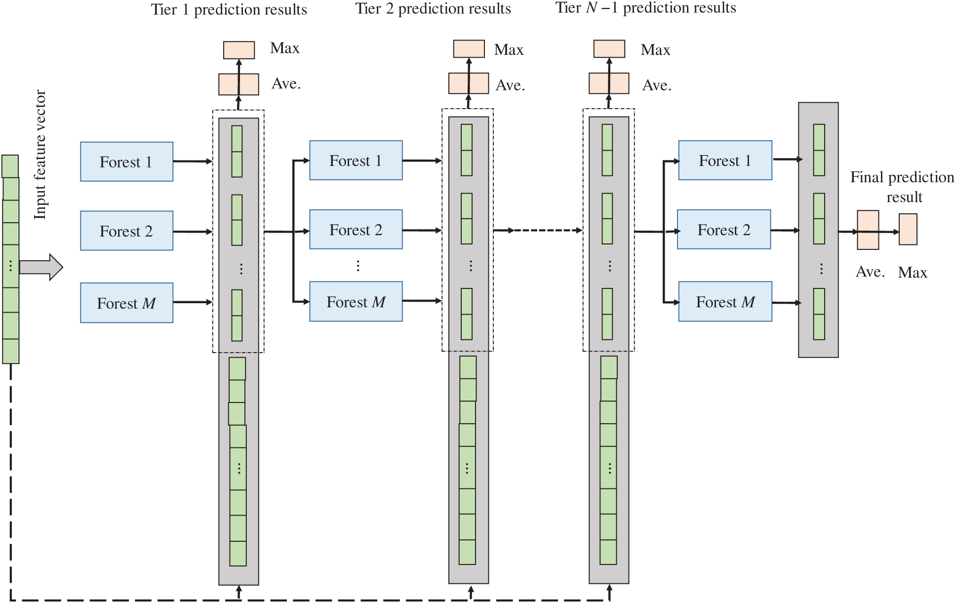
Figure 1: DF architecture
In the power system transient stability assessment problem, the transient instability samples are often small, and there is an obvious imbalance in the number of transient stability samples, so the classifier tends to learn in the direction that is conducive to the classification of transient stability samples. However, the cost of misjudging transient instability samples is higher, so in practice, more attention should be paid to improving the assessment accuracy of transient instability samples. For this reason, when the class distribution vector is generated at each level, the weighted voting mechanism shown in Fig. 2 is introduced to strengthen the importance of transient instability samples in the learning process.
For a classification task of transient stability assessment
Eqs. (7) and (8) respectively represent the conditional probability of transient stability and transient instability when the eigenvalues are input for a given sample. It adaptively weights the class vectors according to the degree of imbalance between the two types of samples, and gives higher weight to the transient instability samples. The more serious the imbalance of the sample, the higher the weight assigned to the unstable sample. Therefore, in the learning process, the emphasis on transient instability samples can be better strengthened, and the misjudgment of transient instability samples can be reduced.
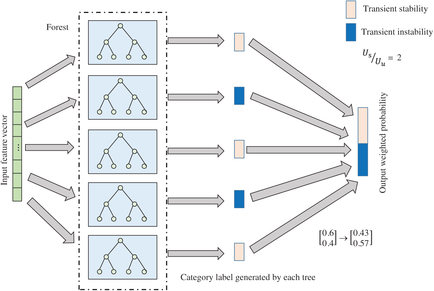
Figure 2: Paradigm for weighted voting
In the training process of the deep forest, each additional level will be aligned with each level of the forest on the verification set for verification and evaluation. For each input of a prediction sample, the probability vectors generated by all forests are averaged at each level of learning, and the category with the largest probability output will be used as the prediction label of the sample. If the classification performance does not increase, stop training.
5.2 Input Features to Enhance Re-Characterization
Compared with the shallow learning model, the advantage of the deep learning method lies in its powerful ability to deal with feature relationships. By re-characterizing the original feature space, the relationship between the feature quantity and the label attribute can be strengthened. Non-linear mapping relationship, thereby further strengthening the representation learning ability of deep forest [61]. This paper uses neighborhood rough reduction to find multiple sets of different optimal feature subsets at different granularity levels to re-characterize the original feature space, as shown in Fig. 3.
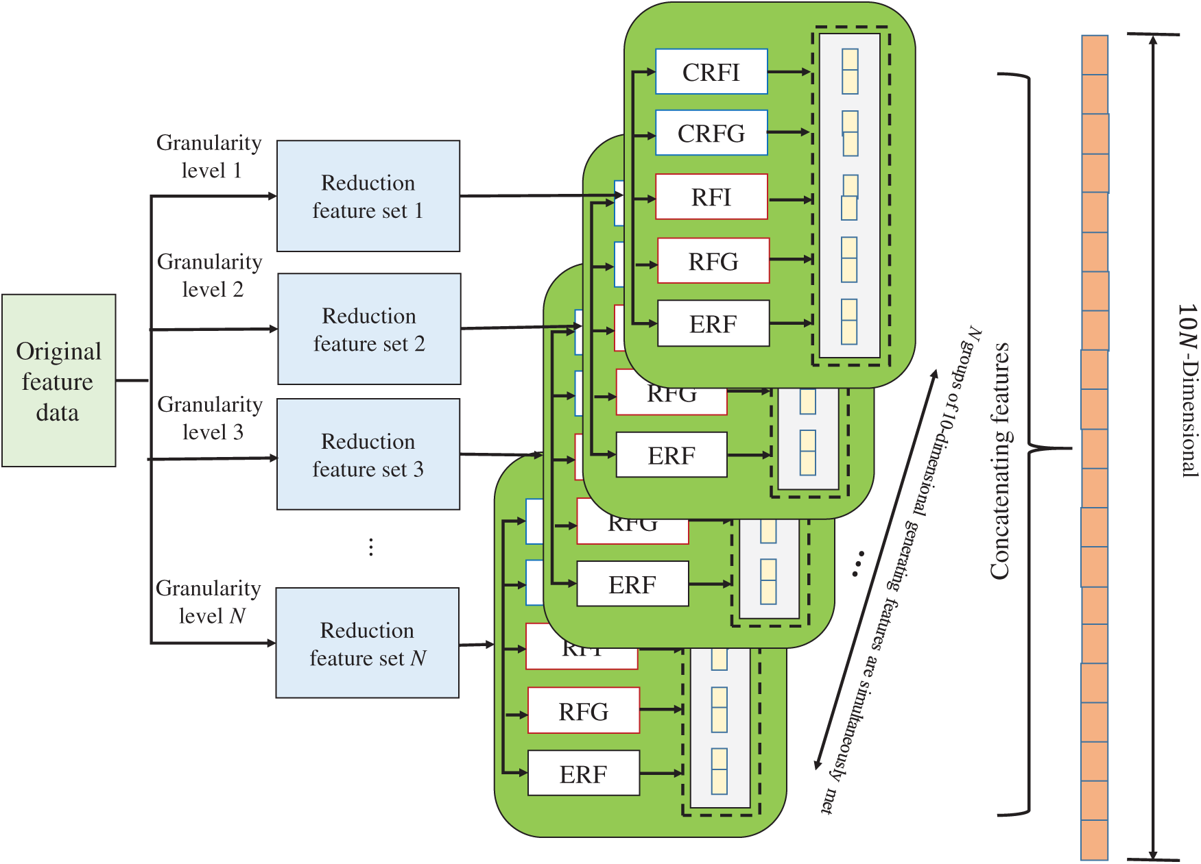
Figure 3: Architecture for re-characterization
In Fig. 3, by setting different neighborhood thresholds for the rough reduction of the neighborhood, the original feature space is reduced to several different feature subspaces. Use five forests of RFI, RFG, CRFI, CRF and ERF to train the samples in each feature subspace. Each forest will generate a 2-dimensional probability vector about the class distribution, so the sample will generate a 10-dimensional probability vector in each feature subspace. By concatenating the probability vectors generated under the N feature subspaces, the original 32-dimensional initial feature vector will be re-characterized as a 10 × N-dimensional high-order feature. The enhanced re-characterization of the input features provides more sufficient information than the original feature space, and the greater the difference in the selected feature subspaces, the stronger the representation ability and the better the learning effect.
Fig. 4 shows the overall evaluation model integrating rough reduction of neighborhood and deep forest. Use neighborhood rough reduction to find several different feature subspaces at different granularity levels, and re-characterize the original feature vector under these feature subspaces. Each level of the deep forest learning layer is composed of five different types of decision tree forests, and each layer will output a 10-dimensional class vector, which will be used as an enhanced feature and a re-representation feature in series to form the next level of learning layer Input characteristics. Assuming that the dimension of the re-characterization feature is 60, the input of each level is a high-order abstract feature of 70 (=60 + 10) dimensions. The final model will take the average of the 2-dimensional class vectors generated by the last level of the five types of forests, and output the label with the highest probability as the model prediction result.
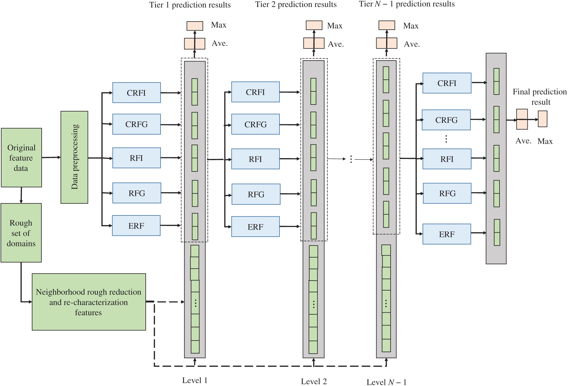
Figure 4: Overall evaluation framework
The transient stability assessment model framework proposed by the transient stability assessment process combining rough reduction of neighborhood and deep forest is shown in Fig. 5. It mainly includes two parts: offline model training and online transient stability evaluation. The feature data is sampled offline through time-domain simulation, the feature subspace is determined by the rough reduction of the neighborhood and the original input features are re-characterized, and then deep forest model training is performed on this basis. Whenever the online feature data of the power grid is received, it is re-characterized in the feature subspace obtained from the rough reduction of the offline neighborhood, and then sent to the trained deep forest model for simultaneous evaluation, giving the power grid transient stability The prediction result of the state, for the grid dispatcher to make further decisions policy to provide support.
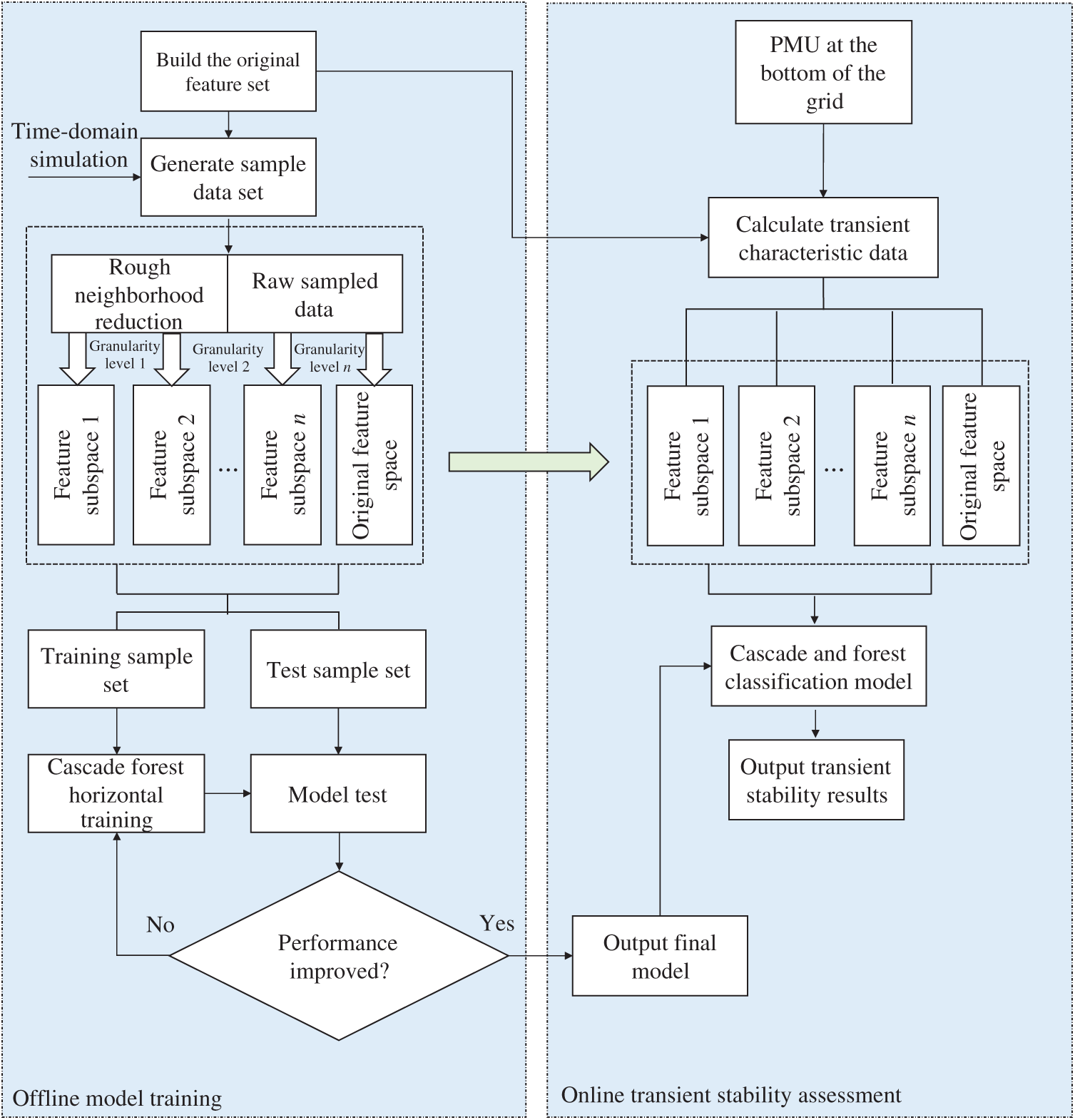
Figure 5: Proposed model for transient stability analysis
In order to verify the effectiveness of the evaluation model proposed in this paper, time-domain simulation was performed on the IEEE 10-machine 39-node system [62], and data collection was performed according to the characteristics in Tab. 1. Two operating environments of standard system topology and N − 1 failure are considered in the simulation. In the N − 1 fault environment, it is assumed that any transmission line or transformer in the system fails due to a fault. With 5% as the step length, set a total of 10 different load levels from 80% to 125%, and at the same time change the generator output accordingly. Twenty fault locations are randomly selected under each operating environment, the fault type is set to three-phase short circuit, assuming that the fault occurs in 0.1 s, and the fault is cleared at 0.2, 0.25, 0.3, and 0.35 s respectively. After the fault is cleared, the lines overlap and the system topology remains unchanged. The simulation duration is set to 5 s. At the end of the simulation, whether the power angle difference of any two generators in the system exceeds 180° is used to judge the transient stable state of the system. If it exceeds 180°, the transient instability of the system is judged, and the corresponding category label is recorded as 0. Otherwise, the system is judged to be stable and the category label is denoted as 1.
The above simulations are all realized in MATLAB/Simulink. The simulation have total 8000 data samples, which 5104 is specified for training set and 2896 is for test set. The K-Means method is deployed to discretize the continuous input value. After completing the sample sampling, the Min-Max standardization method is used to normalize all the sample data to eliminate the influence of the difference in attribute dimension on the learning process.
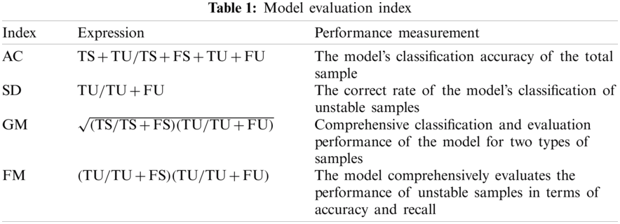
Given that the power system transient stability assessment problem has the characteristics of sample imbalance and misclassification cost imbalance, in order to describe the performance of the model more comprehensively, the classification accuracy (AC) and safety (SD) shown in Tab. 1 are selected in the experiment. G-means indicator (GM) and F-measures indicator (FM) are for performance evaluation. In the table, TS, FS, TU, FU represent the number of stable samples correctly classified, the number of stable samples incorrectly classified, the number of unstable samples correctly classified, and the number of unstable samples incorrectly classified. Among them, the degree of safety reflects the accuracy of the model's classification of transient instability samples. The greater the degree of safety, the lower the rate of misclassification of transient instability samples and the higher the relative safety of the system. The G-means indicator comprehensively considers the evaluation accuracy of transient stable samples and transient instability samples. The larger the G-means value, the more balanced the model's learning of different types of samples, and the better the evaluation performance. The F-measures indicator comprehensively considers the evaluation accuracy and recall rate of unstable samples. The F-measures value will only increase when the accuracy of classifying unstable samples is improved while maintaining a low level of sacrifice for stable samples. In order to avoid the contingency of the experimental results, this paper uses a ten-fold cross-validation method to calculate the performance indicators of the above models in the experiment.
The model parameters mentioned in this paper mainly fall into two categories, including the setting of the neighborhood threshold in the rough reduction stage of the neighborhood and the number of trees contained in the decision tree forest in the model. In the rough reduction stage of the neighborhood, first, according to the recommended neighborhood threshold range [0.1, 0.3] in [57], set the corresponding neighborhood threshold with a step size of 0.02 to perform the reduction operation, and select the largest group of reduction results are used as the final feature subset. Specifically, each selected feature subset should have at least 30% different features to ensure the diversity of learning. In addition, in order to ensure that the re-characterized features have better classification performance, they are usually mapped to a higher-dimensional space for high-level abstraction. At the same time, considering that the memory overhead of the converted data should not be too large, it is usually re-characterized. The size of the feature set can be taken as 2∼4 times of the original feature set. Correspondingly, a different number of feature subsets can be obtained by the neighborhood rough reduction method. In this paper, 6 groups of feature subsets are selected, and the results are shown in Tab. 2.
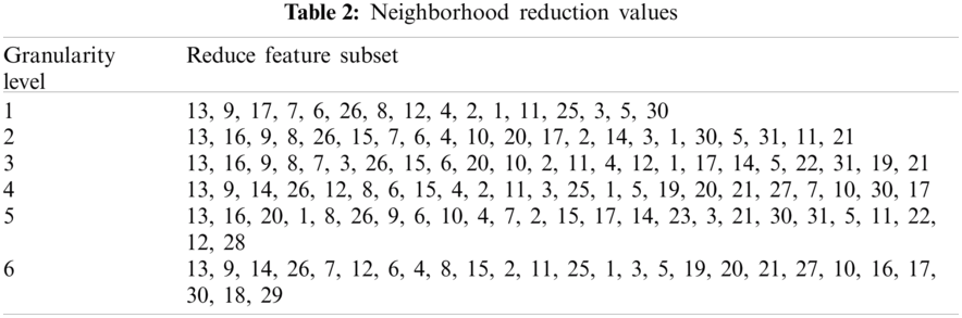
The order of the features in Tab. 2 is given in the order selected in the neighborhood rough reduction algorithm. The final selected feature subset has a total of 6 groups. By enhancing the original input features under the corresponding feature subspace, a 60-dimensional re-characterization feature can be obtained, which will be further concatenated with the 10-dimensional class vector of each level of learning layer, they form 70-dimensional high-level abstract features and participate in learning as the input features of the next level.
Further study the influence of the number of trees contained in the decision tree forest on the performance of the model. With 5 as the step size, the number of trees in the decision tree forest is set to change from 5 to 25. Ten-fold cross-validation was used to evaluate the performance of the model under different parameters. The results are shown in Tab. 3.
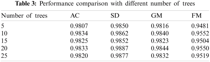
It can be seen from Tab. 3 that when each decision tree forest contains more than 10 decision trees, the performance of the model no longer improves significantly, and it begins to stabilize. In order to reduce the computational load of the model and avoid unnecessary waste of storage space, in the following experiments, this paper assumes that each forest in the model contains 10 decision trees.
6.3 Performance Comparison of Different Models
In order to verify the performance of the model, the commonly used power system transient stability assessment classifiers are selected for comparative analysis. The selected classifier models include C4.5 decision tree, classification regression tree (CART), naive Bayes (NB), support vector machine (SVM), and artificial neural network (ANN). Among them, the ANN uses a three-layer hidden layer structure, and the training algorithm uses a momentum gradient descent algorithm; SVM uses the default parameter settings of the MATLAB toolbox (linear kernel, sequence minimum optimization algorithm). For convenience, the algorithm in this paper is abbreviated as NRRDF in the following. The results are shown in Tab. 4.
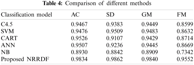
It can be seen from Tab. 4 that compared with other methods, the proposed method has the best performance on the four evaluation indicators. It not only has higher overall evaluation accuracy, but also can improve the performance of transient instability samples. Pay attention to effectively reduce the misjudgment of transient instability samples. Taking ANN as an example, the overall classification accuracy of the proposed model is increased by 3.27%, while the classification accuracy for transient instability samples is increased by 6.26%. This is caused by the learning limitations of the shallow model itself. On the one hand, the shallow model cannot perform efficient characterization learning for feature input, and it is difficult to fully extract useful information in the feature, so the generalization learning ability for many complex nonlinear mapping problems is limited. On the other hand, the existing methods all assume that samples of different categories are evenly distributed in the learning process, and lack of attention to sample imbalance. In contrast, the proposed model can effectively perform high-level abstract transformation of feature information through the enhanced re-characterization of the original feature input and the multi-level serial feature learning structure under the in-depth framework, and dig more hidden in rich information in the data improves the learning ability of the model. In addition, since the class vector is adaptively weighted according to the sample imbalance in the learning process, the transient instability samples are given higher weights, so the model can effectively increase the importance of transient instability samples and reduce false judgment rate.
In order to further reflect the adaptability of the model to the characteristic data under the untrained grid topology, all 800 sets of data collected under a certain grid topology are randomly selected as test data, and the remaining 7200 sets of data collected under other topologies are used as training data to test the performance of the above models, and the results are shown in Tab. 5.
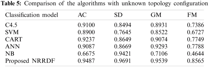
It can be seen from Tab. 5 that without training, the classification performance of each model for characteristic data under the new power grid topology has decreased. Among them, the NB drops the most, because it is an algorithm based on sample probability, which will have a greater impact on performance when the probability distribution of the sample is not fully learned. The performance of C4.5, CART, SVM, ANN, etc. is relatively stable, but the performance of the safety index of the characteristic data under the new topology is poor, which means that it has a higher rate of misclassification of new transient instability samples. In contrast, the proposed NRRDF is not only relatively stable, but also has the best performance on the four indicators, which shows that it has good adaptability to the feature data under the untrained grid topology. The model in this case is more robust.
6.4 Model Performance Under Different Sample Sizes
This section further studies the performance of the model under different sample sizes. Since one of the characteristics of deep learning is the ability to efficiently learn big data, this section selects the most representative deep belief network (DBN) in deep learning for performance comparison. From the original 8000 sets of sample data, using 1000 as the step size, randomly select 1000 to 8000 sets of sample data; under different sample sizes, ten-fold cross-validation is used to evaluate the performance of the proposed model and DBN. The DBN has selected a 3-layer network structure of {10-15-20}, which has been passed many times according to the empirical method. The experiment selects the network structure parameters under the optimal results. The experimental results are shown in Fig. 6.
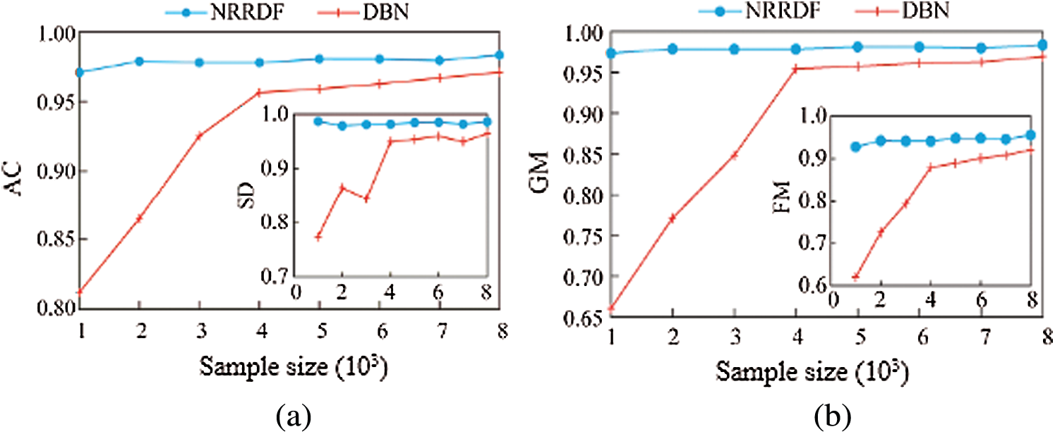
Figure 6: Comparison of the proposed and existing algorithm with increasing number of samples. (a) A, (b) GM
It can be seen from Fig. 6 that when the number of samples is small, the performance indicators of DBN have a large gap compared with NRRDF; as the number of samples increases, the performance indicators of DBN gradually improve and the smaller the number of samples, the more obvious the performance improvement effect brought by increasing the samples. When the number of samples reaches 4000, the performance indicators of DBN begin to become saturated and show a slow increase trend. In contrast, the proposed model is less affected by the number of samples, and has better performance under different sample sizes. When the sample size is small, the proposed model has obvious advantages. Although the gap between the two gradually becomes smaller as the number of samples increases, the proposed NRRDF performance is ultimately better than DBN in all four evaluation indicators. This is because unlike DBN, the proposed NRRDF does not rely on big data to estimate the sample distribution unbiased. In addition, the model depth of DBN is usually a fixed structure, and the proposed model depth can be adaptively determined by evaluating the training process layer by layer during the learning process. Therefore, the proposed model has good performance under different sample sizes and has strong robustness.
6.5 The Impact of Irrelevant Features on Model Performance
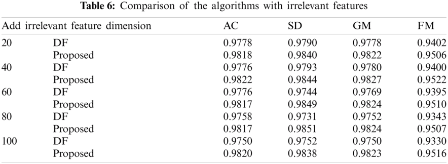
Since the establishment of the transient feature set relies on expert experience, it may be affected by certain human subjective factors. This section studies the influence of irrelevant features on the model. Irrelevant features are generated by random variables that follow a standard normal distribution. Take 20 as the step size to the original data set, add 20–100 dimensional irrelevant features, and use ten-fold cross-validation to calculate the performance index changes of the model when adding different dimensional irrelevant features. In order to show the performance of the proposed model more intuitively, the corresponding evaluation results of the original deep forest model (denoted as DF) that do not adopt the neighborhood rough reduction method to strengthen and re-characterize the input features are given. The results are shown in Tab. 6. It can be seen from Tab. 6 that the performance of the model proposed in this paper is relatively stable after adding different numbers of irrelevant features, and is basically not affected by irrelevant features. The evaluation effect of DF gradually decreases as the number of irrelevant features increases. This is because in the proposed model, the original input features are enhanced and re-characterized by the neighborhood rough reduction method, and the neighborhood rough reduction can effectively mine the key feature set, and the result will not be affected by the number of irrelevant features. Therefore, despite the addition of high-dimensional irrelevant features, the re-characterized features will not be affected. This shows that the method proposed in this paper has strong robustness, and can still guarantee high evaluation performance when a large number of irrelevant features are added.
6.6 Performance Evaluation Under Different Sample Imbalance Ratios
In the actual power grid operation process, because the transient instability of the power grid is very rare, the transient instability samples in the actual power grid data tend to be relatively small. In order to evaluate the performance of the proposed model under different sample imbalance ratios, this paper first randomly selects transient stable samples equal to the transient instability samples from the total sample, so that the proportion of transient instability samples reaches 50%. Then on this basis, some samples were randomly deleted from the transient instability samples, so that the proportion of transient instability samples in the total samples was reduced to 40%, 30%, 20% and 10%. The performance evaluation of the model is carried out under different imbalance degrees, and the G-means and F-measures indicators obtained from the evaluation of each model are shown in Fig. 7.
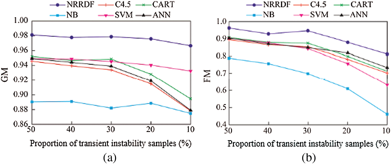
Figure 7: Performance evaluation of the algorithms under transient instability samples (a) GM (b) FM
It can be seen from Fig. 7 that when the number of transiently stable samples and transiently unstable samples are balanced, the classification performance of each model is the best. As the proportion of transient instability samples decreased, the imbalance between the two types of samples gradually increased, and the classification performance of each model began to decline. From the perspective of G-means indicators, the CART, C4.5 and ANN are greatly affected by the decrease in the proportion of transient instability samples, while the model performance of NRRDF, SVM and NB is relatively stable under different sample imbalances. However, the evaluation performance of SVM and NB is poor. In contrast, the proposed model not only has the best performance under the G-means index, but is also relatively stable. From the F-measures index, the performance of various models generally decreases as the proportion of transient instability samples decreases. This is because as the imbalance between samples gradually intensifies, each model gradually biases towards more stable samples in the learning process, and the misclassification rate for transient instability samples tends to be higher. The proposed method adaptively adjusts the weight of transient instability samples according to the degree of imbalance between samples, which can strengthen the emphasis on transient instability samples to a certain extent, and reduce the misclassification of instability samples. Each sample has better classification performance under unbalanced ratio.
Fig. 8 compared the accuracy of the proposed and DBN algorithms. As can be seen from Fig. 8, as the number of iterations increases, the accuracy of both algorithms improves. However, the proposed algorithm gives better accuracy about 99.7% as compared with DBN algorithm which makes it suitable for deploying in power systems transient stability analysis.
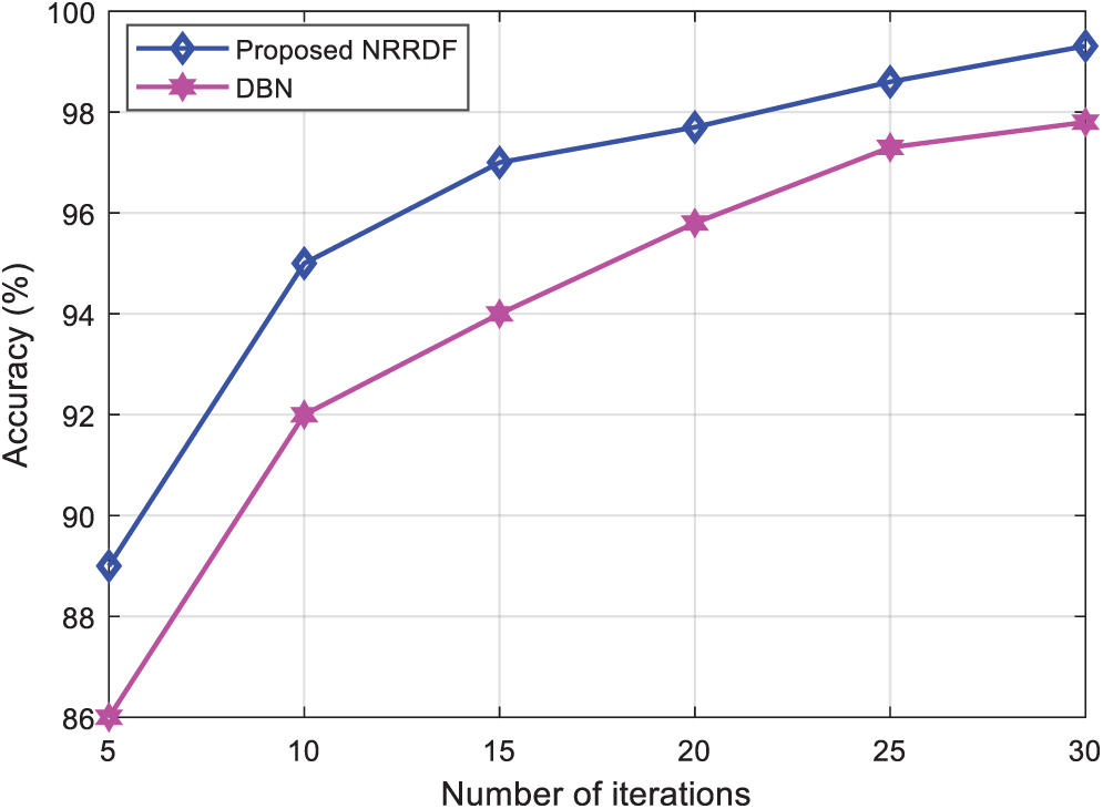
Figure 8: Accuracy comparison
Aiming at the problems of current power system transient stability assessment methods that have limited learning accuracy of shallow models and insufficient attention to transient instability samples, a transient stability assessment method combining rough neighborhood reduction and deep forest is proposed. A comparative experiment analysis of the proposed model is carried out on an IEEE 10-machine 39-node system. Experimental results show that: 1) Compared with the commonly used shallow learning models, the proposed model can effectively improve the classification performance. The introduction of the weighted voting mechanism can effectively improve the model's attention to transient instability samples during the learning process, reduce the misjudgment of transient instability samples, and improve the imbalance of different samples. Both have good performance; 2) Compared with traditional deep learning methods represented by deep belief networks, the proposed method has fewer hyper-parameters. The multi-level sequential structure can not only realize the multi-layer representation learning of the input features, but also can adaptively determine the depth of the model through the layer-by-layer evaluation of the training process during the learning process, so that the proposed model has different scales of data and good performance; 3) Enhancing and re-characterizing the original input features through the neighborhood rough reduction method can not only provide more sufficient information than the original feature space, but also enable the model to maintain high classification performance even when a large number of irrelevant features are added. Therefore, the model robustness is stronger.
In view of some current problems, this paper studies the power system transient stability assessment problem under the deep forest framework. In practice, the loss of transient characteristic data may be caused due to problems such as the loss of measurement devices and communication delay. Therefore, the feasibility analysis of the proposed model under circumstances such as missing data will be perfected in the future.
Funding Statement: The authors extend their appreciation to the Deanship of Scientific Research at Jouf University for funding this work through research Grant No. (DSR-2021-02-0113).
Conflicts of Interest: The authors declare that they have no conflicts of interest to report regarding the present study.
1. M. Rawa, S. Alkhalaf, L. M. Popa, R. Aboelsaud, T. Khurhaid et al., “An efficient scheme for determining the power loss in wind-pv based on machine learning,” IEEE Access, vol. 9, pp. 9481–9492, 2020. [Google Scholar]
2. Q. Su, H. U. Khan, I. Khan, B. J. Choi, F. Wu et al., “An optimized algorithm for optimal power flow based on deep learning,” Energy Reports, vol. 7, pp. 2213–2124, 2021. [Google Scholar]
3. S. Impram, S. V. Nese and B. Oral, “Challenges of renewable energy penetration on power system flexibility: A survey,” Energy Strategy Reviews, vol. 31, pp. 1–12, 2020. [Google Scholar]
4. J. Liu, H. Sun, Y. Li, W. Fang and S. Niu, “An improved power system transient stability prediction model based on mRMR feature selection and WTA ensemble learning,” Applied Sciences, vol. 10, no. 7, pp. 1–19, 2020. [Google Scholar]
5. H. Wang, Q. Wang and Q. Chen, “Transient stability assessment model with improved cost-sensitive method based on the fault severity,” IET Generation, Transmission & Distribution, vol. 14, no. 20, pp. 4605–4611, 2020. [Google Scholar]
6. Y. Zhou, J. Wu, L. Hao, L. Ji and Z. Yu, “Transient stability prediction of power systems using post-disturbance rotor angle trajectory cluster features,” Electric Power Components and Systems, vol. 44, no. 17, pp. 1879–1891, 2016. [Google Scholar]
7. O. A. Alimi, K. Ouahada and A. M. Mahfouz, “Real time security assessment of the power system using a hybrid support vector machine and multilayer perception neural network algorithms,” Sustainability, vol. 11, no. 3, pp. 1–14, 2019. [Google Scholar]
8. Y. Zhou, J. Wu, Z. Yu, L. Ji and L. Hao, “A hierarchical method for transient stability prediction of power systems using the confidence of a SVM-based ensemble classifier,” Energies, vol. 9, no. 10, pp. 1–23, 2016. [Google Scholar]
9. A. R. Bahmanyar and A. Karami, “Power system voltage stability monitoring using artificial neural networks with a reduced set of inputs,” International Journal of Electrical Power and Energy Systems, vol. 58, pp. 246–256, 2014. [Google Scholar]
10. V. Jayasankar, N. Kamaraj and N. Vanaja, “Estimation of voltage stability index for power system employing artificial neural network technique and TCSE placement,” Neurocomputing, vol. 73, no. 16, pp. 3005–3011, 2010. [Google Scholar]
11. C. C. Sun, A. Hahn and C. C. Liu, “Cyber security of a power grid state-of-the-art,” International Journal of Electrical Power and Energy Systems, vol. 99, pp. 45–56, 2018. [Google Scholar]
12. G. Liang, J. Zhao, F. Luo, S. R. Weller and Z. Y. Dong, “A review of false data injection attacks against modern power systems,” IEEE Transactions on Smart Grid, vol. 8, no. 4, pp. 1630–1638, 2017. [Google Scholar]
13. S. Wang and H. Chen, “A novel deep learning method for the classification of power quality disturbances using deep convolutional neural network,” Applied Energy, vol. 235, pp. 1126–1140, 2019. [Google Scholar]
14. S. Khokhar, A. M. Zin, A. P. Memon and A. Mokhtar, “A new optimal feature selection algorithm for classification of power quality disturbances using discrete wavelet transform and probabilistic neural network,” Measurement, vol. 95, pp. 246–259, 2017. [Google Scholar]
15. M. L. Ramirez, L. Carrilo, E. C. Yepez, C. R. Donate, H. M. Vidales et al., “EMD-Based feature extraction for power quality disturbance classification using moments,” Energies, vol. 9, no. 7, pp. 1–18, 2016. [Google Scholar]
16. A. Sharifian and S. Sharifian, “A new power system transient stability assessment method based on type-2 fuzzy neural network estimation,” International Journal of Electrical Power and Energy Systems, vol. 64, pp. 71–87, 2015. [Google Scholar]
17. J. Q. Yu, D. Hill, A. Lam, J. Gu and V. Li, “Intelligent time-adaptive transient stability assessment system,” IEEE Transactions on Power Systems, vol. 33, no. 1, pp. 1049–1058, 2018. [Google Scholar]
18. J. J. Q. Yu, A. Lam, D. Hill and V. Li, “Delay aware intelligent transient stability assessment system,” IEEE Access, vol. 5, pp. 17230–17239, 2017. [Google Scholar]
19. O. B. Adewuyi, R. Shigenobu, K. Ooya, T. Senjyu and A. Howlader, “Static voltage stability improvement with battery energy storage considering optimal control of active and reactive power injection,” Electric Power Systems Research, vol. 172, pp. 303–312, 2019. [Google Scholar]
20. A. Abdoos, P. K. Mianaei and M. R. Ghadikolaei, “Combined VMD-SVM based feature selection method for classification of power quality events,” Applied Soft Computing, vol. 38, pp. 637–646, 2016. [Google Scholar]
21. H. Liu, F. Hussain, Y. Shen, S. Arif and A. Nazir, “Complex power quality disturbances classification via curvelet transform and deep learning,” Electric Power Systems Research, vol. 163, pp. 1–9, 2018. [Google Scholar]
22. U. Sing and S. N. Singh, “Application of fractional Fourier transform for classification of power quality disturbance,” IET Science, Measurement and Technology, vol. 11, no. 1, pp. 67–76, 2017. [Google Scholar]
23. B. Biswal, M. Biswal, S. Mishra and R. Jalaja, “Automatic classification of power quality events using balanced neural tree,” IEEE Transactions on Industrial Electronics, vol. 61, no. 1, pp. 521–530, 2014. [Google Scholar]
24. L. Zhou, C. Su, Z. Li, Z. Liu and G. Hancke, “Automatic fine-grained access control in SCADA by machine learning,” Future Generation Computer Systems, vol. 93, pp. 548–559, 2019. [Google Scholar]
25. A. B. Mosavi, A. Amiri and S. H. Hosseini, “A learning framework for size and type independent transient stability prediction of power system using twin convolutional support vector machine,” IEEE Access, vol. 6, pp. 69937–69947, 2018. [Google Scholar]
26. B. Wang, B. Fang, Y. Wang, H. Liu and Y. Liu, “Power system transient stability assessment based on big data and the core vector machine,” IEEE Transactions on Smart Grid, vol. 7, no. 5, pp. 2561–2570, 2016. [Google Scholar]
27. V. Malbasa, C. Zheng, P. C. Chen, T. Popovic and M. Kezunovic, “Voltage stability prediction using active machine learning,” IEEE Transactions on Smart Grid, vol. 8, no. 6, pp. 3117–3124, 2017. [Google Scholar]
28. Y. Li and Z. Yang, “Application of EOS-ELM with binary jaya-based feature selection to real-time transient stability assessment using PMU data,” IEEE Access, vol. 5, pp. 23092–23101, 2017. [Google Scholar]
29. W. Hu, Z. Lu, S. Wu, W. Zhang, Y. Dong et al., “Real-time transient stability assessment in power system based on improved SVM,” Journal of Modern Power Systems and Clean Energy, vol. 7, no. 1, pp. 26–37, 2019. [Google Scholar]
30. M. He, J. Zhang and V. Vital, “Robust online dynamic security assessment using adaptive ensemble decision-tree learning,” IEEE Transactions on Power Systems, vol. 28, no. 4, pp. 4089–4098, 2013. [Google Scholar]
31. Q. Yan, G. Qin, M. Zhang and B. Xiao, “Research on real purchasing behavior analysis of electric cars in Beijing based on structural equation modeling and multinomial logit model,” Sustainability, vol. 11, no. 20, pp. 1–15, 2019. [Google Scholar]
32. M. Tan, J. Li, X. Chen and X. Cheng, “Power grid fault diagnosis method using intuitionistic fuzzy petri nets based on time series matching,” Complexity, vol. 7890652, pp. 1–11, 2019. [Google Scholar]
33. D. Tomar and S. Agarwal, “Twin support vector machine for multiple instance learning based on bag dissimilarities,” Advances in Artificial Intelligence, vol. 169708, pp. 1–8, 2016. [Google Scholar]
34. B. Tan, J. Yang, Y. Tang, S. Jiang, P. Xie et al., “A deep imbalanced learning framework for transient stability assessment of power system,” IEEE Access, vol. 7, pp. 81759–81769, 2019. [Google Scholar]
35. Y. Huang, S. Li, X. Liu, Y. Zhang, L. Sun et al., “A probabilistic multi-objective model for phasor measurement units placement in the presence on line outage,” Sustainability, vol. 11, no. 24, pp. 1–18, 2019. [Google Scholar]
36. N. Wahab, A. Mohamed and A. Hussain, “Fast transient stability assessment of large power system using probabilistic neural network with feature reduction techniques,” Expert Systems with Applications, vol. 38, pp. 11112–11119, 2011. [Google Scholar]
37. N. Wahab, A. Mohamed and A. Hussain, “Feature selection and extraction methods for power systems transient stability assessment employing computational intelligence techniques,” Neural Process Letters, vol. 35, pp. 81–102, 2012. [Google Scholar]
38. G. Xueping, L. Yang and J. Jinghua, “Feature selection for transient stability assessment based on kernelized fuzzy rough sets and memetic algorithms,” International Journal of Electrical Power & Energy Systems, vol. 64, pp. 664–670, 2015. [Google Scholar]
39. A. Heydari, M. M. Nezhad, E. Pirshayan, D. A. Garcia, F. Keynia et al., “Short-term electricity price and load forecasting in isolated power grids based on composite neural network and gravitational search optimization algorithm,” Applied Energy, vol. 277, pp. 1–21, 2020. [Google Scholar]
40. D. Yuanhang, C. Lei, Z. Weiling and M. Yong, “Multi-support vector machine power system transient stability assessment based on relief algorithm,” in IEEE PES Asia-Pacific Power and Energy Engineering Conf. (APPEECBrisbane, Australia, pp. 1–7, 2015. [Google Scholar]
41. S. K. Azman, Y. J. Isbeih, M. S. Moursi and K. Elbassioni, “A unified online deep learning prediction model for small signal and transient stability,” IEEE Transactions on Power Systems, vol. 35, no. 6, pp. 4585–4598, 2020. [Google Scholar]
42. N. Li, B. Li and L. Gao, “Transient stability assessment of power system based on XGBoost and factorization machine,” IEEE Access, vol. 8, pp. 28403–28414, 2020. [Google Scholar]
43. B. Wang, B. Fang, Y. Wang, H. Liu and Y. Liu, “Power system transient stability assessment based on big data and the core vector machine,” IEEE Transactions on Smart Grid, vol. 7, no. 5, pp. 2561–2570, 2016. [Google Scholar]
44. M. Tanveer, S. Sharma, R. Rastogi and P. Anand, “Sparse support vector machine with pinball loss,” Transactions on Emerging Telecommunications Technologies, vol. 32, no. 2, pp. 1–21, 2021. [Google Scholar]
45. T. Behdadnia, Y. Yaslan and I. Genc, “A new method of decision tree based transient stability assessment using hybrid simulation for real-time PMU measurements,” IET Generation, Transmission & Distribution, vol. 15, no. 4, pp. 678–693, 2021. [Google Scholar]
46. D. Vierira, M. Nunes and U. Bezerra, “Decision tree-based preventive control applications to enhance fault ride through capability of doubly-fed induction generator in power systems,” Energies, vol. 11, no. 7, pp. 1–15, 2018. [Google Scholar]
47. M. Rahmatia, Y. C. Chen and A. Palizban, “Transient stability assessment via decision trees and multivariate adaptive regression splines,” Electric Power Systems Research, vol. 142, pp. 320–328, 2017. [Google Scholar]
48. M. Mahdi and V. I. Genc, “Post-fault prediction of transient instabilities using stacked sparse autoencoder,” Electric Power Systems Research, vol. 164, pp. 243–252, 2018. [Google Scholar]
49. J. F. Villora, A. R. Munoz, M. B. Mompean, J. B. Aviles and J. G. Martinez, “Moving learning machine towards fast real-time applications: A high-speed FPGA-based implementation of the OS-ELM training algorithm,” Electronics, vol. 7, no. 11, pp. 1–23, 2018. [Google Scholar]
50. P. R. Jeyaraj, A. C. Kathiresan, S. P. Asokan, E. R. Nadar, H. Rezk et al., “Power system resiliency and wide area control employing deep learning algorithm,” Computers, Materials & Continua, vol. 68, no. 1, pp. 553–567, 2021. [Google Scholar]
51. J. Pan, J. Fan, A. Dong and Y. Li, “Random vector functional link network optimized by jaya algorithm for transient stability assessment of power systems,” Mathematical Problems in Engineering, vol. 2020, Article ID 8895022, 9 pages, 2020. [Google Scholar]
52. W. A. Oyekanmi, G. Radman and T. O. Ajewole, “Transient stability based dynamic security assessment indices,” Cogent Engineering, vol. 4, no. 1, pp. 1–17, 2017. [Google Scholar]
53. A. Dedinec, S. Filiposka, A. Dedinec and L. Kocarev, “Deep belief network based electricity load forecasting: An analysis of macedonian case,” Energy, vol. 115, no. 3, pp. 1688–1700, 2016. [Google Scholar]
54. R. Kumar, R. Singh and H. Ashfaq, “Stability enhancement of induction generator-based series compensated wind power plants by alleviation subsynchronous torsional oscillations using BFOA-optimal controller tuned STATCOM,” Wind Energy, vol. 23, pp. 1846–1867, 2020. [Google Scholar]
55. B. Li, J. Xiao and X. Wang, “Feature reduction for power system transient stability assessment based on neighborhood rough set and discernibility matrix,” Energies, vol. 11, no. 1, pp. 1–17, 2018. [Google Scholar]
56. Q. Zhu, J. Chen, L. Zhu, D. Shi, X. Bai et al., “A deep end-to-end model for transient stability assessment with PMU data,” IEEE Access, vol. 6, pp. 65474–65487, 2018. [Google Scholar]
57. Q. Hu, Y. Daren and Z. Xie, “Neighborhood classifiers,” Expert Systems with Applications, vol. 34, pp. 866–876, 2008. [Google Scholar]
58. L. Breiman, “Random forests,” Machine Learning, vol. 45, no. 1, pp. 5–32, 2001. [Google Scholar]
59. F. T. Liu, K. Ting and Y. Yang, “Spectrum of variable-random trees,” Journal of Artificial Intelligence Research, vol. 32, pp. 355–384, 2008. [Google Scholar]
60. P. Geurts, D. Ernst and L. Wehenkel, “Extremely randomized trees,” Machine Learning, vol. 63, pp. 3–42, 2006. [Google Scholar]
61. Z. Zhou and J. Feng, “Deep forest: Towards an alternative to deep neural networks,” in Proc. of the 26th Int. Joint Conf. on Artificial Intelligence, Melbourne, Australia, pp. 3553–3559, 2017. [Google Scholar]
62. A. M. Pai, Energy Function Analysis for Power System Stability, vol. 256. Bonston: Kluwer Academic Publishers, pp. 283–312, 1989. [Google Scholar]
 | This work is licensed under a Creative Commons Attribution 4.0 International License, which permits unrestricted use, distribution, and reproduction in any medium, provided the original work is properly cited. |