Computers, Materials & Continua DOI:10.32604/cmc.2022.018860
Article

An Improved Convolutional Neural Network Model for DNA Classification

Naglaa. F. Soliman1,*, Samia M. Abd-Alhalem2, Walid El-Shafai2, Salah Eldin S. E. Abdulrahman3, N. Ismaiel3, El-Sayed M. El-Rabaie2, Abeer D. Algarni1 and Fathi E. Abd El-Samie1,2

1Department of Information Technology, College of Computer and Information Sciences, Princess Nourah Bint Abdulrahman University, Riyadh, Saudi Arabia
2Department of Electronics and Electrical Communications Engineering, Faculty of Electronic Engineering, Menoufia University, Menoufia, 32952, Egypt
3Department of Computer Science and Engineering, Faculty of Electronic Engineering, Menoufia University, Menoufia, 32952, Egypt
*Corresponding Author: Naglaa. F. Soliman. Email: nfsoliman@pnu.edu.sa
Received: 24 March 2021; Accepted: 11 June 2021

Abstract: Recently, deep learning (DL) became one of the essential tools in bioinformatics. A modified convolutional neural network (CNN) is employed in this paper for building an integrated model for deoxyribonucleic acid (DNA) classification. In any CNN model, convolutional layers are used to extract features followed by max-pooling layers to reduce the dimensionality of features. A novel method based on downsampling and CNNs is introduced for feature reduction. The downsampling is an improved form of the existing pooling layer to obtain better classification accuracy. The two-dimensional discrete transform (2D DT) and two-dimensional random projection (2D RP) methods are applied for downsampling. They convert the high-dimensional data to low-dimensional data and transform the data to the most significant feature vectors. However, there are parameters which directly affect how a CNN model is trained. In this paper, some issues concerned with the training of CNNs have been handled. The CNNs are examined by changing some hyperparameters such as the learning rate, size of minibatch, and the number of epochs. Training and assessment of the performance of CNNs are carried out on 16S rRNA bacterial sequences. Simulation results indicate that the utilization of a CNN based on wavelet subsampling yields the best trade-off between processing time and accuracy with a learning rate equal to 0.0001, a size of minibatch equal to 64, and a number of epochs equal to 20.

Keywords: DNA classification; CNN; downsampling; hyperparameters; DL; 2D DT; 2D RP

1  Introduction

Technological advances in DNA sequencing allowed sequencing of the genome at a low cost within a reasonable period. These advances induced a huge increase in the available genomic data. Bioinformatics addresses the need to manage and interpret the data that is massively generated by genomic research. Computational DNA classification is among the main challenges, which play a vital role in the early diagnosis of serious diseases. Advances in machine learning techniques are expected to improve the classification of DNA sequences [1]. Recently, survey studies have been presented by Leung et al. [2], Mamoshina et al. [3], and Greenspan et al. [4]. These studies discussed bioinformatic applications based on DL. The first two are limited to applications in genomic medicine and the latter to medical imaging. The DL is a relatively new field of artificial intelligence, which achieves good results in the areas of big data processing such as speech recognition, image recognition, text comprehension, translation, and genomics.

There are several contributions based on DL in the fields of medical imaging and genomic medicine. However, the DNA sequence classification issue has received little attention. For an in-depth study of DL in bioinformatics, we can consider the review study conducted by Seonwoo et al. [5]. In addition, several studies have been devoted to the utilization of CNNs and recurrent neural networks (RNNs) in the field of bioinformatics and DNA classification [6,7].

1.1 The CNNs

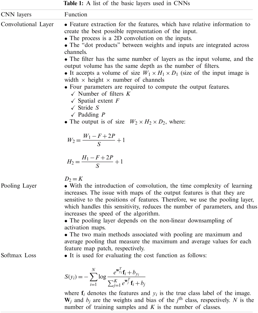
The classification task based on CNNs depends on several layers. Tab. 1 provides a list of the basic functions of a variety of CNN layers [5].

Rizzo et al. [8] presented a DNA classification approach that depends on a CNN, and the spectral representation of DNA sequences. From the results, they found that their approach provided similar and good results between 95% and 99% at each taxonomic level. Moreover, Rizzo et al. [1] suggested a novel algorithm that depends on CNNs with frequency chaos game representation (FCGR). The FCGR was utilized to convert the original DNA sequence to an image before feeding it to the CNN model. This method is considered as an expansion of the spectral representation that was reported to be efficient. This work is a continuation of the work of Rizzo et al. [1] for the classification of DNA sequences using a deep neural network, and chaos game representation, except for the addition of downsampling layers that can achieve the best trade-off between performance and time of processing, which is the main contribution of this work. The proposed approach is an improved form of the CNN to obtain better classification accuracy.

1.2 Data Reduction Step

A weakness of the convolutional layer performance is that it reports the exact position of features in the input. Slight shifts in the features located in the input image contribute to different feature maps. The pooling layer is used to resize the feature maps to overcome this problem. A simplified representation of the features observed in the input is the outcome of using a pooling layer. In practice, max-pooling works better than average pooling for computer vision fields such as image recognition [9]. We can handle this issue in signal processing by using downsampling methods such as 2D RP, two-Dimensional two-Directional Random Projection ((2D)2 RP)) and 2D DT. As a result, a lower-resolution representation of an input signal is produced, including the significant structural components without fine details that might not be helpful. The important purpose of the RP is to reduce the high dimensionality and preserve the geometrical relationship in the dimensionality reduction.

Dimensionality reduction methods can be briefly categorized into two classes, namely subspace and feature selection. Subspace methods include Principal Component Analysis (PCA), Linear Discriminant Analysis (LDA), Random Projection (RP), etc. The RP can be free from training and much faster. Some extensions of one-dimensional RP (1D RP), including two-dimensional RP (2DRP) [10], two-directional two-dimensional RP (2D)2 RP [11,12], sparse RP [13], require far lower computational complexity and storage cost than those of traditional 1D RP.

The authors of [13] used 2D schemes instead of 1D ones to reduce computational complexity and storage costs. In addition, in [10], the authors proposed (2D)2 PSRP methods to generate 2D cancelable faces and palmprints. The authors in [12] showed that 1D cancelable palmprint codes verification performance cannot meet the requirements of accuracy, and their computational and storage costs are large. So, 1D cancelable palmprint codes are extended to 2D cancelable palmprint codes. Moreover, the authors in [11] proposed a novel method called (2D)2 RP for feature extraction from biometrics, where they employed (2D)2 RP and its variations on the face and palmprint databases.

Feature selection methods depend on different spectral transformations such as two-dimensional Discrete Cosine Transform (2D DCT), and two-dimensional Discrete Wavelet Transform (2D DWT) to extract the features to reduce the amount of data, thereby simplifying the subsequent classification problem, and hence decision-making. Adaptive selection/weighting of features/coefficients is typically used for dimensionality reduction and performance improvement. The features that achieve high discrimination [14], high accuracy [15], and low correlation [12] should be selected and provided with high weights. The number of selected features is less than that of the original features. Feature selection methods have several advantages compared with subspace methods, such as PCA. Sometimes, feature selection methods can be fast and training-free, while it is comparable to the subspace methods in terms of accuracy. Furthermore, the selected features maintain their original forms. So, it is easy to observe the true values of the features. The authors in [16] proposed a novel approach for face and palmprint recognition in the DCT domain. In addition, the utilization of fusion rules is also an important tool to reduce computational complexity and storage costs [17].

The rest of this paper is organized as follows. Section 2 presents the proposed CNN models based on different downsampling layers. The max-pooling, DT, and RP are explained in Sections 3–5, respectively. Section 6 introduces the dataset. The results and discussions are given in Section 7. Finally, Section 8 gives the concluding remarks.

2  The Proposed CNNs Based on Different Downsampling Layers

We designed the proposed architecture, inspired by Rizzo et al. [1] architecture that has been reported as an efficient architecture for bacteria classification. We have added one convolutional layer followed by DT or 2D RP or variations~ of (2D)2 RP layer as compared to the original Rizzo et al. [1] architecture. Fig. 1 shows the proposed model. Firstly, the input DNA sequences are preprocessed using the FCGR algorithm with k = 6, 7, and 8. Thus, the output image is of dimension b0=4k×4k. For more details about FCGR, see [1,18]. Then, the normalized output is processed to make the input images suitable to the proposed CNN. The proposed CNN model consists of seven layers. The first four layers (from l1 to l4) are convolutional layers, each followed by a max-pooling layer. Additionally, the layers l5 to l6 are convolutional layers followed by various downsampling layers, which are applied to reduce the dimensionality of training. Several downsampling methods are implemented such as DT, 2D RP, and variations~ of (2D)2 RP. Simulation parameters are specified in Tab. 2.

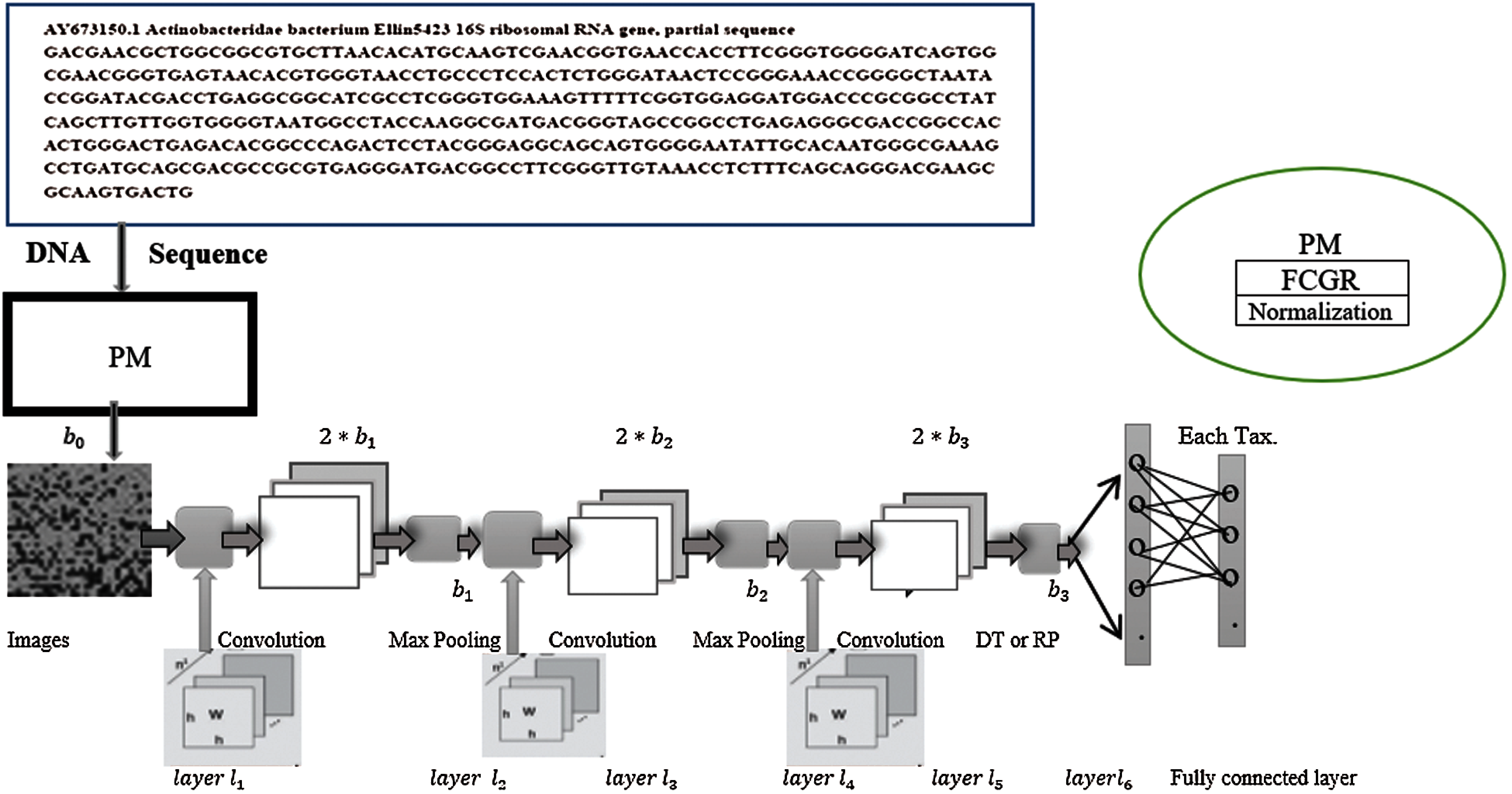
Figure 1: The architecture of the proposed model

After the convolutional layers, a set of the output images is generated; each of them of dimension (2bi+1), and:

bi+1=bi−y+12(1)

For example, let k = 6. Hence, b0=46×46=64×64, and the first convolutional layer (layer l1) produces 20 output images of dimension (64 – 5 + 1) = 60. Then, the pooling layer is applied, which produces 20 output images of dimension 60/2 = 30. The proposed CNNs are trained for five different classification tasks, as illustrated in Fig. 2, and the simulation parameters are presented in Tab. 2.

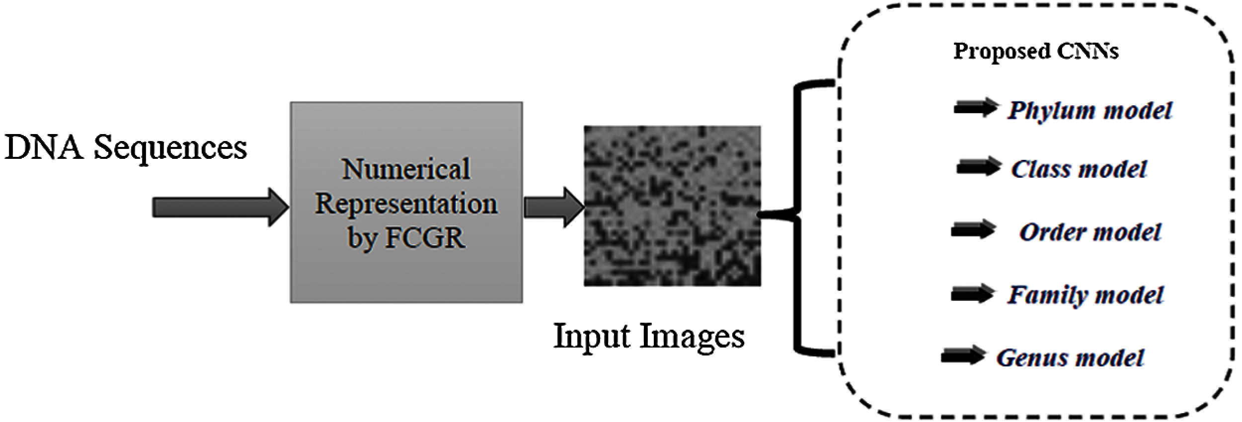
Figure 2: The architecture of the classifier

3  The Max-Pooling

The downsampling layer is another name for the pooling layer. It reduces the dimensionality of data, by dividing the input into rectangular pooling regions. The max-pooling computes the maximum of each region  Rij and consequently reduces the number of outputs. The max-pooling function is expressed as:

aij=max(p,q)∈Rij(apq)(2)

while the average pooling function can be expressed as:

aij=1|Rij|∑(p,q)∈Rij⁡apq(3)

where apq is the input at (p,q) within Rij , and |Rij| is the size of the pooling region.

Let us examine the effect of the max-pooling, when a 4 × 4 matrix input image is used, as shown in Fig. 3b.

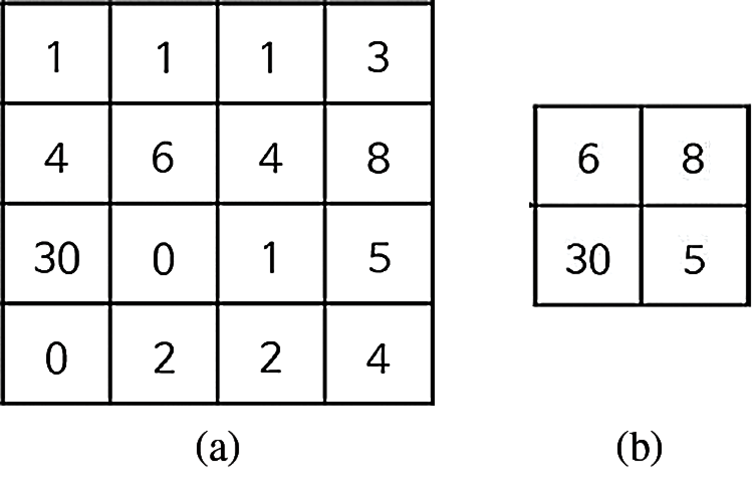
Figure 3: The pooling of a 4 × 4 matrix (a) The 4 × 4 matrix (b) The effect of max-pooling

In the case of an irregular nature of DNA sequences, k-mers recognition, the effective downsampling layer increases the ability of the CNN to achieve high performance. Anyway, the classification results do not critically depend on the feature extraction stage, but strongly depend on how these features are reduced.

4  Discrete Transform (DT)

Since the FCGR converts the DNA sequences into the form of images, we can apply the spectral transformations (Discrete Fourier Transform (DFT), Discrete Cosine Transform (DCT), and Discrete Wavelet Transform (DWT)) for downsampling, and the feature extraction stage for DNA images. The reason for applying these transformations emerges from their wide and effective use for extracting features, decorrelation, ordering, and dimensionality reduction purposes in the fields of speech, image, and bio-signal processing [19]. In signal processing, the DCT [20] can reveal the discriminative characteristics of the signal, namely, its frequency components. It is considered as a separable linear transformation. The basic idea of the DT is to select a certain sub-band after implementing the transformation. For example, the DCT can be implemented on the numerical sequence representing the DNA, and certain coefficients from the DCT can be selected to represent the whole sequence. The definition of the two-dimensional DCT for an input image A is given by:

Bp,q=αpαq∑m=0 M−1⁡∑n=0N−1⁡Amn cosπ(2m+1)p2Mcosπ(2n+1)q2N,     0≤p≤M−1 0≤q≤N−1(4)

where

∝p={1M,P=02M,1≤p≤M−1(5)

and

∝q={1N,q=02N,1≤q≤N−1(6)

while M and N are the row and column lengths of A, respectively.

The wavelet transform is faster and more efficient than the Fourier transform in capturing the essence of data [20]. Therefore, there is a growing interest in utilizing the wavelet transform to analyze biological sequences. The DWT is investigated to predict the similarity accurately and reduce computation complexity compared to the DCT and the DFT techniques.

The wavelet transform has been a very novel method for analyzing and processing of non-stationary signals such as bio-signals in which both time- and frequency-domain information are required. The wavelet analysis is often used for compression and de-noising of signals without appreciable degradations. The wavelet transform can be used to analyze the sequences at different frequency bands. In 2D DWT, the image is decomposed into four sub-bands. After filtering, the signal is downsampling by 2. In this work, the DWT is employed to reduce the dimensionality of features by performing the single-level 2D wavelet decomposition. The decomposition is conducted using a particular wavelet filter. Then, approximation coefficients (LL) can be selected. For example, let the first convolutional layer (layer l1) produce 20 output images of dimension  2b1. Then, a DWT pooling layer is applied, which produces 20 output images of dimension b1. Fig. 4 displays an example of the proposed DWT pooling.

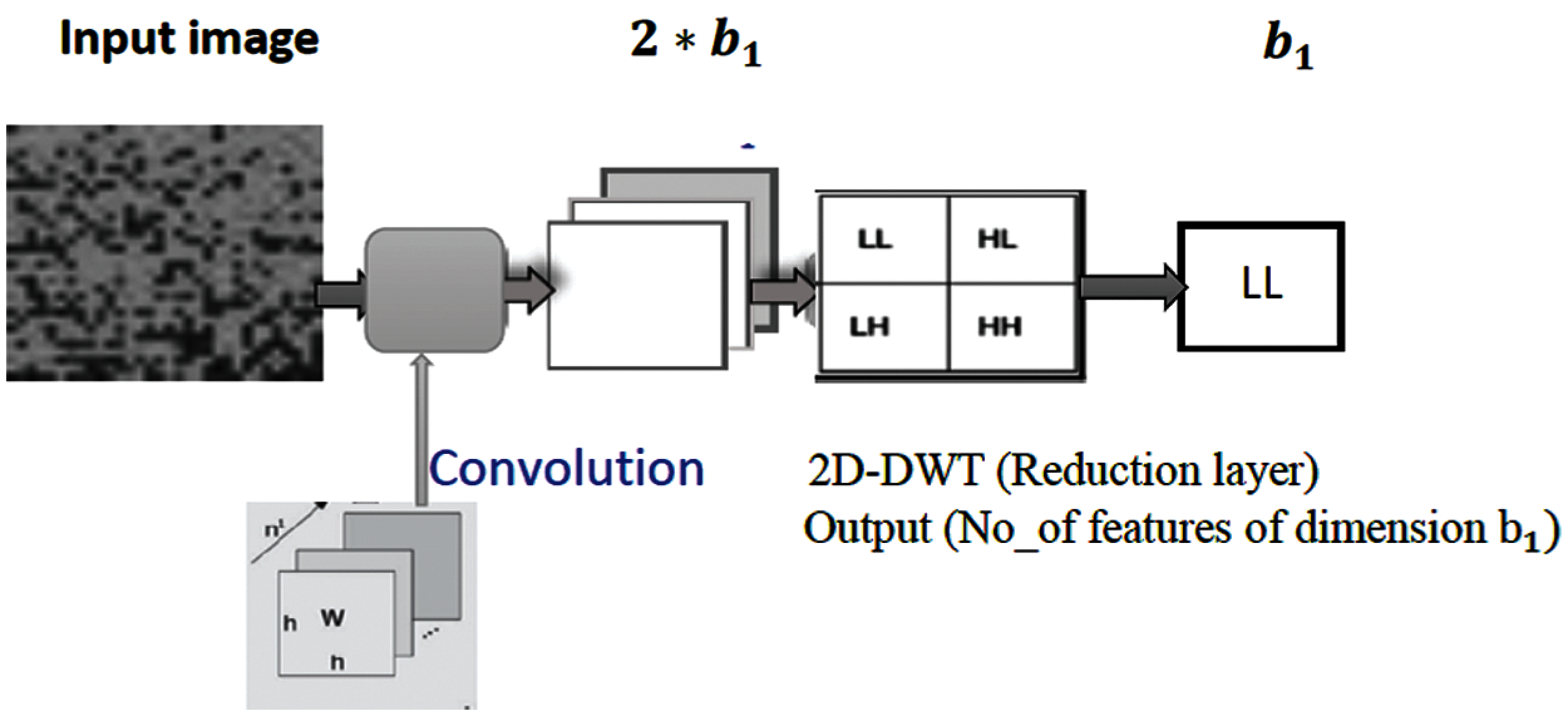
Figure 4: The proposed DWT pooling

5  Two-Dimensional Random Projection (2D-RP)

This method achieves the dimensionality reduction with low computational cost [21,22]. If the original dataset is represented by the matrix  Xd×n , then the projection of the data onto a lower k-dimensional space gives Yk×n~or~Y as follows:

Y=Yk×n=Rk×d.Xd×n(7)

where Rk×d is the RP matrix and k≪d.

5.1 Implementation of RP

The following stages of the RP are written using Matlab 2018a:

•   Set the input as the features map Xm×m (the multilayer CNN features).

•   Reshape the input to Xd×n.

•   Create a k × d random matrix (Rk×d), where k ≪ d.

•   for j = 1:n

•   Y(:, j) = R×X(:, j);

•   End for.

•   Output=Yk×n.

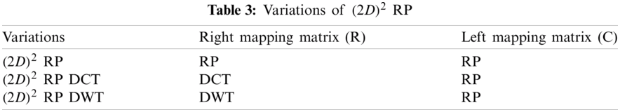
5.2 Two Directional Two Dimensional Random Projection (2D)2 RP

The 2D RP can be implemented simultaneously in two directions, that is called (2D)2 RP. In this method, the input matrix is projected at row direction and column direction as follows:

Y=Yk×h=Rk×d.Xd×n.Cn×h(8)

where R and C are the left mapping matrix for column-direction and right mapping matrix for row-direction, respectively and h ≪n, k≪d. The details of (2D)2 RP were explained in [12]. With Eq. (8), the projection of data onto a lower k and h dimensional subspace is implemented.

5.3 Variations of (2D)2 RP

The dimensionality reduction is the main purpose of pooling layers as introduced in the previous sections. In this work, the DWT and DCT are proposed to make the pooling layer to satisfy this purpose and add more details to feature maps. Hybrid methods that combine (2D)2 RP with DWT or DCT have been proposed. These methods are namely (2D)2 RP DWT and (2D)2 RP DCT based on the matrices R and C as indicated in Tab. 3.

 Y=Yk×h=Rk×dRP.Xd×n.Cn×hRP(9)

Y= Yk×h=Rk×dDWT.Xd×n.Cn×hRP(10)

 Y=Yk×h=Rk×dDCT.Xd×n.Cn×hRP(11)

6  Dataset Descriptions

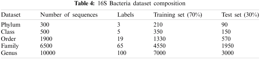
Data were obtained from the Ribosomal Database Project (RDP) [23], Release 11. A file in the FASTA record was obtained from the repository, which includes data on 1423984 outstanding bacterial gene sequences. For each bacterium, we have data on which taxonomic categories belong to certain genetic sequences. In addition, we have information on the phylum, class, order, family, and genus of a given 16S rRNA gene sequence. The bacterial genome contains the small-subunit ribosomal RNA transcript and is useful as a general genetic marker. It is often used to determine bacterial diversity, identification, and genetic similarity, and it is the basis for molecular taxonomy [24]. Two different sequences were used for comparison; (a) full-length sequences with a length of approximately 1200 – 1500 nucleotides and (b) 500 bp DNA sequence fragments. The total set of data includes sequences of the 16SrRNA gene of bacteria belonging to 3 different phylum, 5 different classes, 19 different orders, 65 different families, and 100 different genera, as shown in Tab. 4.

7  Results and Discussions

One of the key parameters that affect the DNA classification based on CNN is avoiding dimensionally problem and the sensitivity to the positions of the features. Even though the complex nature of DNA sequences is improved by convolutional layers, it is still necessary to ensure that the multi-layer CNN feature map has as suitable dimensions as possible. Therefore, there is a bad need to provide a downsampling layer that improves the generation ability of the original features. In this work, the CNN is utilized as a choice for deep learning, FCGR is applied for data preprocessing method, and different types of downsampling layers are introduced, such as DCT, DWT, 2D RP,  (2D)2 RP, (2D)2 RP DCT,~ and~ (2D)2 RP DWT. A comparison is presented for the performance of CNN based on different downsampling layers. Finally, a random search method is applied to optimize the hyperparameters.

7.1 Comparison between Different Types of Downsampling Based on CNN

The effectiveness of different downsampling layers has been investigated to classify bacterial sequences to reach the highest possible accuracy. First, the given DNA sequences have been mapped using the FCGR algorithm with k = 6, 7, and 8. Then, the proposed CNN models based on different downsampling layers have been trained for each taxon. These models are.

•   Model_1 (Max-CNN): Rizzo paper [1].

•   Model_2 (RP-CNN): CNN classification followed by max-pooling or 2D RP.

•   Model_3 (DWT-CNN): CNN classification followed by max-pooling or DWT.

•   Model_4 (DCT-CNN): CNN classification followed by max-pooling or DCT.

•   Model_5~ ((2D)2ZRP-CNN): CNN classification followed by max-pooling or (2D)2 RP.

•   Model_6 ((2D)2 RP DCT-CNN): CNN classification followed by max-pooling or (2D)2 RP DCT.

•   Model_7((2D)2 ZRP DWT-CNN): CNN classification followed by max-pooling or (2D)2 RP DWT.

To demonstrate the effectiveness of the proposed models, two simulation experiments are conducted. In the first case, the efficiency of the prediction for each taxonomic level is measured separately by taking into account the whole bacteria sequence. In the second case, instead of the whole sequence, we consider only the 500 bp long sequences. The simulation results are demonstrated in Tabs. 5–7, and Fig. 5 introduces the experimental results for the full-length DNA sequences, while Tabs. 8–10 and Fig. 6 present the results for 500 bp-length sequences. The classification is obtained for the same sequence with the representation of images at different values of k. From these tables and figures, it is clear that the proposed CNN model based on DWT and (2D)2 RP DWT always achieves the best performance. Furthermore, the (2D)2 RP DWT-CNN model consumes less running time. The best choice for mapping is at k = 8, because it improves the accuracy and F-score compared with those achieved at k = 6 and 7. Moreover, the proposed CNN based on (2D)2 RP DWT has a processing time that is less than that of the max-CNN by about 135 sec on average. From the mentioned results, the proposed (2D)2 RP DWT-CNN model with k equal to 8 provides superior results compared with other models.

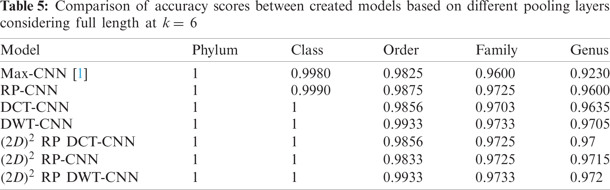
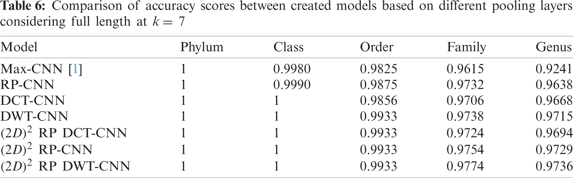
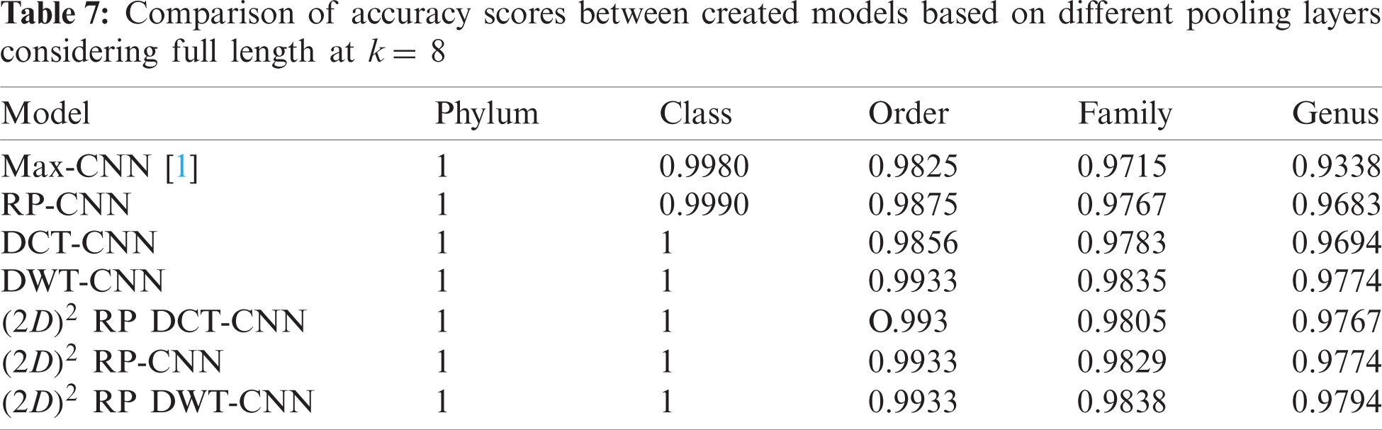
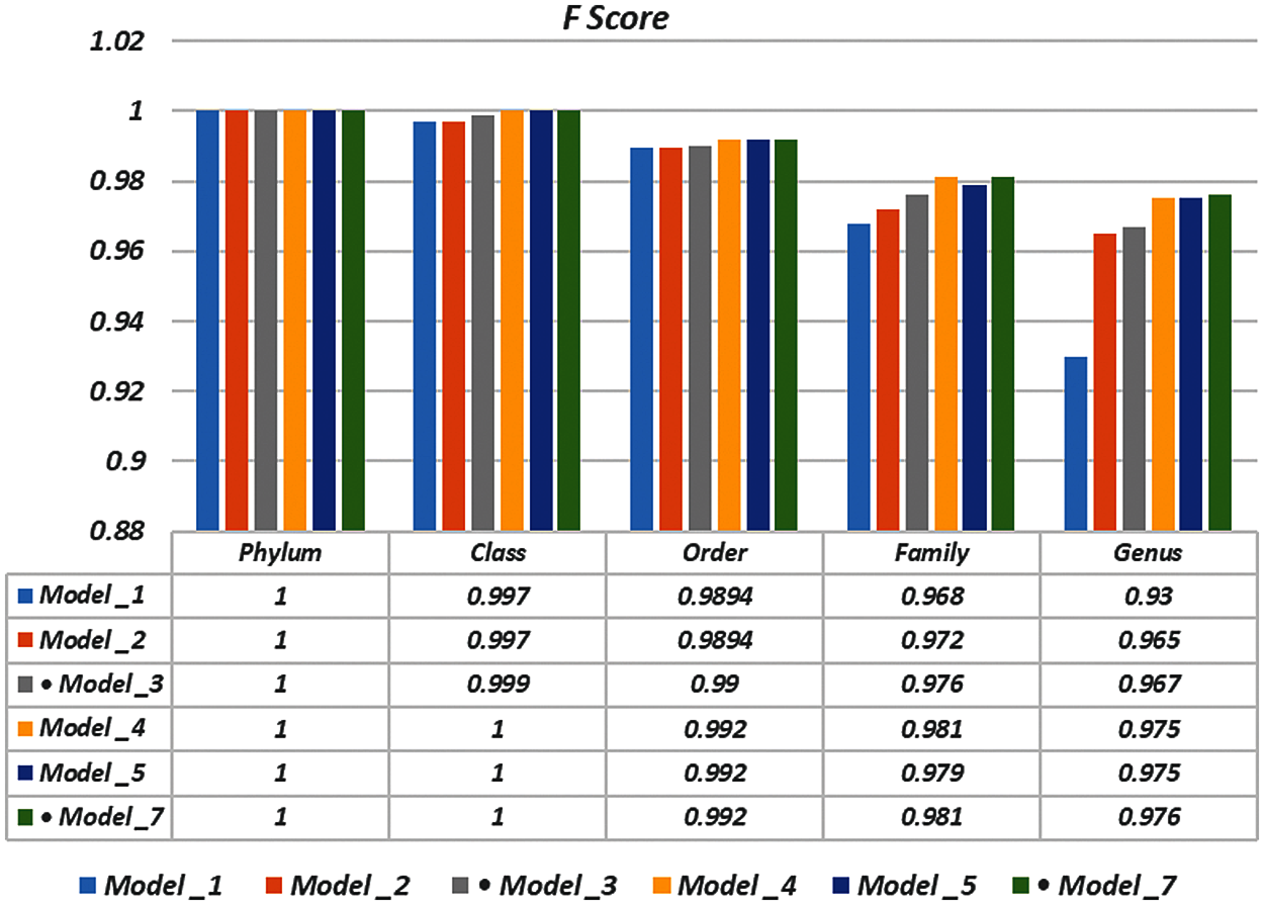
Figure 5: F-scores of the proposed model at k = 8, for the full length case

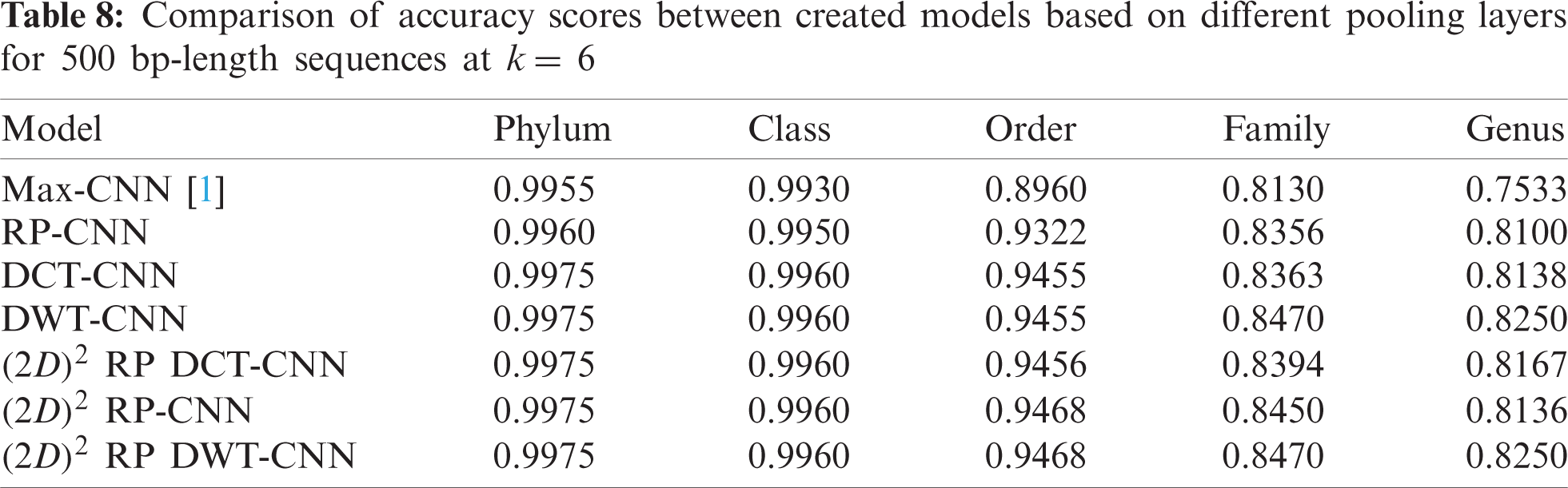
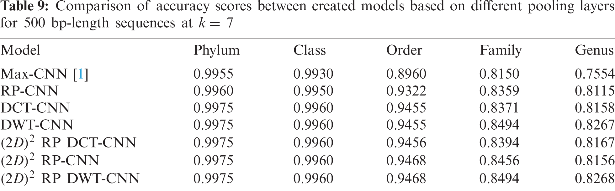
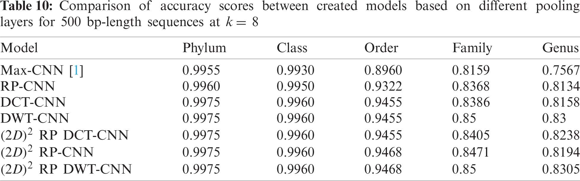
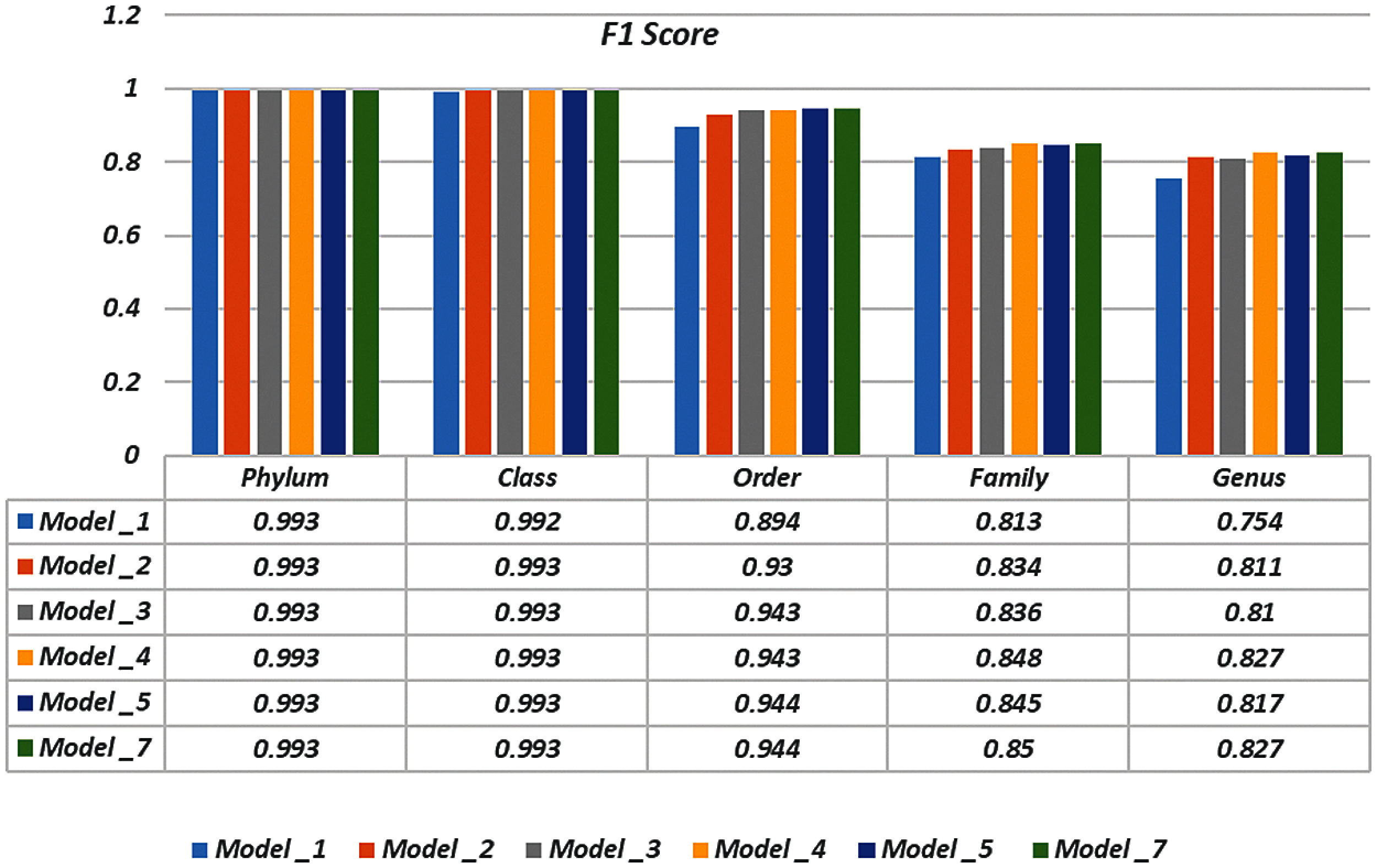
Figure 6: F-scores of the proposed model at k = 8, for 500 bp-length sequences

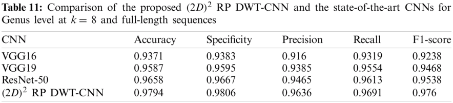
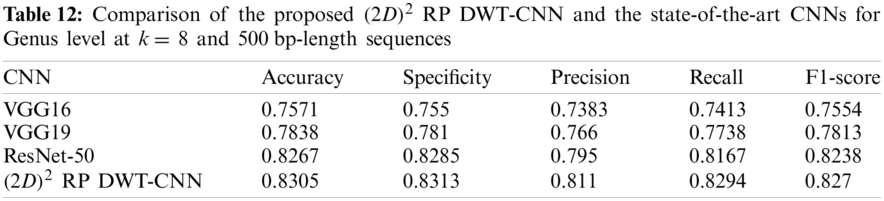
Tabs. 11 and 12 present comparisons between the performance of the proposed (2D)2 RP DWT-CNN and the state-of-the-art models; VGG16, VGG19, and ResNet-50 at k = 8 and different DNA sequences using the full-length and 500 bp-length sequences, respectively. The results indicate that the proposed (2D)2 RP DWT-CNN achieves better accuracies at the genus level, by about 4.23% and 7.34% compared to the VGG16 model for the full-length and 500 bp-length sequences, respectively. The proposed model consumes 53 min, which is the lowest computational time compared to the VGG16, VGG19, and ResNet-50. For VGG16, VGG19, and ResNet-50, the computational times were recorded as 62, 87, 134 min, and also they have lower accuracies of classification. Finally, a comparison is conducted among the proposed ((2D)2 RP DWT-CNN model and the mentioned state-of-the-art models based on different datasets for the three most popular taxonomic trees (RDP, SILVA, and green genes) [24].

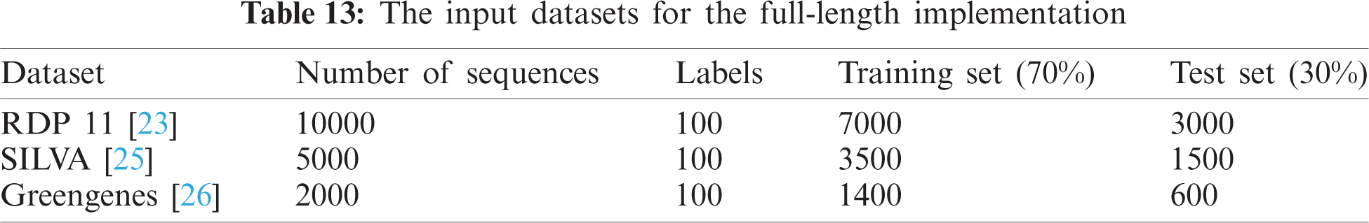
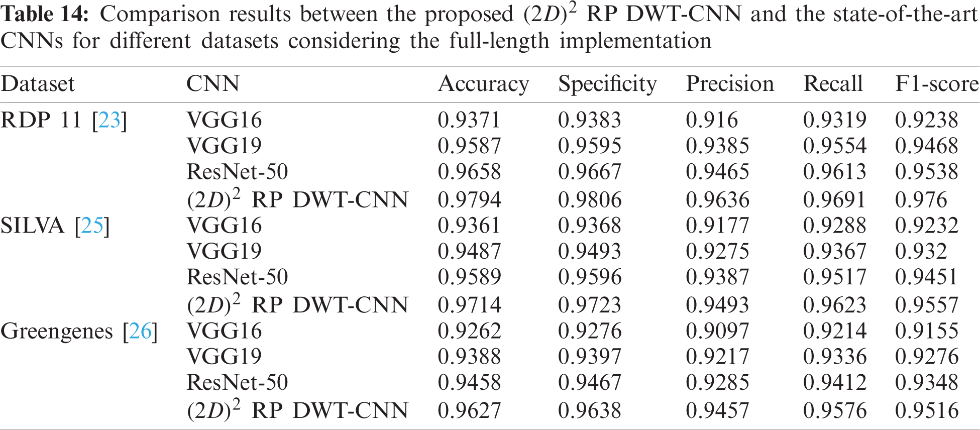
Tab. 13 indicates the different datasets used for the full-length implementation. Tab. 14 summarizes the experimental results for the proposed model and the state-of-the-art models. It is shown that the proposed model is superior, and it achieves a classification accuracy equal to 97.94% against 97.14%, 96.27%, and 96.27% for RDP 11, SILVA dataset [25], and greengenes dataset [26], respectively.

7.2 Hyperparameter Tuning

The training process may be quite difficult due to the enormous number of initial variables called hyperparameters. These values are defined before the start of the learning process. Some examples of hyperparameters include the learning rate, the minibatch size, and the number of epochs. In this paper, some changes in hyperparameters are applied to iteratively configure and train the proposed model. This section can be divided into subsections as follows:

7.2.1 Learning Rate Results

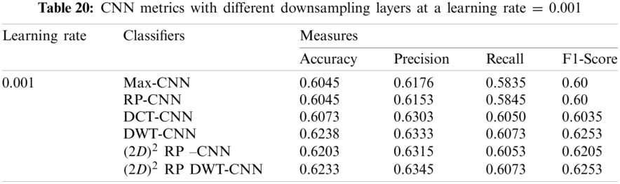
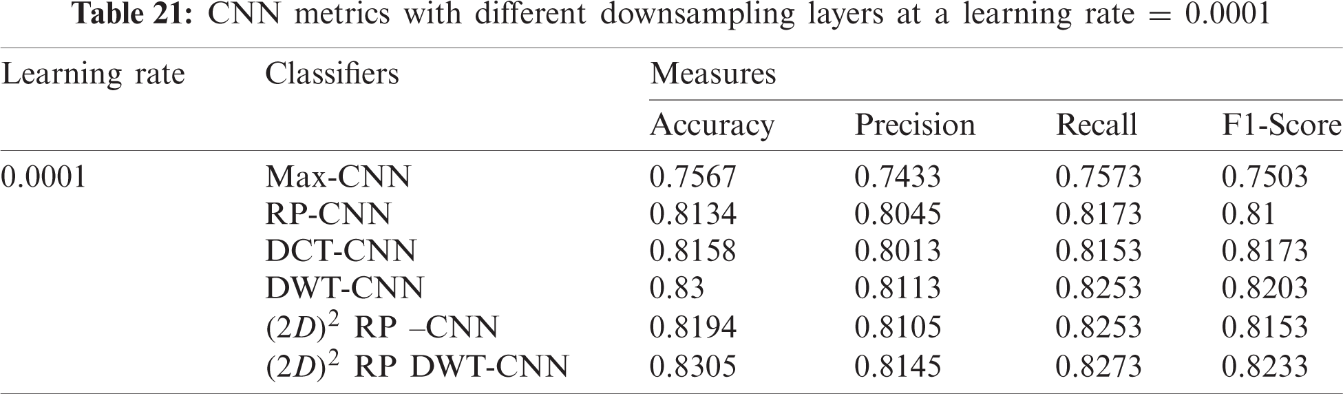
In this subsection, the effect of the learning rate on the CNNs with different downsampling layers at the genus level is investigated in the case of full-length and 500 bp-length sequences. These downsampling layers include Max-CNN, RP-CNN, DCT-CNN, DWT-CNN, (2D)2 RP DCT-CNN, (2D)2 RP-CNN and (2D)2 RP DWT-CNN. The parameters used in the simulation are mini-batch with 64, and the number of epochs for training is equal to 20. The comparison among the mentioned models at different learning rates is shown in Tabs. 15–18 for the full-length sequences.

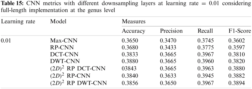
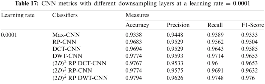
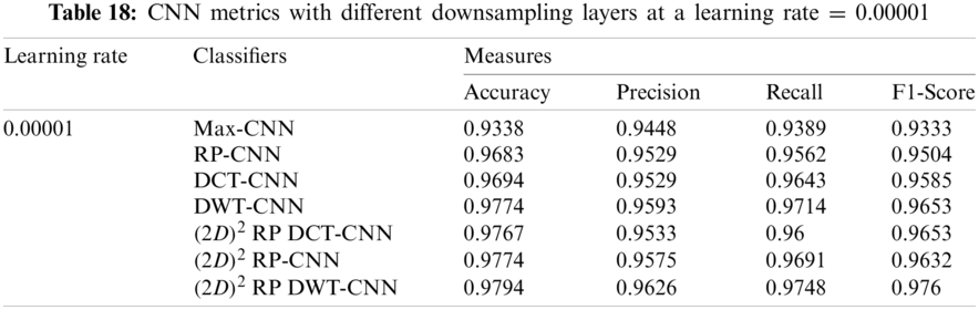
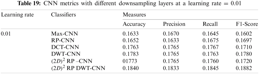
It can be noted that the highest accuracy is obtained at the learning rate equal to 0.0001 and 0.00001, but processing time increases, where 0.0001 learning rate has a processing time less than that of the 0.00001 learning rate. The same comparison is conducted for 500 bp-length sequences to trust the achieved results as demonstrated in Tabs. 19–21. Therefore, at a 0.0001 learning rate, superior accuracy for the training set can be attained for any length of the DNA sequences.

7.2.2 Mini-batch Size and Number of Epochs

In this subsection, the evaluation using different mini-batch sizes is investigated in the training process against different iterations for the proposed (2D)2 RP DWT-CNN model (at genus level considering full-length implementation) with the number of epochs = 20 and the learning rate equal to 0.0001. The experimental results are illustrated in Fig. 7. It is clear at mini-batch size equal to 128, the proposed (2D)2 RP DWT-CNN achieved less accuracy performance, while at mini-batch sizes equal to 32 and 64, the proposed model has a better trade-off between the accuracy score and the processing time.

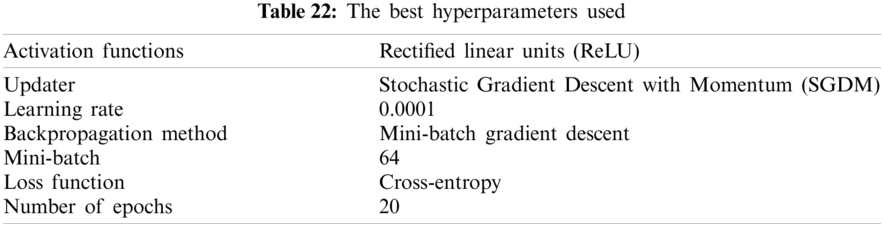
From the mentioned results, we can conclude that the best performance of the proposed DWT-CNN model is achieved at the learning rate equal to 0.0001 and the mini-batch size equal to 64. We can select a suitable number of epochs considering these values. Fig. 8 reveals the training progress of (2D)2 RP DWT-CNN model at k equal to 6 considering the full-length implementation at a different numbers of epochs. It can be observed that best accuracy is obtained at 20 epochs. Finally, after several experiments, we give the best hyperparameters in Tab. 22.

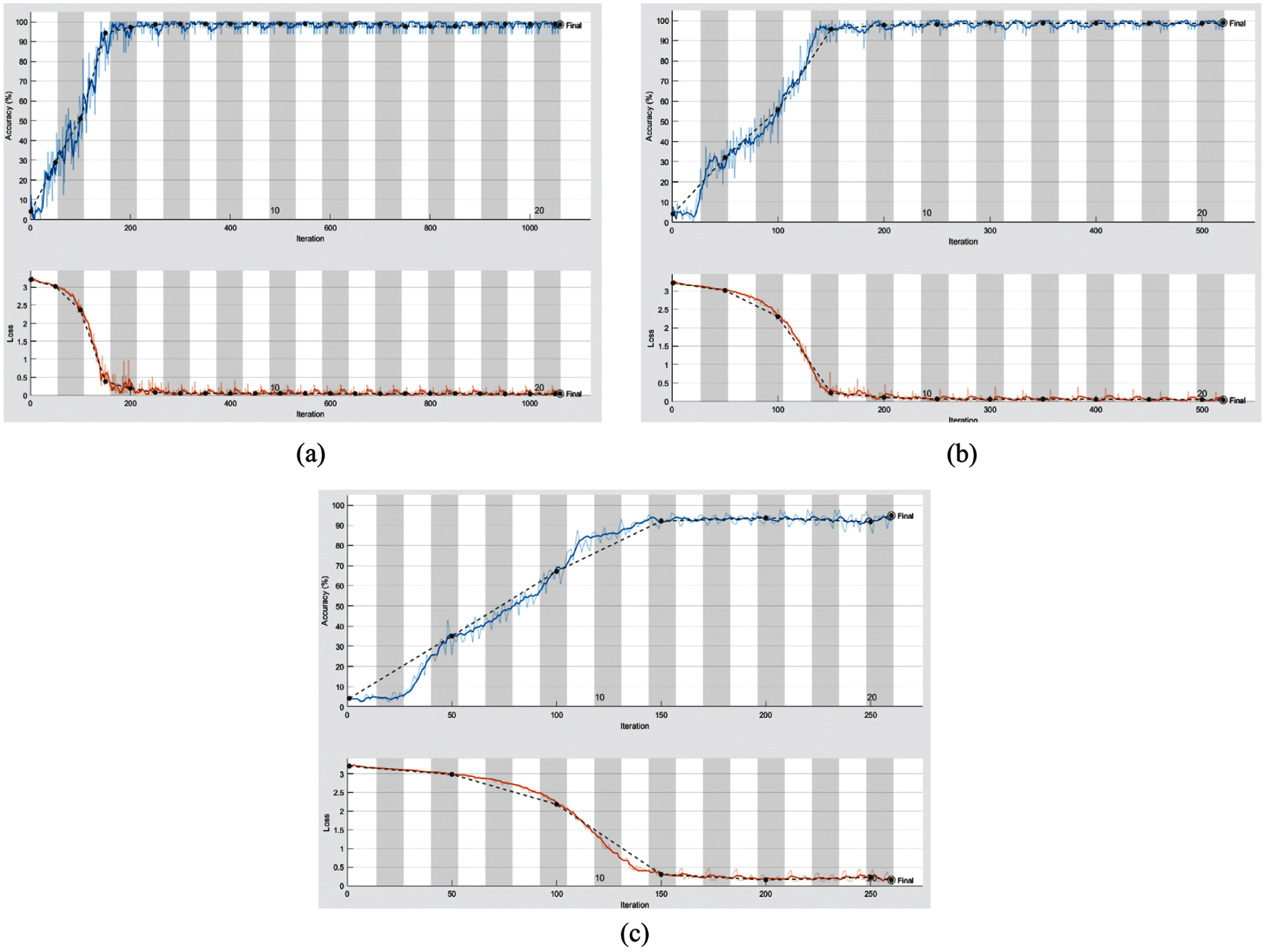
Figure 7: Training progress of (2D)2 RP DWT-CNN model (k = 6) considering full-length implementation at different mini-batch sizes (a) 32, (b) 64, and (c) 128

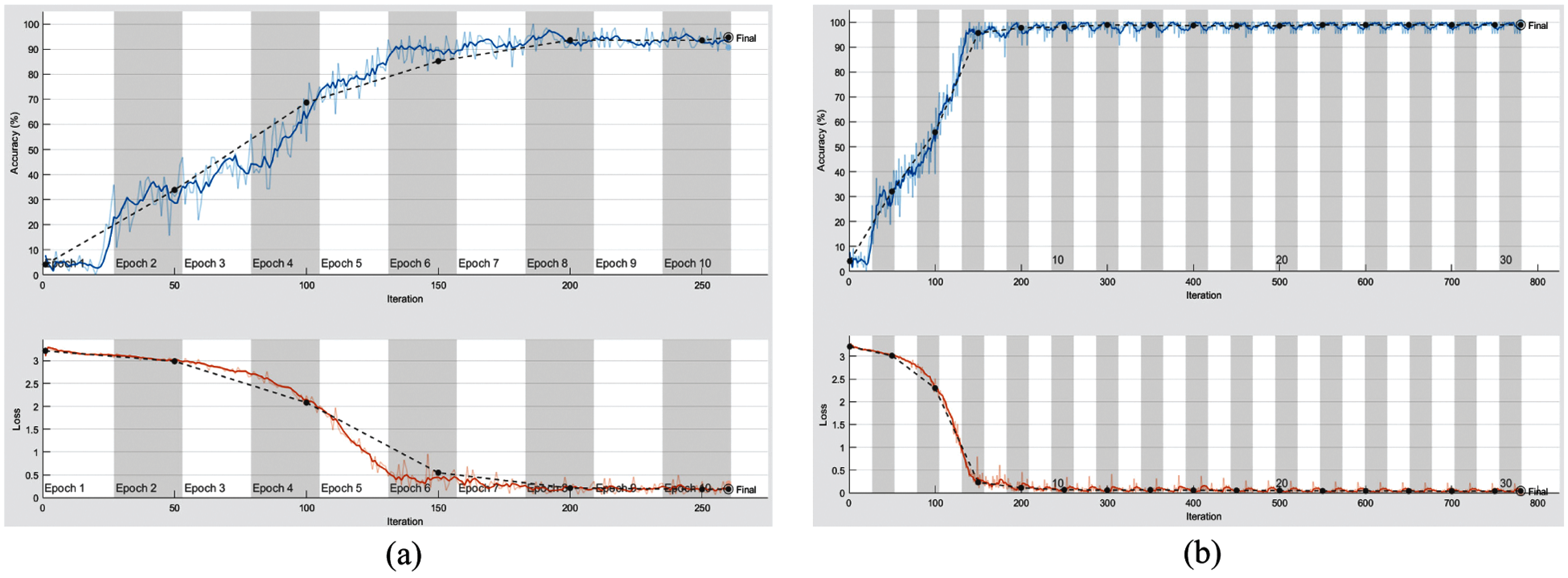
Figure 8: Training progress of (2D)2 RP DWT-CNN model (k = 6) considering full-length implementation at different numbers of epochs (a) 10 and (b) 30

8  Conclusions and Future Research Directions

This paper presented two contributions to the bacterial classification of DNA sequences. The first one is represented in the proposed models for bacterial classification using an improved CNN. In these models, the 2D RP, (2D)2 RP,~ (2D)2 RP DCT, (2D)2 RP DWT, and DT methods are applied to reduce the dimensionality of the feature maps, while preserving the structure information. The proposed models make the data reduction process faster and more reliable. The simulation results revealed that selecting the appropriate downsampling layer with the training CNN could greatly influence the accuracy with an optimized computational time. According to the obtained results, it can be concluded that the CNN based on (2D)2 RP DWT gives a high accuracy. Furthermore, this model can achieve a good trade-off between the accuracy score and the processing time for a suitable size of the frequency k-lengthen words in DNA sequences. Finally, the experimental results on different datasets reveal that the proposed (2D)2 RP DWT model outperforms the state-of-the-art CNNs models. The second contribution lies in evaluating the effectiveness of the hyperparameters through the created CNNs based on different downsampling layers to select the best results. It is possible to say that the best accuracy is provided by using (2D)2 RP DWT as a downsampling layer with k = 6. This study confirms that with a learning rate equal to 0.0001, the mini-batch size equal to 64, and the number of epochs equal to 20 are suitable to achieve the best performance on the given DNA dataset. For future work, the performance of different frequency-domain transforms for DNA classification can be investigated. In addition, deep CNN models developed from scratch can be designed to improve the DNA classification efficiency.

Acknowledgement: The authors would like to thank the support of the Deanship of Scientific Research at Princess Nourah Bint Abdulrahman University.

Funding Statement: This research was funded by the Deanship of Scientific Research at Princess Nourah Bint Abdulrahman University through the Fast-track Research Funding Program.

Conflicts of Interest: The authors declare that they have no conflicts of interest to report regarding the present study.

This work is licensed under a Creative Commons Attribution 4.0 International License, which permits unrestricted use, distribution, and reproduction in any medium, provided the original work is properly cited.