DOI:10.32604/cmc.2022.019135
| Computers, Materials & Continua DOI:10.32604/cmc.2022.019135 | |
| Article |
A Non-Destructive Time Series Model for the Estimation of Cherry Coffee Production
1Telematics Engineering Group, University of Cauca, Popayán, 190002, Colombia
2INRAE, University of Toulouse, UMR 1248 AGIR, F-31326, Castanet Tolosan, France
3Department of Software Engineering, University of Granada, Granada, 18071, Spain
*Corresponding Author: Jhonn Pablo Rodríguez. Email: jhonnpablo@unicauca.edu.co
Received: 03 April 2021; Accepted: 07 May 2021
Abstract: Coffee plays a key role in the generation of rural employment in Colombia. More than 785,000 workers are directly employed in this activity, which represents the 26% of all jobs in the agricultural sector. Colombian coffee growers estimate the production of cherry coffee with the main aim of planning the required activities, and resources (number of workers, required infrastructures), anticipating negotiations, estimating, price, and foreseeing losses of coffee production in a specific territory. These important processes can be affected by several factors that are not easy to predict (e.g., weather variability, diseases, or plagues.). In this paper, we propose a non-destructive time series model, based on weather and crop management information, that estimate coffee production allowing coffee growers to improve their management of agricultural activities such as flowering calendars, harvesting seasons, definition of irrigation methods, nutrition calendars, and programming the times of concentration of production to define the amount of personnel needed for harvesting. The combination of time series and machine learning algorithms based on regression trees (XGBOOST, TR and RF) provides very positive results for the test dataset collected in real conditions for more than a year. The best results were obtained by the XGBOOST model (MAE = 0.03; RMSE = 0.01), and a difference of approximately 0.57% absolute to the main harvest of 2018.
Keywords: Cherry coffee; production estimation; learner; approaches; time series; weather data; crop management data
Smart or Precision Agriculture (PA) refers to information and technology-based agricultural management systems (e.g., remote sensing, geographic information systems, global positioning systems, or robotics) for a more efficient soil and crop management based on their identified or estimated conditions [1]. The application of PA can be beneficial at all scales and levels of agricultural development [2]. Crop yield prediction is a key objective of PA to achieve a more precise and accurate use of operations and resources considering georeferenced information, and monitored characteristics of soil, plant, and climate, thus reducing costs and waster, and increasing the quality of the final product. Recent advances in sensor technologies, Big Data, Internet of Things (IoT), Artificial Intelligence (AI) and machine learning approaches has shown a great potential to advance PA and achieve accurate predictions [3–5].
According to the International Coffee Organization (ICO) [6], coffee is the second most consumed beverage worldwide after water. Currently, Brazil, Vietnam and Colombia are the biggest exporters of coffee in the world [6]. In Colombia, coffee plays a priority role in the generation of rural employment (there are more than 547 thousand coffee growers and 853 thousand hectares of coffee planted [7]). The importance of coffee production is evidenced in the economic and social level. For instance, in Colombia around 540,000 families depend on coffee production as income source [6,7]. In addition to the indirectly related sectors such as commerce, finance and the informal economy that revolves around this activity. The department of Cauca is one of the most relevant regions in coffee production, with more than 93,000 coffee growing families and generating 65,500 agricultural jobs [8].
Due to the importance of coffee crops in Colombia, coffee growers must estimate the production of cherry coffee beans to support decision-making in planning activities, number of workers required, necessary infrastructure, anticipated negotiations, and losses of coffee production in a given territory [8]. Accurate predictions of crop yield are critical for developing effective agricultural and food policies at the regional and global scales. Currently, Colombian coffee growers estimate cherry coffee production based on direct field measurements [9], which may cause losses in their production and generate extra costs for the collection of samples. Usually, the sampling process consists of selecting 60 coffee trees per hectare, from which the coffee beans are extracted and subsequently weighted [9]. Due to the complexity and costs of the sampling process, only a very reduced number of samples and corresponding data corpora are available, which leads to inaccurate measures with high error rates in cherry coffee production estimation. The cherry coffee beans that constitute the sample are discarded from the coffee production chain, which generates additional losses to the coffee growers, and so we refer to this approach as “destructive”.
Different approaches have been proposed to estimate crop production by means of machine learning approaches in tomato, sugar cane, wheat, corn crops, etc. [4–5,10]. However, these proposals exclude weather and crop management information, besides they are focused on crops different than coffee. In this paper, we propose a non-destructive model for the estimation of cherry coffee production based on sensor variables, time series and machine learning (ML) algorithms. Weather and crop management information sources are considered to improve the accuracy of the estimators. The evaluation results show that that the algorithms based on regression trees (XGBOOST, TR and RF) provide accurate crop yield estimations for a realistic test dataset collected in real conditions, thus providing a solution within the framework of precision agriculture to develop expert systems to estimate cherry coffee production.
The remainder of the paper is structured as follows. Section 2 describes related approaches to crop production estimation. Section 3 presents our proposal for estimating cherry coffee production and the combination of variables, machine learning approaches and dataset used to learn the proposed models. Sections 4 and 5 describe the evaluation process and the results obtained. Finally, Section 6 presents the conclusions and suggests some future work guidelines.
Farmers have traditionally relied on their own experiences and past historical data (e.g., crop yields and weather) to make decisions to increase short-term profitability and long-term sustainability [11–13]. During the last years, machine learning approaches have emerged as a key element in precision agriculture for farmers and agronomists’ to make better informed choices [2,11]. This section describes the main ML approaches related to the estimation of production in different crops, the main methods that are proposed, and key conclusions extracted.
The model proposed in [14] used two datasets collected from 1983 to 2013 with the weather characteristics (temperature, rainfall, and humidity) and the production of the rice crop of three coastal districts belonging to the region of Odisha in India. The AdaBoost algorithm is proposed to predict rice production by means of the combination of the results obtained by a set of statistical models: linear, lasso, crest, and support vector regression (SVR) machines. The MAE (Mean Absolute Error), MSE (Mean Squared Error), MAD (Mean Absolute Deviation) and R-Squared errors are considered to estimate the predictive quality of the proposed methods.
Gonçalves et al. [4] proposed a multiple linear regression (MLR) model to estimate sugarcane production in the state of São Paulo (Brazil). Their proposal is based on time series considering meteorological and agroclimatic data. The proposed model uses variables related to planted area, normalized difference vegetation index (NDVI) and water requirement satisfaction index (WRSI), which presented correlation coefficients around 0.90. In addition, the results of the evaluation showed a directly proportional relationship between sugarcane production and NDVI, and inversely proportional to WRSI.
Qader et al. [5] combined MODIS (Moderate Resolution Imaging Spectroradiometer Spectrum Radiometer) satellite imagery data with crop production information to develop a statistical model to forecast winter wheat and barley production in Iraq. From the satellite image information, the authors calculated the vegetation indices (NDVI and EVI, enhanced vegetation index). The best result was obtained with the NDVI vegetation index.
Fernández-Mensaque et al. [15] presented an approach for olive crop forecasting based on airborne olive pollen counts, meteorological observations and agronomic practices. This study was conducted in Campiña Alta, Córdoba (Spain). Data from different information sources was combined and four linear regression were obtained to forecast the crop 6 months with varying degrees of reliability. The equation
Garg et al. [16] used historical wheat yield data from the Odisha University of Agriculture and Technology in India to forecast wheat yield from mathematical equations of degree from 1 to 4. They classified the wheat yield variable into 7 fuzzy intervals (very poor yield, poor yield, not so good yield, average yield, good yield, very good yield, excellent yield). The authors obtained the lowest MSE (Mean Squared Error) with a third-degree cubic equation (MSE = 180.98).
Sujatha et al. [17] proposed an architecture for crop yield prediction that includes an input module for considering the farmer's opinion. The input module considers the crop name, land area, soil type, soil pH, pest details, climate, water level, seed type. The selection module selects the subsets for each attribute. Then, a crop yield prediction model is used to predict plant growth and plant diseases. After entity selection, a classification rule is used to group similar contents. A regression model for yield prediction is used with variables related to the variety, crop area, soil type, soil pH, pest control, water level, seed type. Finally, they perform variable selection by grouping climatic data and crop parameters.
Ramesh [18] described two techniques for crop prediction (MLR multiple linear regression and DBC density-based clustering). These models were evaluated in the East Godavari district of Andhra Pradesh (India). The following input variables were considered for the models: year (date of data capture), rainfall, sowing area, yield, fertilizer (nitrogen, phosphorus, potassium) and crop yield. The results obtained showed a 2% difference between the actual value and the predicted values.
Oliveira et al. [19] presented a machine learning-based system that uses data from multiple sources to perform soybean and corn yield forecasts. The system consists of a recurrent neural network (RNN) trained with variables of rainfall, temperature, soil and historical soybean or corn production. The proposal was evaluated in regions of Brazil and USA. The coefficient of determination was defined as evaluation measure, obtaining values from 0.55 to 0.75 with the proposed system.
Zhang et al. [20] predicted wheat yield in several regions of China using linear regressions from land cover data, production data (wheat, corn, soybean and rice yields), NDVI, auxiliary information (administrative boundaries, crop calendar and geographical distribution). Analytical indicators are extracted from the NDVI of the time series. Then, linear regressions with the rest of features. The prediction error is lower than 8% and they also obtain a coefficient of determination of 86.6%.
Kerdiles et al. [21] presented a tool called CST (Crop Statistics Tool), which allows predicting crop yields using historical crop management data and meteorological or remote sensing data, from multiple regression analysis or scenario analysis (attempts to identify the most similar years to the current one). The results of the evaluation showed that maize yields in Ethiopia are highly correlated with vegetation rainfall in the region of Oromiya. The tool obtained an R²-adjusted value for 4 zones close to or above 90%.
Sun et al. [22] implemented simple linear models using remote sensing data to forecast rice crop yield in Hubei (China). They compared the actual crop yield from statistical data with the model results. The results indicated that the error ranges from −14.38% to 11.31% compared with the actual data, and the correlation coefficient was 0.87.
Lee et al. [23] presented a nonparametric regression model for agricultural yield forecasting, that was evaluated on apple crops in Korea. The model is based on 33 years of monthly climate data (maximum temperature, minimum temperature, average temperature, rainfall, and sunshine hours) and crop production data. The model obtained a Mean Absolute Percentage Error (MAPE) of 5.71e-12 and an R-squared of 1 for the prediction of the crop production for a specific month.
A gray model (GM) and an autoregressive integrated moving average (ARIMA) model are implemented in [24] to predict grain crop yields from yield data for the years 1998 to 2008. They performed the predictions for the years from 2009 to 2013 and obtained an average error of 7.88% (GM) and 12.32% (ARIMA), and an average accuracy of 92.12% and 87.68% respectively. The GM model provided the best results for grain crop yield prediction.
Rale et al. [25] described the use of several linear and nonlinear regression models with cross-validation to predict wheat yield in different counties in the United States. The dataset used involved 2 years of county geolocation variables, climate data, vegetation indices and the target variable wheat yield. The best results were obtained using the Random Forest model, with an R² value of 0.83, an RMSE of 5.30, and a mean absolute percentage error of 5%.
Gamboa et al. [3] predicted cocoa crop yield through a set of photosynthetic, morphological, climatic, chemical and physical variables (obtained from 2015 to 2017). Two models were evaluated: Generalized Linear Model (GLM) and Support Vector Machines (SVM). The results of the evaluation of these models at La Suiza research center in Rio Negro, Santander (Colombia) showed that the trunk diameter, phosphorus, magnesium, radiation, temperature, humidity, and accumulated rainfall were the more significant variables to explain the yield of the cocoa crop. The model providing the highest accuracy was the Generalized Linear model, which obtained a
Mayer et al. [26] predicted crop production of macadamia nuts in six regions of Australia. A set of crop variables (tree age, variety, region, and tree spacing) and climatic variables (maximum and minimum temperature, evaporation, solar radiation, rainfall, modeled transpiration efficiency, water stress and modeled soil-water index) was considered for the study. Cross-validation was used to demonstrate that LASSO regression models with MAE errors <10% outperformed general linear models and partial least squares regression (PLS regression).
The combination of the previously described ML techniques and deep learning methodologies have been proposed when labeled training data are scarce. Tedesco-Oliveira et al. [27] have recently developed an automated system with convolutional networks (CNN) for cotton yield prediction from using color images taken by a smartphone. The proposed models have been trained with images acquired at different times during the day. Three scenarios (low, medium, and high demand computational resources) are defined for the evaluation. The proposed system obtains an error of 17.86% in predicting performance using 205 images from the test partition.
There are few studies describing the estimation of production in coffee crops, since all the research that has been done so far is focused on the detection of diseases, such as rust [28]. Ramos et al. [29] developed a computer vision system for counting coffee beans on tree branches. The authors used a dataset of 1,018 images of coffee tree branches at different stages of maturation. The system was validated in four plots of Castillo variety coffee, at different stages of development and different densities, with a correlation higher than 90% in the early stages of crop development.
Rodríguez et al. [30] have recently proposed a computer vision approach to detect cherry coffee beans in crops. Their proposal is based on images captured by a mid-range smartphone in an uncontrolled environment. The image set used in this study contained images of the entire coffee plant of 3 coffee varieties (caturra, bourbon, and castle). The system achieved the best results for bourbon coffee plants with a 0.59 accuracy and 67% of the total relevant cherry beans correctly classified.
Kouadio et al. [31] evaluated an Extreme Learning Machine (ELM) model to analyze soil fertility properties (soil organic matter, potassium, boron, sulfur, zinc, phosphorus, nitrogen, exchangeable calcium, magnesium, and pH) and generate an accurate estimate of robusta coffee yield. Compared to Multiple Linear Regression and Random Forest models, the ELM model contributes to the proper selection of the significant soil properties that can be used in coffee yield. The proposed ELM model considering organic matter, potassium and sulfur characteristics as predictor variables generated the most accurate coffee yield.
With this review it has been possible to identify that crop estimation is one the main problems linked to production, for which different artificial intelligence techniques and learner algorithms have been proposed to calculate estimates. The research proposals described in this section are focused on yield or production estimation in different crops (corn, cotton, rice, etc.) considering different information sources and artificial intelligence techniques (computer vision, machine learning, deep learning, etc.). However, the reduced number of proposals described for coffee crops can be considered just initial approximations to the estimation of coffee production.
This section describes the dataset, the time series and the learners used to create the non-destructive time series model.
Crop management information and weather data were used to build time series models. Below, dataset and data preprocessing are explained.
The coffee crop dataset was provided by Supracafé,1 from the farm “Los Naranjos” located in Cajibio, Colombia (21°35′08″N, 76°32′53″W). The farm is composed by 38 plots (Fig. 1). Each plot contains the following information: plot ID, coffee variety, crop age, density, control activities, fertilization activities, cleaning activities, geolocation (latitude, longitude, altitude), altitude above sea level, and cherry coffee production during the years 2012, 2013, 2014, 2016, 2017, and 2018. The year 2015 was not considered due missing values presented in crop management variables.
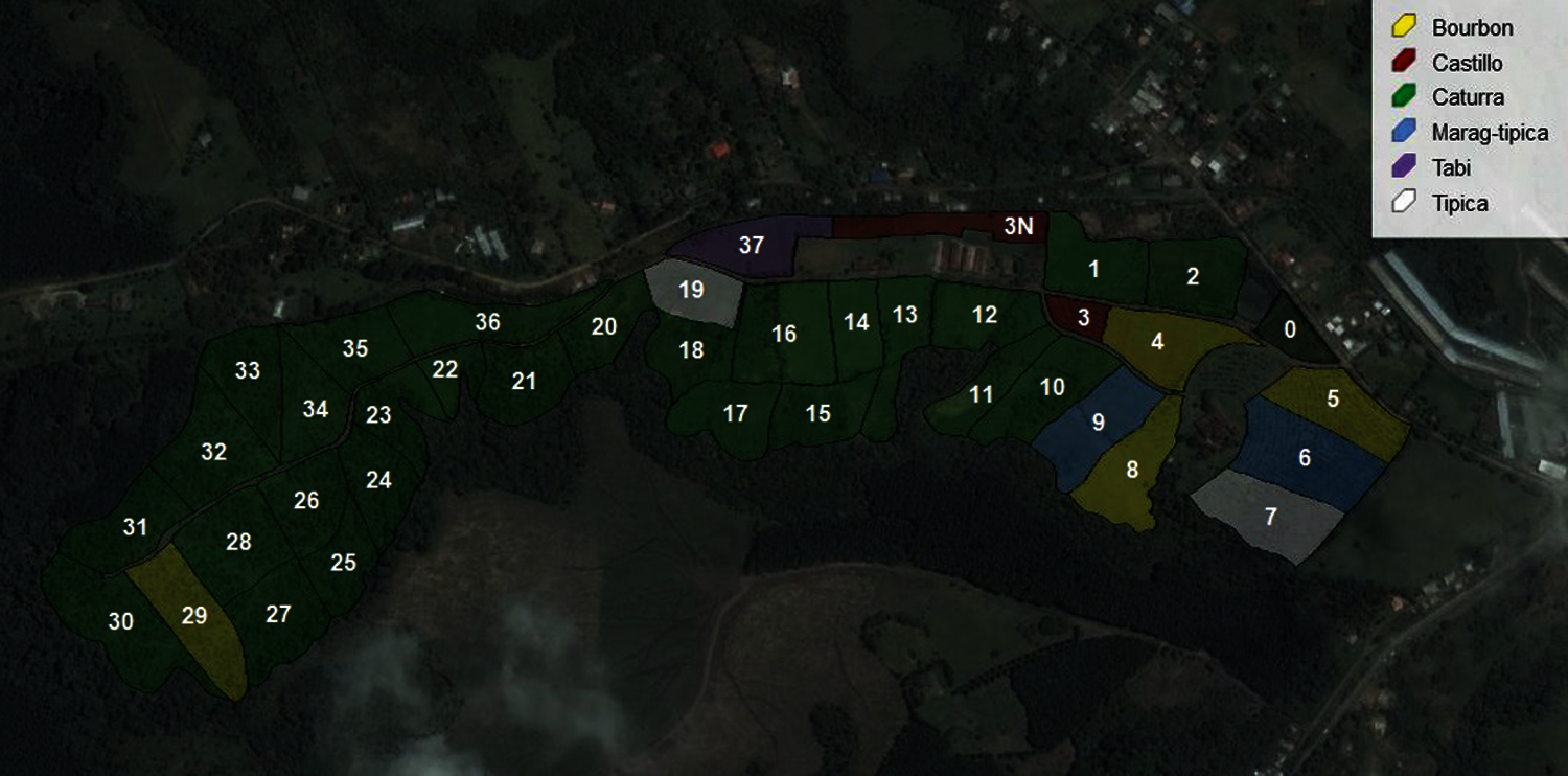
Figure 1: Plot distribution of the Naranjos farm [32]. Numbers in white color correspond to plot ID
The weather data was provided by Meteoblue2 (Meteorological Service created at the University of Basel, Switzerland, in cooperation with the National Oceanic and Atmospheric Administration of the United States and the National Centers for Environmental Prediction) during 2012 to 2018. Due to the missing values presented in crop management variables for 2015, the weather data for 2014 was discarded because weather data influence the coffee harvest of following year. Weather data consists of 4 variables with hourly time scale: temperature, relative humidity, precipitation, and solar radiation.
The datasets of crop management and weather were merged and subsequently, we defined three time series based on expert knowledge by agronomists of TECNICAFE.
3.2.1 Monthly Time Series (MTS)
The crop management variables as control, fertilization and cleaning were defined in the most influential periods of the main coffee harvest, i.e., for the months November, December, and February as Tab. 1 shows.
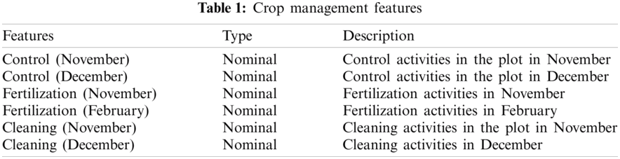
In addition, we added the monthly temperature of the maximum (Max_Temp), minimum (Min_Temp) and mean (Avg_Temp) values from 6 am to 6 pm. The STM time series were built for each plot, for a total of 37 models.
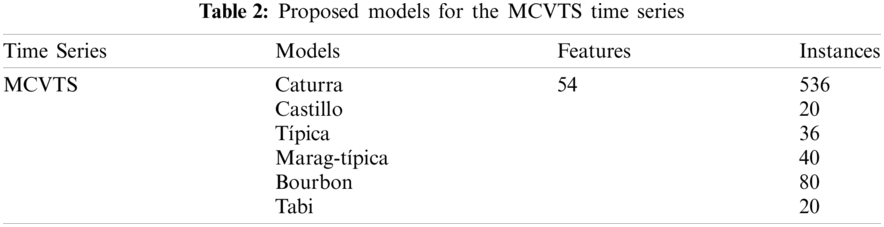
3.2.2 Monthly Coffee Variety Time Series (MCVTS)
MCVTS was sorted by coffee variety. Six models (Tab. 2) were trained with around 20–536 instances and the same variables of the MTS.
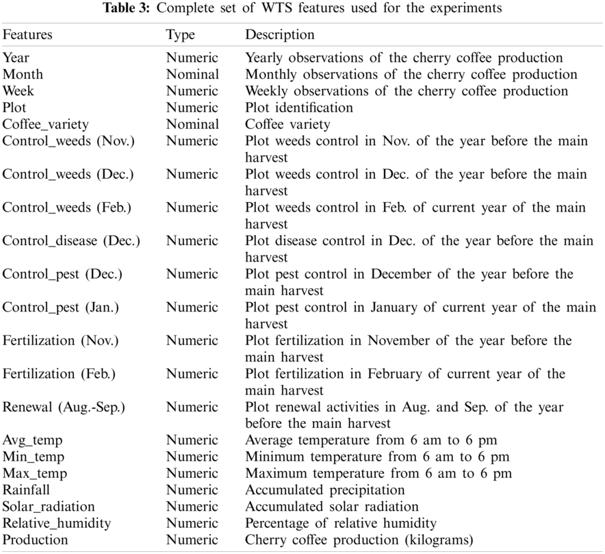
3.2.3 Weekly Time Series (WTS)
WTS corresponds to weekly data (318 variables and 107 instances). Additional data was integrated from weekly by the entire farm. For instance, the production of cherry coffee for MTS contains the amount in kg collected by month. In WTS, cherry coffee production represents the amount in kg collected by week. Therefore, we approximately increase instances of the dataset from 1 to 4. New crop management attributes were generated according to the information provided by agronomist from the coffee farm.
MTS variables of crop management (control, fertilization, and cleaning) were processed to calculate new attributes, such as weeds control, disease control, pest control, renewal, and fertilization. In addition, crop management variables were modified from nominal to numerical values; they were computed as the number of occurrences per control management category performed during that week, as shown in Tab. 3.
This section describes the learners used for the estimation of cherry coffee production. We used six learners: Tree Regression (TR), Linear Regression (LR), Artificial Neural Networks (ANN), Extreme Gradient Boosting (XGBOOST), Random Forest (RF) and Support Vector Regression (SVR).
In addition, two additional feature selection methods were used to improve the results: a Pearson Correlation filter method (PC) and Recursive Feature Elimination [33]. The PC filter method uses Pearson's correlation to select the best subset of variables from highest absolute value of correlation between an independent and dependent variable. We define a Pearson correlation <= 0.2 as threshold. RFE selects a subset of variables starting with all features in the training dataset and successfully eliminating features until the best quality prediction is achieved. The XGBOOST algorithm was used for RFE.
This section presents the experiments performed using the three-time series described in Section 3.2. Six experiments were defined from processed dataset and feature selection methods as Tab. 4 shows. The E-01 experiment considers all the features of the MTS with monthly time scale. To increase the number of instances and features in the dataset, the MCVTS time series was constructed to perform the E-02 experiment with the implementation of the learners considering all the features. For the E-03 experiment, we used WTS time series which organizes the data on a weekly time scale. E-03 and WTS increases the number of instances (107) and features (318) used in previous experiments. Due to the poor results obtained in E-01 and E-02 experiments with the LR algorithm, it was decided that the LR algorithm should be discarded in the following experiments, and the XGBOOST and RF algorithms were added.
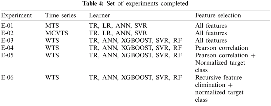
In the E-04 experiment, we applied a feature selection method with aim to decrease the dataset high dimensionality. A Pearson correlation criterion was used to select the relevant of features based on highest correlation between each dependent variable and the independent variable. From experiment E-04, to reduce the values of the evaluation metrics, the target variable was normalized to complete the E-05 experiment (i.e., the production of cherry coffee is transformed in such a way that the values are between 0 and 1); this ensures that the target variable is within a range. Finally, the E-06 experiment further decreases the dimensionality of the data set by considering the normalized objective variable. For feature selection, the Recursive Feature Elimination technique succeeded in reducing the set of features to only 51.
This section presents the results obtained for the set of experiments described in the previous section. The evaluation measures used to validate the models were [34]: Mean Absolute Error (MAE), Root Mean Squared Error (RMSE), and Relative Squared Error (RSE). In addition, the tests carried out for E-01, and E-02 experiments were with the information of the years 2012–2014, 2016, as a training set and the year 2017 as a test suite. Instead, for E-03, E-04, E-05, and E-06 experiments, the training set was l to information from the years 2012–2014, 2016, 2017, and the test suite was the year 2018.
Tab. 5 shows the results of the evaluation metrics for the first experiment (E-01). The best results were obtained by the TR algorithm due to the small sample size of the data set. Regression trees perform better than the rest of algorithms.
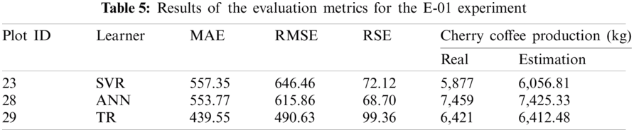
Fig. 2 shows the best result obtained by the TR algorithm for the plot 29. The difference of the actual total production of the 2017 main crop with respect to the estimated one was only of 8.5 kg. However, the values of the estimated production for each month present a greater difference.
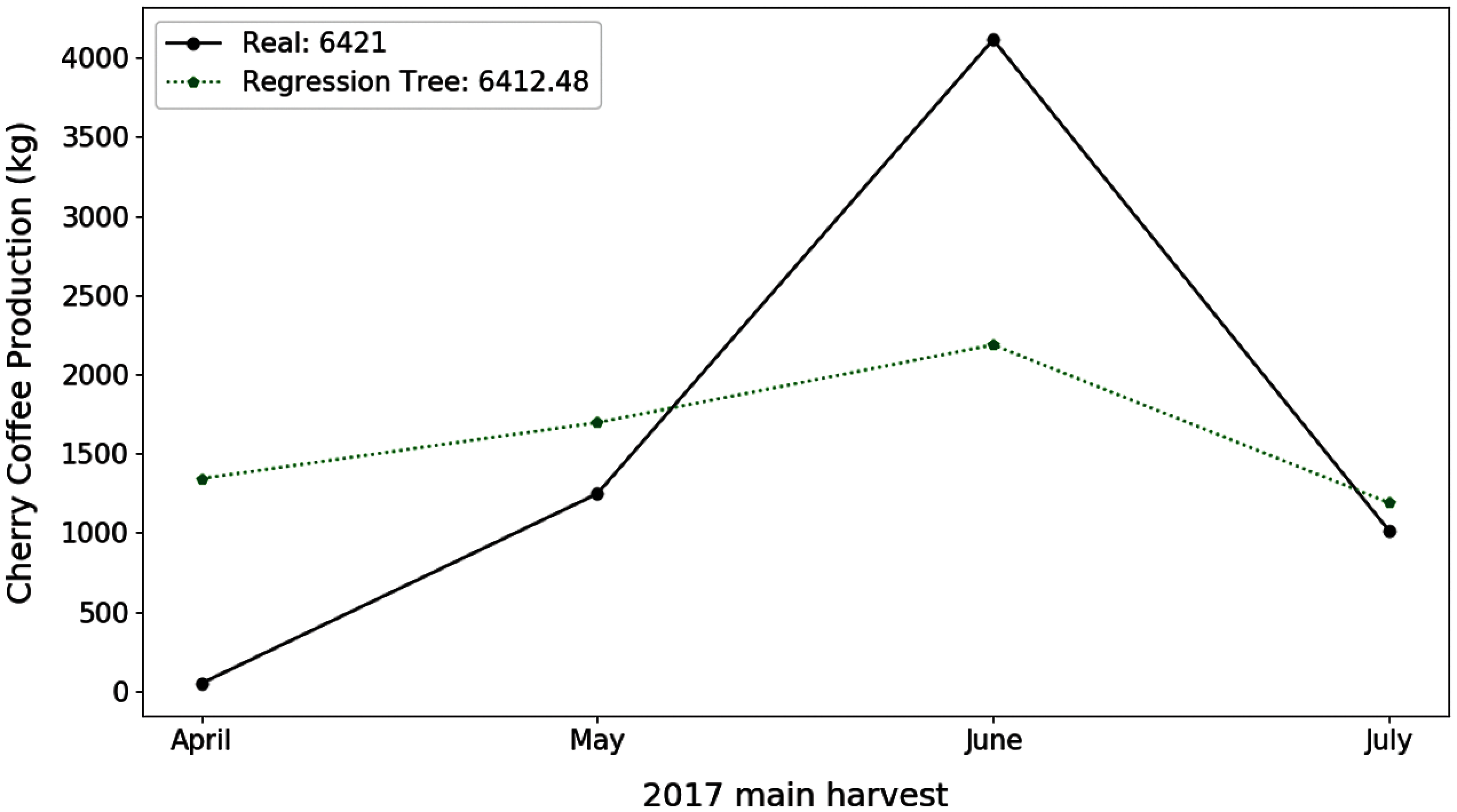
Figure 2: Estimation of coffee production by means of the E-01 experiment. On the x-axis are the months corresponding to the main coffee harvest of the year 2017. And on the y-axis the amount in kg of cherry coffee production
For the E-02 experiment, the TR and ANN algorithms provided the best results compared to the SVR and LR algorithms (Tab. 6). The models created for the bourbon and castle varieties increased the samples, which made the TR algorithm to obtain satisfactory results for these metrics. The use of ANN models also provided satisfactory results even for the models trained with few samples (Tabi, Marag-typica). As Fig. 3 shows, the best result for this experiment was obtained with the ANN algorithm in the time series of the caturra variety for plot 28. The difference between the estimate and the actual production of each month decreased with respect to the E-01 experiment. However, when calculating the total harvest, the total difference was greater (33.60 kg).
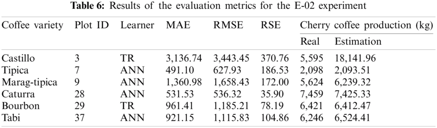
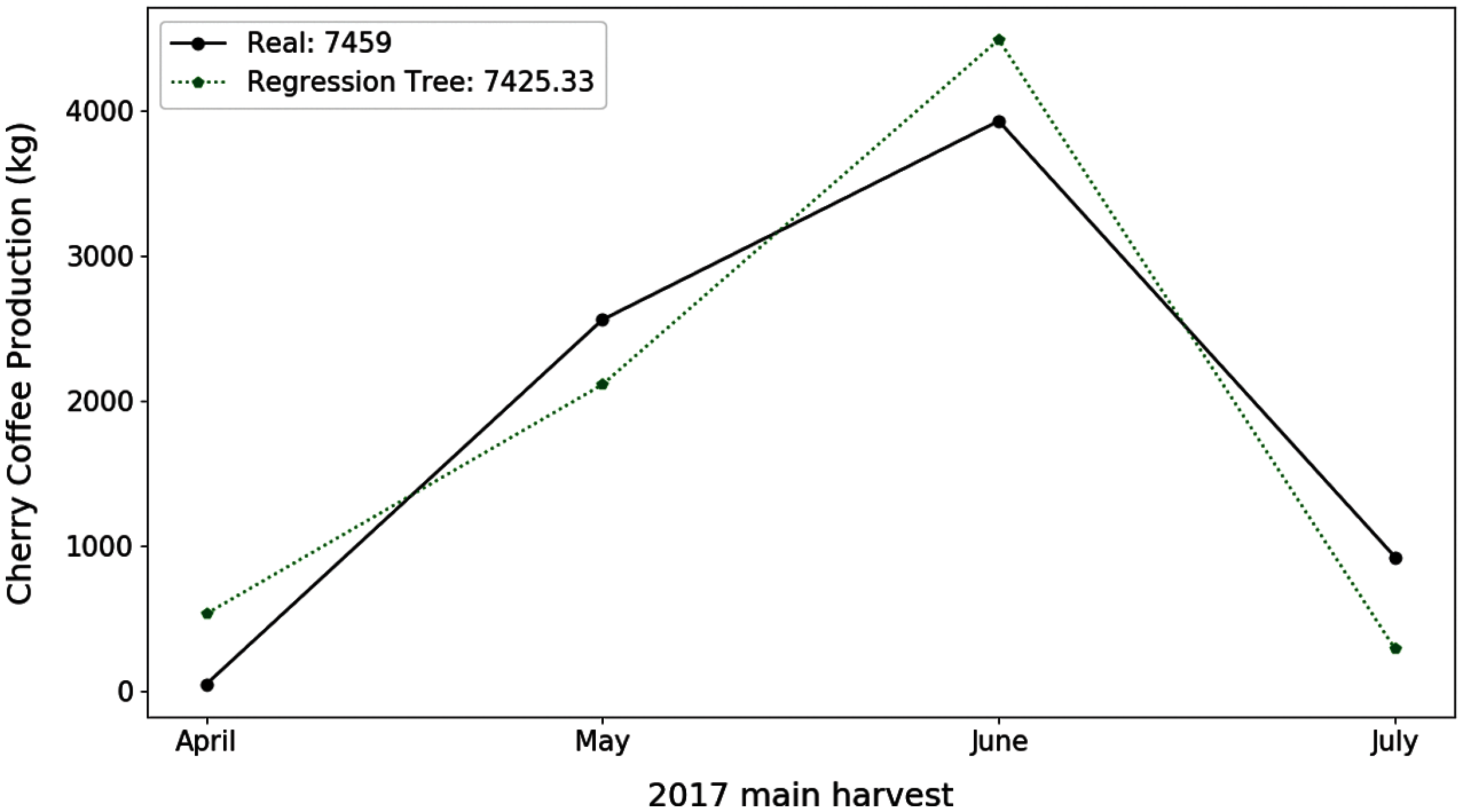
Figure 3: Estimation of coffee production by means of the E-02 experiment. On the x-axis are the months corresponding to the main coffee harvest of the year 2017. And on the y-axis the amount in kg of cherry coffee production
The XGBOOST and RF algorithms did not improve the results described for the E-01 and E-02 experiments in subsections 5.1 and 5.2.
The XGBOOST and RF algorithms were evaluated in the E-03 experiment given their widespread use for similar tasks. The LR algorithm was discarded due to its weak results obtained in the E-01 and E-02 experiments. Tab. 7 shows that the XGBOOST and RF algorithms provide the smallest difference of the estimation of the actual total production.
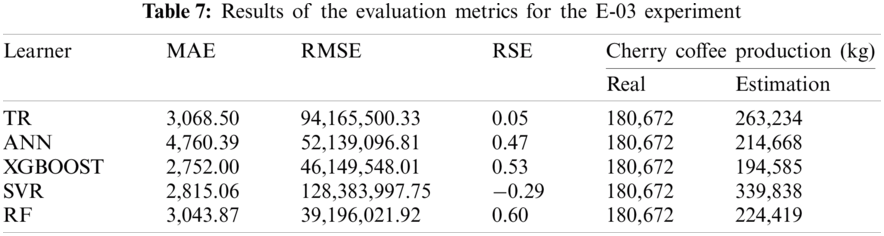
Fig. 4 shows the estimates provided by the XGBOOST and RF algorithms, which are more similar to the main harvest curve for 2018. The ANN and SVR algorithms, on the other hand, provide results that are higher than the expected values of coffee production. Finally, the TR algorithm provides results below the curve.
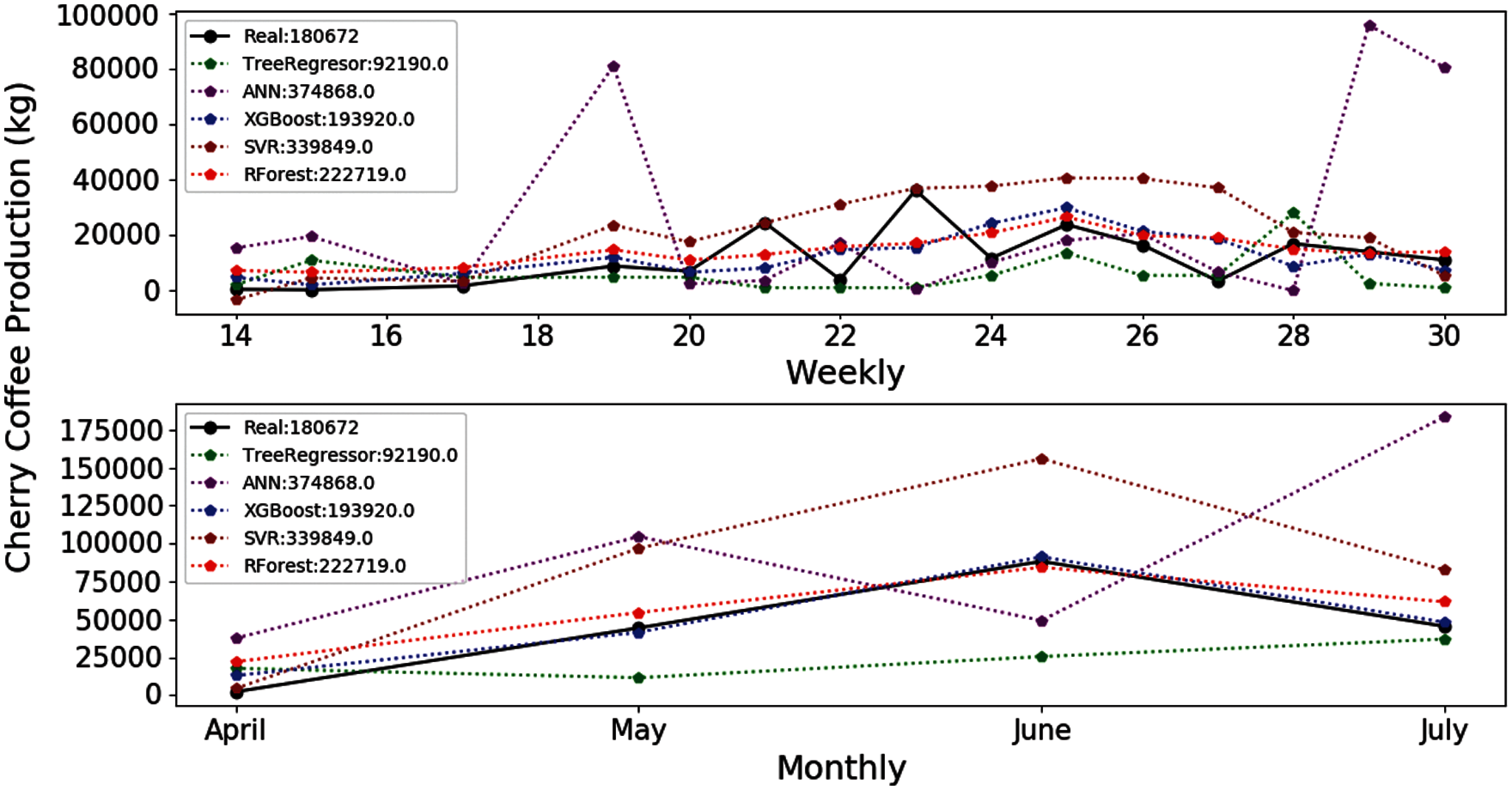
Figure 4: Estimation of coffee production by means of the E-03 experiment. On the x-axis are the months corresponding to the main coffee harvest of the year 2018. And on the y-axis the amount in kg of cherry coffee production
The E-04 experiment uses a reduced number of features of the initial set. The results of the evaluation metrics for the XGBOOST and RF algorithms are also better than the results provided by the rest of algorithms. However, the MAE, RMSE and RSE errors are still very high (Tab. 8). In addition, the TR algorithm improved its results using fewer features than in the previous experiment. Fig. 5 shows that the estimates of the algorithms improve regarding the E-03 experiment. In addition, less information is needed for their training. However, the estimates generated by XGBOOST and RF still provide the best results for the main 2018 harvest productions.
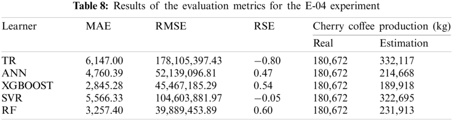
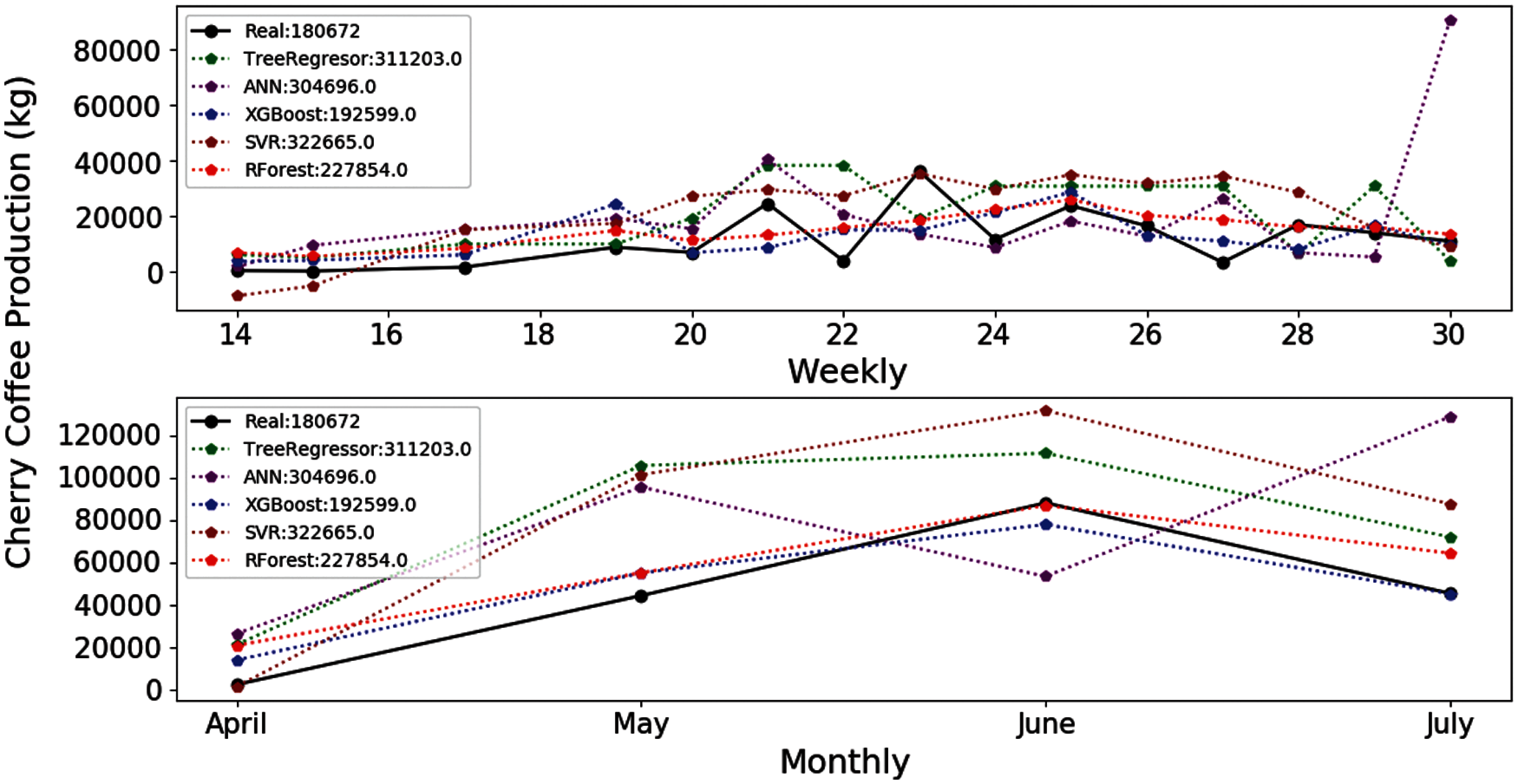
Figure 5: Estimation of coffee production by means of the E-04 experiment. On the x-axis are the months corresponding to the main coffee harvest of the year 2018. And on the y-axis the amount in kg of cherry coffee production
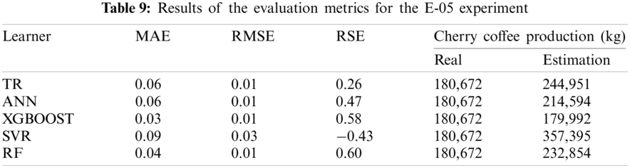
The values of the evaluation metrics decreased considerably in the E-01, E-02, E-03 and E-04 experiments. However, the XGBOOST and RF algorithms also outperform the rest of learner techniques in the E-05 experiment. The estimates of the 5 learner algorithms (except SVR) improve regarding the previous experiments. The results obtained by the XGBOOST algorithm are very close to the real production considered in the main harvest of 2018 (Fig. 6) and decreases the errors (Tab. 9).
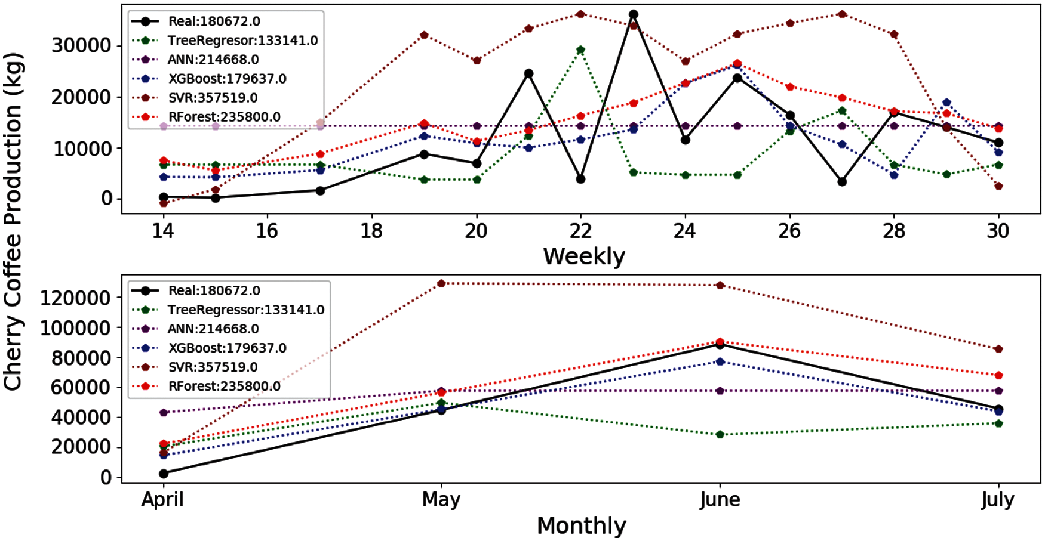
Figure 6: Estimation of coffee production by means of the E-05 experiment. On the x-axis are the months corresponding to the main coffee harvest of the year 2018. And on the y-axis the amount in kg of cherry coffee production
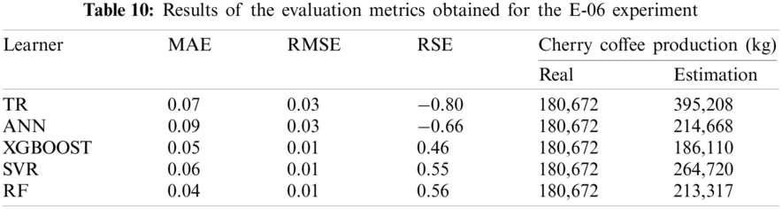
Tab. 10 shows that the results for the evaluation metrics for the E-06 experiment are very similar to the results described for the previous experiments. The XGBOOST and RF algorithms provide the closest estimation to the real coffee production. There is a difference of approximately 1 thousand kilograms for XGBOOST and 55 thousand kilograms for RF. As previously mentioned, the difference between the estimated value and the real one is quite large because the models do not consider variables of coffee beans loss at the harvest stage of the coffee value chain. According to a CENICAFE study [35], the average loss in traditional harvesting is 4.46 coffee beans per tree. However, a coffee crop has approximately from 5 thousand to 10 thousand coffee trees per hectare. In addition, 1 kilogram of mature coffee (cherry) has an average of 555 coffee beans.
Specifically, the case study farm has an average of 4.57 thousand trees per hectare and a total of 38 plots at each hectare. If we calculate the loss of coffee beans per tree, we will obtain 20.40 thousand lost beans per hectare and 775.35 thousand for the complete farm. If we convert this amount to kilograms, we obtain 1.39 thousand kilograms (approximately 1.40 tons) of loss for the complete farm. Finally, it would be also important to consider the loss of coffee beans generated during the transport from the crop to the collection center.
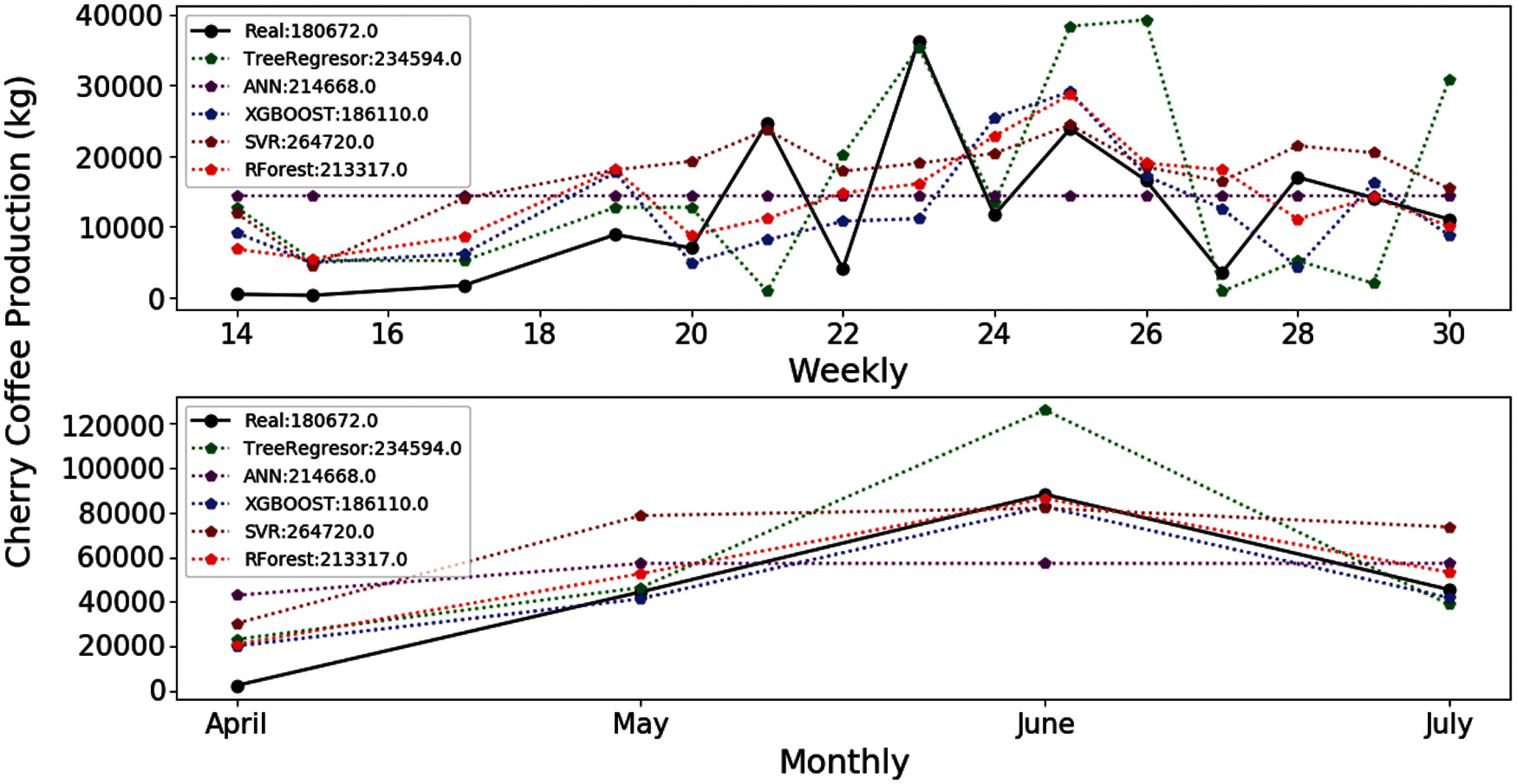
Figure 7: Estimation of coffee production by means of the E-06 experiment. On the x-axis are the months corresponding to the main coffee harvest of the year 2018. And on the y-axis the amount in kg of cherry coffee production
With regard the estimations provided by the different algorithms for the coffee production in the 2018 harvest, they are quite close to the real value (Fig. 7). However, the difference of the best result obtained by the XGBOOST algorithm is higher than the corresponding value obtained for the E-05 experiment. Fig. 7 shows that the XGBOOST and RF algorithms provide satisfactory results also considering that the number of features has decreased considerably.
The 6 experiments described in this section uses different time series configured according to the time scale (monthly and weekly) and different methods of selection of characteristics to estimate the production of cherry coffee. As previously described the best results have been obtained for the E-05 and E-06 experiments given that the target class was normalized to reduce the errors observed in the E-01, E-02, E-03, and E-04 experiments.
We have also analyzed the RMSE and MAE errors in the E-05 and E-06 experiments. The TR, ANN, XGBOOST and RF algorithms provide the lowest values for the RMSE error in the E-05 experiment (Fig. 8a). However, in both experiments the XGBOOST and RF algorithms provide low errors regardless of the feature selection method used in the evaluation process.
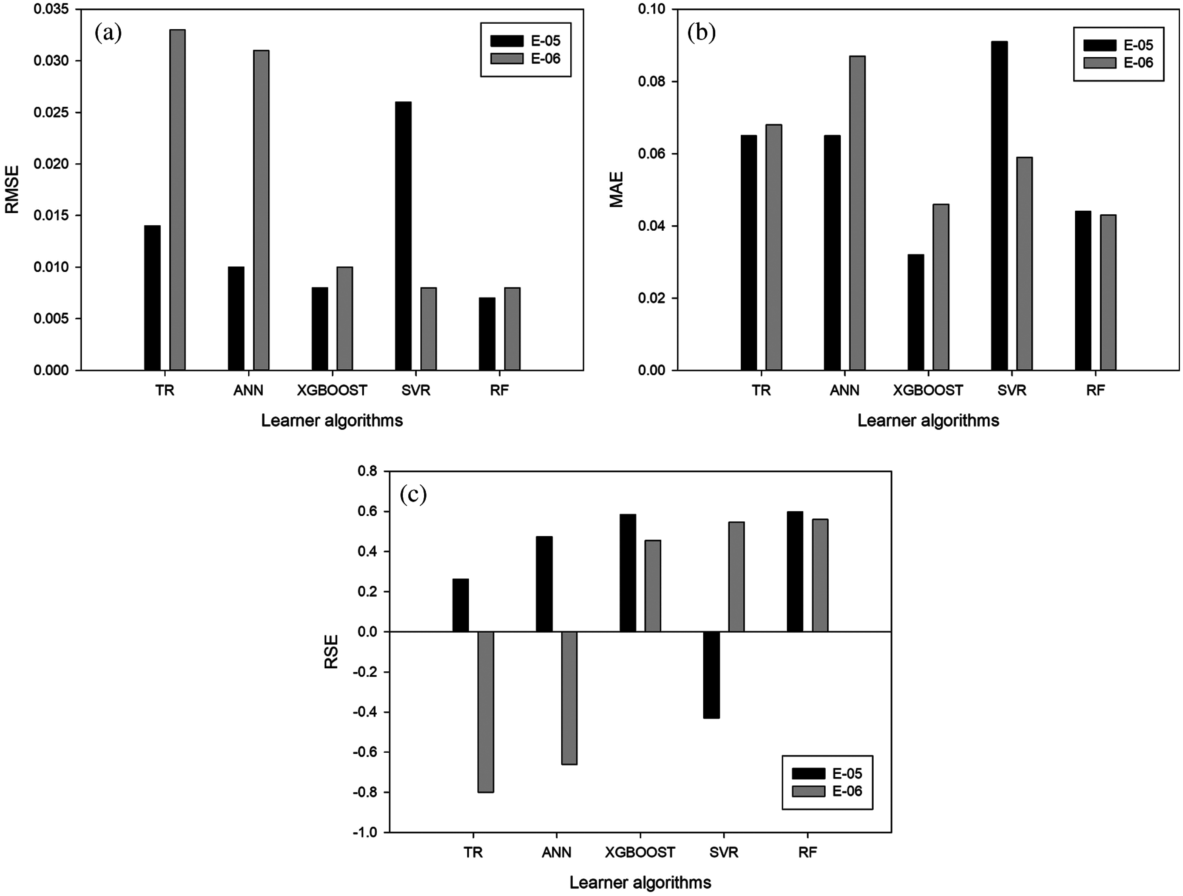
Figure 8: Evaluation measures for the E-05 and E-06 experiments (x-axis: learner algorithms, y-axis: value of the evaluation measure
A similar behavior can be concluded for the MAE error (Fig. 8b). The XGBOOST and RF algorithms provide the lowest values for this measure. The results obtained for the RSE error (Fig. 8c) show that the TR algorithm obtained the lowest errors were for E-05 experiment and the XGBOOST algorithm for the E-06 experiment.
The estimation of cherry coffee production allows coffee growers to plan the required activities and resources, anticipate negotiations, prices and losses of coffee production, and offer a high-quality product considering the number of factors that can affect the production and are not easy to predict. However, as it has been described in the paper, there is a reduced number of research proposals estimating crop yields using statistical methods. This number is even smaller for cherry coffee estimation.
In this paper we have presented a proposal for coffee yield estimation based on the combination of time series and a set of learner models. The detailed evaluation of these models show that the algorithms based on regression trees (XGBOOST, TR and RF) provides very good results for the test dataset collected in real conditions for more than a year. In addition, the model proposed in this research work allows estimating the possibilities of negotiating and complying with the committed delivery terms based on a non-destructive model, unlike the methods currently used by coffee growers.
As a future work, we plan to extend the evaluation considering additional variables of cherry coffee production that are currently being collected and annotated, such as vegetation indices, which can also have a high correlation with crop production. We also want to use alternative deep learning techniques to extend the evaluation.
Funding Statement: We thank to the Telematics Engineering Group (GIT) of the University of Cauca and Tecnicafé for the technical support. In addition, we are grateful to COLCIENCIAS for PhD scholarship granted to PhD. David Camilo Corrales. This work has been also supported by Innovacción-Cauca (SGR-Colombia) under project “Alternativas Innovadoras de Agricultura Inteligente para sistemas productivos agrícolas del departamento del Cauca soportado en entornos de IoT ID 4633 - Convocatoria 04C-2018 Banco de Proyectos Conjuntos UEES - Sostenibilidad”.
Conflicts of Interest: The authors declare that they have no conflicts of interest to report regarding the present study.
1https://www.supracafe.com/ (Last access: March 2021).
2https://www.meteoblue.com (Last access: March 2021).
1. T. Gomiero, “Soil and crop management to save food and enhance food security,” in Saving Food. Production, Supply Chain, Food Waste and Food Consumption, Cambridge, MA, USA: Academic Press, pp. 33–87, 2019. [Google Scholar]
2. M. A. Yost, N. R. Kitchen, K. A. Sudduth, R. E. Massey, E. J. Sadler et al., “A long-term precision agriculture system sustains grain profitability,” Precision Agriculture, vol. 20, pp. 1177–1198, 2020. [Google Scholar]
3. A. A. Gamboa, P. A. Cáceres, H. Lamos, D. A. Zárate and D. E. Puentes, “Predictive model for cocoa yield in santander using supervised machine learning,” in Proc. of STSIVA'19, Bucaramanga, Colombia, pp. 1–5, 2019. [Google Scholar]
4. R. R. d. V. Gonçalves, J. Zullo, T. M. Peron, S. R. M. Evangelista and L. A. S. Romani, “Numerical models to forecast the sugarcane production in regional scale based on time series of NDVI/AVHRR images,” in Proc. of Multi-Temp'15, Annecy, France, pp. 1–4, 2015. [Google Scholar]
5. S. H. Qader, J. Dash and P. M. Atkinson, “Forecasting wheat and barley crop production in arid and semi-arid regions using remotely sensed primary productivity and crop phenology: A case study in Iraq,” Science of the Total Environment, vol. 613–614(C), pp. 250–262, 2017. [Google Scholar]
6. International Coffee Organization, Coffee Market Report January 2019, London, UK, ICO, 2020. [Online]. Available: http://www.ico.org/documents/cy2018-19/cmr-0119-c.pdf. [Google Scholar]
7. Ministry of Agriculture and Rural Development. Bogotá, Colombia, 2020. [Online]. Available: https://sioc.minagricultura.gov.co/Cafe/Documentos/2020-03-31%20Cifras%20Sectoriales.pdf. [Google Scholar]
8. J. R. Rendón-Sáenz, J. Arcila-Pulgarín and E. C. Montoya-Restrepo, “Estimated coffee production based on flowering records,” Cenicafé, vol. 59, no. 3, pp. 238–259, 2008. [Google Scholar]
9. P. Ramos, F. Prieto, C. Oliveros, N. Aleixos, F. Albert et al., “ Measurement of the percentage of maturity in coffee branches using mobile devices and computer vision,” in Proc. of VIII Congreso Ibérico de Agroingeniería, Orihuela, Spain, pp. 917–925, 2015. [Google Scholar]
10. Y. Cai, “Crop yield predictions-high resolution statistical model for intra-season forecasts applied to corn in the US,” in Proc. of AGU Fall Meeting, New Orleans, USA, pp. 1–22, 2017. [Google Scholar]
11. M. Shahhosseini, R. A. Martínez-Feria, G. Hu and S. V. Archontoulis, “Maize yield and nitrate loss prediction with machine learning algorithms,” Environmental Research Letters, vol. 14, no. 12, pp. 1–11, 2019. [Google Scholar]
12. Y. Liu, S. Zhang, H. Yu, Y. Wang, Y. Feng et al., “Straw segmentation algorithm based on modified unet in complex farmland environment,” Computers, Materials & Continua, vol. 66, no. 1, pp. 247–262, 2021. [Google Scholar]
13. W. L. Song, X. Wang, P. Wei, Z. Lu, X. Wang et al., “Blockchain-based flexible double-chain architecture and performance optimization for better sustainability in agriculture,” Computers, Materials & Continua, vol. 68, no. 1, pp. 1429–1446, 2021. [Google Scholar]
14. S. Mishra, D. Mishra and G. H. Santra, “Adaptive boosting of weak regressors for forecasting of crop production considering climatic variability: An empirical assessment,” Journal of King Saud University-Computer and Information Sciences, vol. 32, no. 8, pp. 949–964, 2017. [Google Scholar]
15. P. C. Fernández-Mensaque, F. J. G. Minero, J. Morales and C. Tomas, “Forecasting olive (Olea europaea) crop production by monitoring airborne pollen,” Aerobiologia, vol. 14, no. 2-3, pp. 185–190, 1998. [Google Scholar]
16. B. Garg, S. Aggarwal and J. Sokhal, “Crop yield forecasting using fuzzy logic and regression model,” Computers & Electrical Engineering, vol. 67, pp. 383–403, 2018. [Google Scholar]
17. R. Sujatha and P. Isakki, “A study on crop yield forecasting using classification techniques,” in Proc. of ICCTIDE’16, Kovilpatti, India, pp. 1–4, 2016. [Google Scholar]
18. D. Ramesh, “Analysis of crop yield prediction using data mining techniques,” International Journal of Research in Engineering and Technology, vol. 4, no. 1, pp. 470–473, 2015. [Google Scholar]
19. I. Oliveira, R. L. F. Cunha, B. Silva and M. A. S. Netto, “A scalable machine learning system for Pre-season agriculture yield forecast,” in Proc. of 14th Int. Conf. on e-Science, Amsterdam, Netherlands, pp. 1–8, 2018. [Google Scholar]
20. F. Zhang, B. Wu and C. Liu, “Using time series of SPOT VGT NDVI for crop yield forecasting,” in Proc. of IGARSS'03, Toulouse, France, pp. 386–388, 2003. [Google Scholar]
21. H. Kerdiles, F. Rembold, O. Leo, H. Boogaard and S. Hoek, “CST, a freeware for predicting crop yield from remote sensing or crop model indicators: illustration with RSA and Ethiopia,” in Proc. of Agro-Geoinformatics'17, Fairfax, USA, pp. 1–6, 2017. [Google Scholar]
22. J. Sun, J. Huang, J. Chen and L. Wang, “Grain yield estimating for hubei province using remote sensing data take semilate rice as an example,” in Proc. of ESIAT'09, Washington, USA, pp. 497–500, 2009. [Google Scholar]
23. H. Lee and A. Moon, “Development of yield prediction system based on real-time agricultural meteorological information,” in Proc. of ICACT'14, PyeongChang, South Korea, pp. 1292–1295, 2014. [Google Scholar]
24. X. Xingmei, C. Liying, Z. Jing and S. Fengyan, “Study and application of grain yield forecasting model,” in Proc. of ICCSNT'15, Harbin, China, pp. 652–656, 2015. [Google Scholar]
25. N. Rale, R. Solanki, D. Bein, J. Andro-Vasko and W. Bein, “Prediction of crop cultivation,” in Proc. of CCWC'19, Las Vegas, USA, pp. 227–232, 2019. [Google Scholar]
26. D. G. Mayer, K. A. Chandra and J. R. Burnett, “Improved crop forecasts for the Australian macadamia industry from ensemble models,” Agricultural Systems, vol. 173, pp. 519–523, 2019. [Google Scholar]
27. D. Tedesco-Oliveira, R. Pereira da Silva, W. Maldonado and C. Zerbato, “Convolutional neural networks in predicting cotton yield from images of commercial fields,” Computers and Electronics in Agriculture, vol. 171, pp. 105307, 2020. [Google Scholar]
28. D. C. Corrales, G. Gutiérrez, J. P. Rodríguez, A. Ledezma and J. C. Corrales, “Lack of data: Is it enough estimating the coffee rust with meteorological time series?,” in Proc. of ICCSA'17, Trieste, Italy, pp. 3–16, 2017. [Google Scholar]
29. P. J. Ramos, F. A. Prieto, E. C. Montoya and C. E. Oliveros, “Automatic fruit count on coffee branches using computer vision,” Computers and Electronics in Agriculture, vol. 137, pp. 9–22, 2017. [Google Scholar]
30. J. P. Rodríguez, D. C. Corrales, J. N. Aubertot and J. C. Corrales, “A computer vision system for automatic cherry beans detection on coffee trees,” Pattern Recognition Letters, vol. 136, pp. 142–153, 2020. [Google Scholar]
31. L. Kouadio, R. C. Deo, V. Byrareddy, J. F. Adamowski, S. Mushtaq et al., “Artificial intelligence approach for the prediction of robusta coffee yield using soil fertility properties,” Computers and Electronics in Agriculture, vol. 155, pp. 324–338, 2018. [Google Scholar]
32. D. C. Corrales, A. Ledezma, J. Hoyos, A. Figueroa and J. C. Corrales, “A new dataset for coffee rust detection in Colombian crops base on classifiers,” Sistemas y Telemática, vol. 12, no. 29, pp. 9–23, 2014. [Google Scholar]
33. P. M. Granitto, C. Furlanello, F. Biasioli and F. Gasperi, “Recursive feature elimination with random forest for PTR-mS analysis of agroindustrial products,” Chemometrics and Intelligent Laboratory Systems, vol. 83, no. 2, pp. 83–90, 2006. [Google Scholar]
34. C. J. Willmott and K. Matsuura, “Advantages of the mean absolute error (MAE) over the root mean square error (RMSE) in assessing average model performance,” Climate Research, vol. 30, no. 1, pp. 79–82, 2005. [Google Scholar]
35. F. F. Farfán and P. M. Sánchez, “Planting density of castillo variety coffee in agroforestry systems in the department of santander Colombia,” Cenicafé, vol. 67, no. 1, pp. 55–62, 2016. [Google Scholar]
 | This work is licensed under a Creative Commons Attribution 4.0 International License, which permits unrestricted use, distribution, and reproduction in any medium, provided the original work is properly cited. |