Computers, Materials & Continua DOI:10.32604/cmc.2022.019544
Article

Defocus Blur Segmentation Using Genetic Programming and Adaptive Threshold

Muhammad Tariq Mahmood*

Future Convergence Engineering, School of Computer Science and Engineering, Korea University of Technology and Education, Cheonan, 31253, Byeongcheon-myeon, Korea
*Corresponding Author: Muhammad Tariq Mahmood. Email: tariq@koreatech.ac.kr
Received: 16 April 2021; Accepted: 03 June 2021

Abstract: Detection and classification of the blurred and the non-blurred regions in images is a challenging task due to the limited available information about blur type, scenarios and level of blurriness. In this paper, we propose an effective method for blur detection and segmentation based on transfer learning concept. The proposed method consists of two separate steps. In the first step, genetic programming (GP) model is developed that quantify the amount of blur for each pixel in the image. The GP model method uses the multi-resolution features of the image and it provides an improved blur map. In the second phase, the blur map is segmented into blurred and non-blurred regions by using an adaptive threshold. A model based on support vector machine (SVM) is developed to compute adaptive threshold for the input blur map. The performance of the proposed method is evaluated using two different datasets and compared with various state-of-the-art methods. The comparative analysis reveals that the proposed method performs better against the state-of-the-art techniques.

Keywords: Blur measure; blur segmentation; sharpness measure; genetic programming; support vector machine

1  Introduction

Generally, blur compromises the visual quality of images but sometimes it is induced deliberately to give the aesthetic impression or a graphical effect. Blur can be caused due to the limited depth of field of the lens, wrong focus and/or relative movement of object and camera. Unintentional defocus blur is considered as an undesirable effect because it not only decreases the quality of the image but also leads to the loss of necessary information. Hence automatic blur detection and segmentation play crucial role in many image processing and computer vision applications including forgery detection, image segmentation, object detection and scene classification, medical image processing and video surveillance system [1–3].

In literature, various blur measure operators have been proposed for blur detection and segmentation. A comprehensive study and comparative analysis of a variety of blur measures is presented in [4]. Elder et al. [5] proposed a method to estimate the blur map by calculating first and second order image gradients. Lin et al. [6] suggested the closed-form matting formulation for blur detection and classification, where the regularization term is computed through and local 1D motion of the blurred object and gradient statistics. Zhang et al. [7] suggested the double discrete wavelet transform to get the blur kernels and to process the blurred images. Zhu et al. [8] suggested the local Fourier spectrum to calculate the blur probability for each pixel and then blur map is estimated through solving a constrained energy function. Oliveira et al. [9] proposed a blur estimation technique through Radon-d transform based sinc-like structure of the motion blur kernel and then applied a non-blind deblurring algorithm to restore the blurry and noisy images. Shi et al. [10] proposed a set of blur features in multiple domains. Among them, they observed that the kurtosis varies in blurred and sharp regions. They also suggested the average power spectrum in the frequency domain as an eminent feature for blur detection. Finally, they proposed a multi-scale solution to fuse the features. In another work, Peng et al. [11] suggested the method to measure the pixel blurriness based on the difference between the original and the multi-scale Gaussian-filtered images. The blur map is then utilized to estimate the depth map. Tang et al. [12] proposed a coarse-to-fine techniques for blur map estimation. First, a coarse blur map is calculated by using the log-averaged spectrum of the image and then updated it iteratively to achieve the fine blur map by using the relevant neighbor regions in the local image. Golestaneh et al. [13] exploited the variations in the frequency domain to distinguish blur and non-blur regions in the image. They computed the spatially varying blur by applying multiscale fusion of the high-frequency discrete cosine transform (DCT) coefficients (HiFST). In another work, Takayama et al. [14] have generated the blur map by evaluating the local blur feature ANGHS (amplitude normalized gradient histogram span). Su et al. [15] have suggested the design of a blur metric by observing the connection between image blur and singular value distribution from a single image (SVD). Vu et al. [16] have measured the blur by a block-based algorithm that uses a spectral measure based on the slope of the local magnitude spectrum and a spatial measure based on maximization of local total variation (TV).

Once, blur map is generated, the next step is to segment blur and non-blur regions in the input image. Elder et al. [5] applied local scale control technique. In this technique, they calculate the zero crossing of second and third derivatives in the gradient image and use them for segmentation. Lin et al. [6] calculated the features from local 1D motion of the blurred object and used for regularization to segment the motion and blur from the images. In another method, Zhang et al. [7] computed the Double Discrete Wavelet Transform (DDWT) coefficients-based blur kernels to decouple the blurred regions from the input image. Shi et al. [10] used the graph-cut technique to segment the blurry and non-blurry regions from the blur map. Tang et al. [12] generated super pixels by using simple linear iterative clustering (SLIC) technique by adapting k-means clustering for segmentation. Yi et al. [17] proposed a new monotonic sharpness metric based on local binary patterns that rely on the observation that the non-uniform patterns are more discriminating towards blur regions. The segmentation process is done by using multi-scale alpha maps obtained through the multi-scale blur maps. Whereas, Golestaneh et al. [13] set the fixed threshold empirically, for the segmentation of in-focus and out-of-focus regions in the image. Takayama et al. [14] used Otsu’s method [18] to get the threshold for every map and then it is used to segment the blur and non-blur region of the image. Su et al. [15] extracted the blurred regions of the image by using the singular value-based blur maps. They also applied the fixed threshold to divide the in-focus and out-of-focus regions in the blurred images.

Recently, a large number of deep learning-based methods have been used for blur detection [19–23]. In [22], a convolutional neural network (CNN) based feature learning method automatically obtains the local metric map for defocus blur detection. In [20], fully convolutional network (FCN) model utilizes high-level semantic information to learn image-to-image local blur mapping. In [23], a bottom-top-bottom network (BTBNet) effectively merges high-level semantic information encoded in the bottom-top stream and low-level features encoded in the top-bottom stream. In [21], a bidirectional residual refining network (BR2Net) is proposed that encodes high-level semantic information and low-level spatial details by embedding multiple residual learning and refining modules (RLRMs) into two branches for recurrently combining and refining the residual features. In [19], a layer-output guided strategy based network exploits both high-level and low-level information to simultaneously detect in-focus and out-of-focus pixels.

The performance of the blur segmentation phase very much depends on the capability of blur detection phase. Among various blur detection methods, some perform better than the others in underlying certain conditions. Few most famous and effective methods are using multi-resolution of image in their algorithms. For example, LBP based defocus blur [17] uses three scales with window sizes 11×11, 15×15, and 21×21 to produce three different blur maps and then integrate three maps to get final blur map. Similarly, HiFST [13] uses four scales to generate the initial blur maps and then the final improved blur map is obtained by fusing these initial maps. However, it is very difficult to find an appropriate scale range on which method gives the best results for an arbitrary input image. The performance of a specific blur measure also varies image to image [4]. It means that there is not any single blur measure that can perform consistently for all images taken under varying conditions.

In this paper, we propose a method for blur detection and segmentation based on machine learning approaches. The block diagram of the proposed method is shown in Fig. 1. The proposed method is divided into two phases. In the first phase, a robust GP based blur detector is developed that captures the blur insight on different scales. The multi-scale resolution property is encoded into the blur measure to generate an improved blur map by fusing information at different scales through the GP technique. In the second phase, the blur map is segmented by an adaptive threshold obtained through the SVM model. The performance of the proposed method is evaluated using two different datasets and the results are compared with five state-of-the-art methods. The comparative analysis reveals that the proposed method has performed better against the state-of-the-art methods.

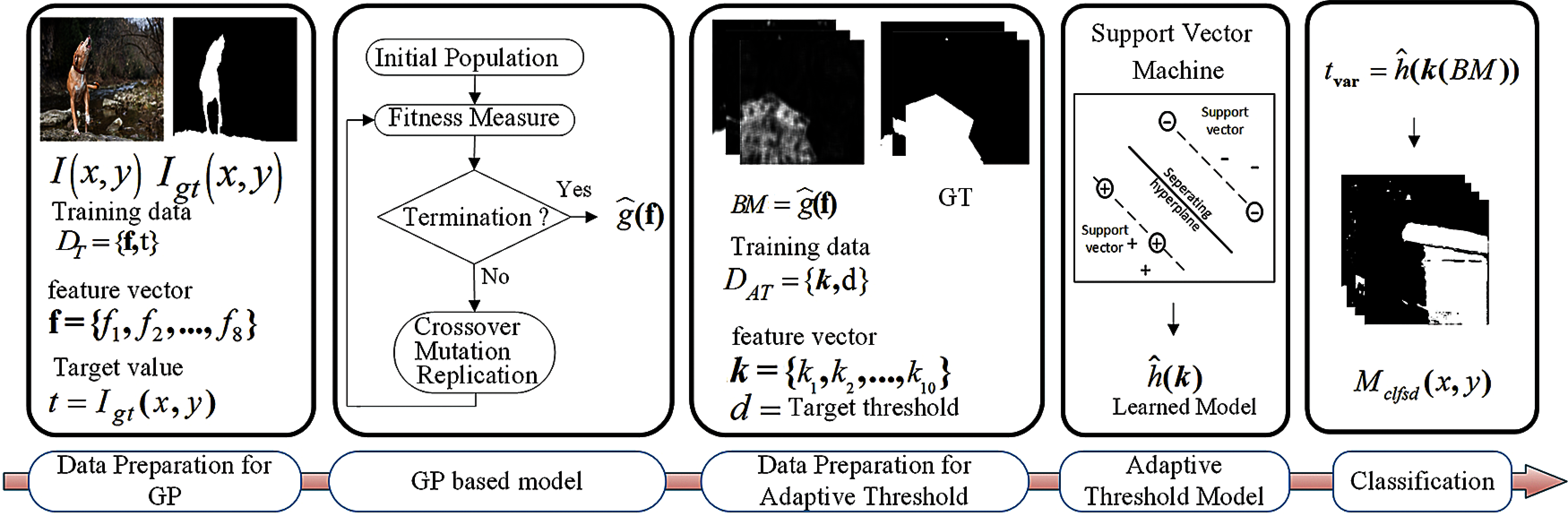
Figure 1: Block diagram for the proposed method for blur detection and segmentation

The rest of the paper is organized as follows. Section 2 discuss the basic rules for the genetic programming techniques. Section 3 presents the details of the proposed method including the details about the development of models. In Section 4, experimental setup, results, and comparative analysis are presented. Finally, Section 5 concludes the study and provides the future directions.

2  Genetic Programming

Multi-Gene Genetic Programming (MGGP) is a variant of GP, which provides model as a linear combination of bias coefficients and multiple genes [24]. Traditional GP, in contrast, gives a model with single gene expression. In MGGP, bias coefficients are used to scale each gene and hence play a vital role to improve the efficacy of the overall model. In MGGP symbolic regression, every prediction of the output variable is a weighted sum of each of the genes plus a bias term. The structure of the multi-gene symbolic regression model is shown in Fig. 2. Mathematically, the prediction of the training data is written as:

y→=b0+b1×G1+...+bM×GM, (1)

where b0 represents the bias term, b1,...,bM are the weights for the genes G1,...,GM and M is the number of total genes. Let Gi be the output vector of the ith tree of size N×1. We define T as gene response matrix of size N×(M+1) as follow.

T=[1G1…GM], (2)

where 1 refers as a (N×1) column of ones used as offset input. Eq. (1) can be written in matrix form as:

y=Tb, (3)

where b represents the weights vector [b0,b1,…,bM]. The optimal weights for initial models participating in multi-gene are determined by applying the least square method.

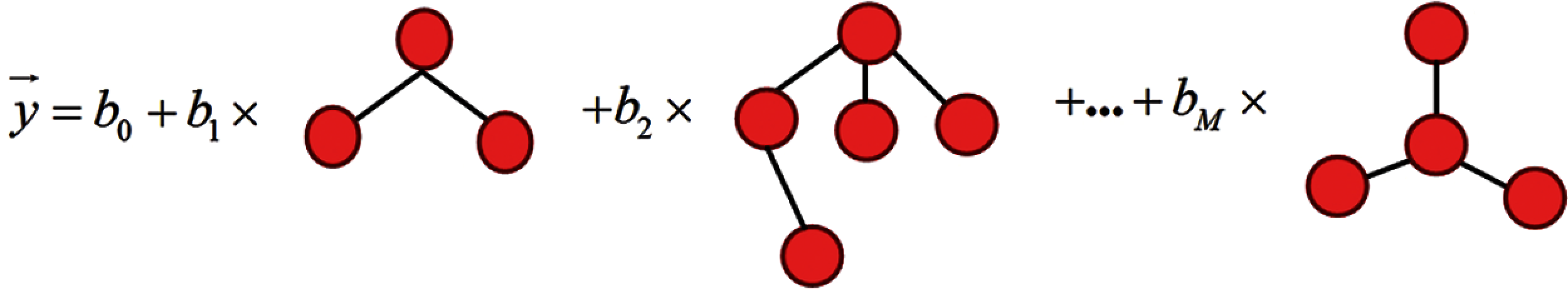
Figure 2: Example of multi-gene regression model

In experiments, individuals in the population have gene restriction between 1 to Gmax and the individual tree depth restriction up to Dmax. These parameters are set to control the complexity of the evolved models. The initial population is created by generating a random GP tree subjected to Gmax and Dmax constraints. During the MGGP run, individuals are probabilistically selected in each generation, and genes in the individual are updated through crossover and mutation operations. In MGGP, the rate based high-level crossover operator is applied which accommodates the exchange of genetic information between the individuals. Rate based high-level crossover operator can be described through the following example. In the crossover between a parent individual consisting of 3 genes labelled as (G1  G2  G3)  and the second parent individual consisting of 5 genes labelled as (G4  G5  G6  G7 G8), the crossover points are randomly selected in each parent, as highlighted in boldface below.

Parent 1: (G1  G2  G3), Parent 2: (G4  G5  G6  G7  G8)

The selected genes are then exchanged to produce two children for the next generation as expressed below.

Offspring 1: (G1  G3  G5  G7) , Offspring 2: (G4  G6  G8  G2)

The sizes of the created offspring are governed by Gmax and Dmax constraints. If the resultant individual contains more genes than the Gmax, additional genes are randomly discarded. In order to achieve higher accuracy of for a model, a robust classifier is required. In this paper, we have used logistic regression as a binary classifier. Logistic regression produces a logistic curve, which is limited to the value 0 and 1 hence used to predicts the probability of an outcome. Mathematically, logistic regression function is defined as:

Pq=11+e−(y) (4)

where Pq is the score for prediction and y is the output for the individual when the training data feature vector DT is fed to the individual as input vector. Fitness function gives the measurement of the accuracy of a particular model, i.e., how well a model can solve the given problem. Fitness function plays a significant role in improving the performance of the system, hence learning the best classifier g^(f). The fitness measure that is used in this paper is area under the receiver operating characteristic (ROC) curve.

3  Proposed Method

In first phase, a GP based model g^(f) is learned to detect the blurriness level of input image pixels which generates a blur map. In the second phase, SVM based classifier h^(k) is developed to predict the best threshold for the blur map. Finally, the segmented map Mclfsd(x,y) is computed by applying the threshold.

3.1 Blur Detection

In this section, GP based blur detection model is developed that generates a blur map for a partially blurred image. This section consists of two parts: (a) preparation of training data for GP, (b) learning best model form GP.

3.1.1 Data Preparation for GP Model

We prepare the training data form a random image I(x,y) and its ground truth image Igt(x,y). Feature vector f=(f1,f2,f3,f4,f5,f6,f7,f8) is constructed with eight features. Where each feature of f is a blur map of LBP and HiFST, calculated on different windows. f1 is generated when the LBP is applied on the image I(x,y) with fixed window size w=11. Similarly f2, f3, f4 are LBP blur map using window size w=15, w=21, w=27 respectively and feature f5 to f8 are the HiFST blur map using window size w=11, w=15, w=21 and w=27 respectively. It is important to note that there are number of possibilities available to construct the feature vector. For example, few more blur measure can be included. Moreover, blur maps can be computed by using different sized windows. Different sized windows are normally used to capture the multi-scale information. In case of blur detection measures, usually a particular sized window is not capable to capture enough information related to diverse types of blurred pixels. Therefore, in the proposed method, features are computed through LBP and HiFST measures using different window sizes. In this way, the GP based method encodes the multi-scale information for blur detection. The target value t for each feature vector is calculated from the ground truth image Igt(x,y). Training data DT is used in GP process to evolve a classifier. Mathematically, training data for GP can be represented as DT={f,t}.

3.1.2 Learning GP Model

In this module, the first phase is to construct an initial population of predefined size. Each individual in the population is constructed with the linear combination of the bias coefficient and set of genes. The bias coefficients are determined by the least square method for each multigene individual. A gene of multigene GP is a tree-based GP model where the terminal nodes are taken from the feature set f, and the entire non-terminal nodes are the arithmetic operators called function set. The terminal set consists of eight nodes f1 to f8, and the function set is made of five nodes. The four nodes are the regular mathematical operators. However, mult3 is the multiplications of three numbers. Times, minus, plus and sqrt has two input arguments each and mult3 has three input arguments, and all operators return single output. All input and output types are floating type values, and therefore, the output of one node can be an input of other nodes. Few important parameters for GP with their values are mentioned in Tab. 1.

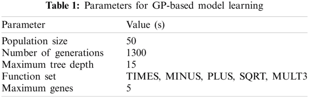
The accuracy of individuals in the population is then evaluated with the fitness function. The best individual is then ranked and selected for the next generation by the selection method. In our experiment, we have used a tournament-based selection method to acquire individuals for the next generation. The crossover and the mutation operator are applied to the selected individuals to produce the population for the next generation. At the end of the evolutionary process the system returns an evolved program g^(f). The performance of the evolved model is then evaluated on the test data. The fitness function used in this paper is AUC, where AUC indicates the area under the curve of receiver operating characteristic (ROC). Once the GP model is developed, we can compute the blur map for every image using bm=g^(f). The GP incorporates multi-scale resolution information in the enhanced blur map BM. Several GP simulations are carried out using the GPTIPS toolbox [24] to achieve an optimal solution.

3.2 Segmentation

In this section, a model for computing adaptive threshold is developed that will be applied on blur map to segment blur and non-blur pixels. This section again consists of two parts: (a) preparation of training data for SVM, (b) learning best model form SVM. Following subsections will explain the preparation of training and testing data, learning of SVM model and model evaluation.

3.2.1 Data Preparation for SVM Model

First, we create a set of useful features. We compute a feature vector k with ten features named as (k1,k2,…,k10). Tab. 2 shows the feature set we have used in our experiment. However, the model accuracy may vary if we choose different features for learning. Mean of all the pixels of an image gives insight about the total brightness. The standard deviation measures the spread of the data about the mean value. Median is a measure of an intensity level of the pixel which separates the high-intensity value pixels and lower intensity value pixels. The covariance of an image is a measure of the directional relationship of pixels. The correlation coefficient calculates the strength of the relationship between the pixels. The entropy measure calculates randomness among the pixels of an image. The skewness of the image contains information probability distribution of the pixels. Negative skew indicates that the bulk of the values lie to the right of the mean, whereas positive skewness indicates that bulk of the values lie to the left of the mean. Kurtosis gives information about the noise and resolution measurement together. The high value of kurtosis values indicates that noise and resolution are low. Contrast contains the distinguishable property of the objects in an image. It is calculated by taking the difference between the maximum and minimum pixel intensity in an image. Energy gives information on directional changes in the intensity of the image.

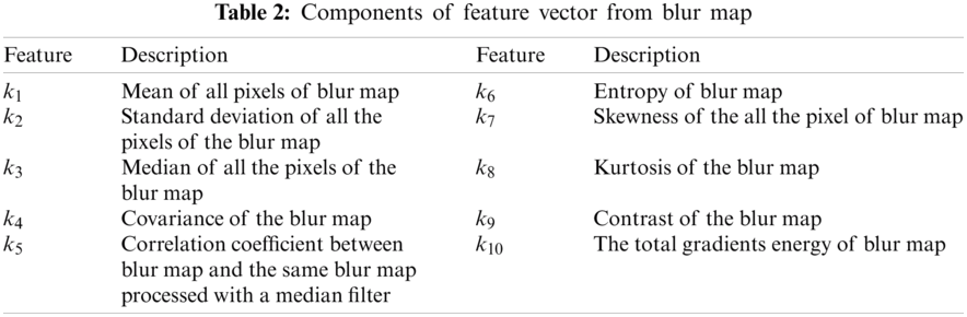
The blur map generated from the GP model is used to generate the features for training data i.e., for each blur map 10×1 dimensional features vector k=(k1,k2,…,k10) is computed. Here, the best threshold for each image is the target value against each feature vector. The best threshold d is computed empirically by segmenting the blur maps and comparing them with the ground truth images. The LBP based blur maps with different window sized were segmented against a set of thresholds. The best threshold d is chosen against the best Accuracy metric. The training data set for learning adaptive threshold is represented as:

DAT={k(i),d(i)}i=1,2,…,N1 (5)

Here, N1 is the sample size of the training data. In our experiment, the total size of the training and testing data is N=N1+N2, where N2 is the sample size of the test data.

3.2.2 Learning SVM Model

Once the training data DAT is ready, a multi-class classifier is being trained using SVM. Multiple binary classifiers can be used to construct a multiclass classifier by decomposing the prediction into multiple binary decisions [25]. To decompose the binary classifier decision into one, we have used ‘onevsall’ coding type. Each class in the class set is individually separable from all the other classes and for each binary learner, one class is taken as positive, and the rest is taken as negative. This design uses all the combinations of positive class for the binary learner. Non-linearity in the features is taken care of by kernel function by transforming nonlinear spaces into linear spaces. All necessary parameters and their appropriate values are listed in Tab. 3. In our experiment, the evolved classifier h^(k) takes the value of feature vector k as an input and classify it into one of the sixteen classes. These sixteen numeric values are the adaptive thresholds for the GP retrieved blur map.

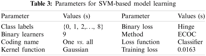
Once the model h^(k) is trained with the training data DAT. The assessment of the learned model is done with test data. The following criteria generate the classified map.

Mclfsd(x,y)={1,if BM≥tvar0,otherwise (6)

To evaluate the performance of the classifier, we compute classification loss (L). It is the weighted sum of misclassified observations and can be represented by the formula:

L=∑i=1N2wiI{tvar(i)−t(i)}, (7)

here, tvar is the threshold predicted by the classifier h^(k), t is the pre-known target value for test data and I{x} is the indicator function. In our experiment, the model accuracy achieved with training data is 98.4%, and with test data, the model performs with the accuracy of 88%.

4  Results and Discussions

4.1 Experimental Setup

In our experiment, we have used two datasets named as dataset A and dataset B. Dataset A [10] is publicly available dataset consists of 704 defocus partially blurred images. This dataset contains a variety of images, covering numerous attributes and scenarios like nature vehicles, humankind, other living, and non-living beings with different magnitude of defocus blur and resolution. Each image of this dataset is provided with a hand-segmented ground truth image-segmenting the blurred and non-blurred regions. Dataset B is a synthetic dataset which consists of 280 out of focus image from the dataset used in [26]. Each image of dataset B is synthetically created by mixing the blur and the focused part of other images of dataset A. However, we have generated the ground truth image by just segmenting the defocus blur and defocus non-blur regions of each image. There is a possibility of biasing of the particular choice of images (i.e., scenario and degree of blurriness) with the blur measure operators because the evaluation performance of the methods may differ for the different input image. Therefore, quantitative analysis on one dataset would not qualify to compare the performance of blur measure operator. There is also the possibility of model over-fitting for g^(f), since the model is trained on the dataset A. In order to mitigate these issues and limitations, we intend to run our quantitative and qualitative analysis on two different datsets A and B. Four quantitative metrics are utilized for the evaluating the performance of the developed classifier. These well-known metrics include Accuracy, Precision, Recall, and F-measure [4,27]. The performance of different methods is evaluated using these three criteria. Accuracy measures the closeness of the measurements to the specific values. It is defined as;

Accuracy=(TN+TP)(TN+TP+FP+FN) (8)

where TP, TN, FP, and FN denote true positive, true negative, false positive, and false negative, respectively. If a pixel is blurred and it is detected as blurred then it is considered as true positive (TP) and if it’s not detected then it is regarded as a false negative (FN). However, if a sharp pixel is detected as a blurred pixel then it is considered as false positive (FP) otherwise it is a true negative (TN). Precision is a measure of the correct positive predictions out of all the positive predictions. It is given by;

Precision=(TP)(TP+FP). (9)

Recall, also called as sensitivity in binary classification, is a measure of ability to retrieve the relevant results. Recall provides the proportion of actual positives that are identified correctly and it is given by the formula;

Recall=(TP)(TP+FN). (10)

F-measure is the harmonic mean of Precision and Recall. It is defined as;

F-measure=(1+β2)(precision∗recall)(β2∗precision+recall). (11)

The recall gets β times more importance as compared to precision. In our experiments, we set β=0.5 that gives more weight to Precision as compared to Recall. As we observed that the proposed method is providing better Recall measures as compared to Precision. In this way, providing smaller weight to Recall is a better choice.

4.2 Comparative Analysis

In order to do comparative analysis, the performance of the proposed method is compared with the five state-of-art methods including (a) LBP based segmentation defocus blur [17], (b) high frequency discrete cosine transform coefficients based method (HiFST) [13], (c) discriminative blur detection features using local Kurtosis (LK) [10], (d) blurred image region detection and classification through singular value decomposition(SVD) [15] and (e) a spectral and spatial sharpness measure based on total variation (TV) [16]. In addition, all experiments were conducted using the computer system with the processor Intel(R) Core (TM) i5-9400F and CPU@2.90 GHz. The operating system Windows 10 was running on the system. Moreover, the software and programs for the proposed method was developed using Matlab 2020a. The Matlab codes provided by the authors for LBP [17]1, HiFST [13]2, LK [10]3, SVD [15]4 and TV [16]5 are used for the comparative analysis. The performance of all the five methods is compared with our proposed method qualitatively and quantitatively by using dataset A and the dataset B. During the computation of blur map, multi-scale resolution windows for LBP and HiFST are same as they mentioned in their respective works and codes. However, for LK, SVD and TV methods, multi-scale windows are not used, so we have used the single window with size w=15×15. Moreover, for LK, SVD and TV methods, the window size w=15×15 is the most appropriate and it provides the best results among others. Binarization is the final step in the blur segmentation process, which is achieved using the threshold computed through the SVM based developed model.

Fig. 3 shows the quantitative comparison of the proposed method and five state-of-art methods including LBP, HiFST, LK, SVD and TV. All methods are applied on each image of two datasets A and B, and four measures: Accuracy, Precision, Recall and F-Measure, are computed. In the Fig. 3, values for the four-performance metrics Accuracy, Precision, Recall and F-Measure are presented. first, for each image in the dataset, the four metrics are computed then the average value for each metric for the whole dataset is computed. The performance average measures for the dataset A are presented in Fig. 3a and the performance average measures for the dataset B are shown in Fig. 3b. From the resultant measures, it is clearly visible that the performance of the proposed method is better than state-of-art methods. Among various methods, KL has provided the poor values for all metrics whereas, LBP and HiFST methods have provided comparable results with respect to the proposed method. On the other hand, SVD and TV methods have provided average performance against all measures. It is important to note that, no image from the dataset B was taken for training process. The results from Fig. 3b shows generalization property of the developed model. It also shows that the prospect of model overfitting is reduced. The noteworthy difference in Recall value for dataset B between the proposed and others methods signifies the robustness of the proposed method.

For qualitative comparison, we evaluate our method on the randomly picked images with different scenarios as well as the different degree of blur from the both datasets A and B. We compare the performance of proposed method with five state-of-art methods five state-of-art methods LBP [17], HiFST [13], LK [10], SVD [15] and TV [16]. First, the blur maps are generated from all methods and the ground truth are also presented for visual comparisons. Fig. 4 compares the visual results for blur maps. The blur maps are presented in the form of grayscale images where the sharp region contain higher intensity pixels and blur regions have low-intensity pixels. It can be observed that the blur maps produced through the proposed method are closer to their ground truths.

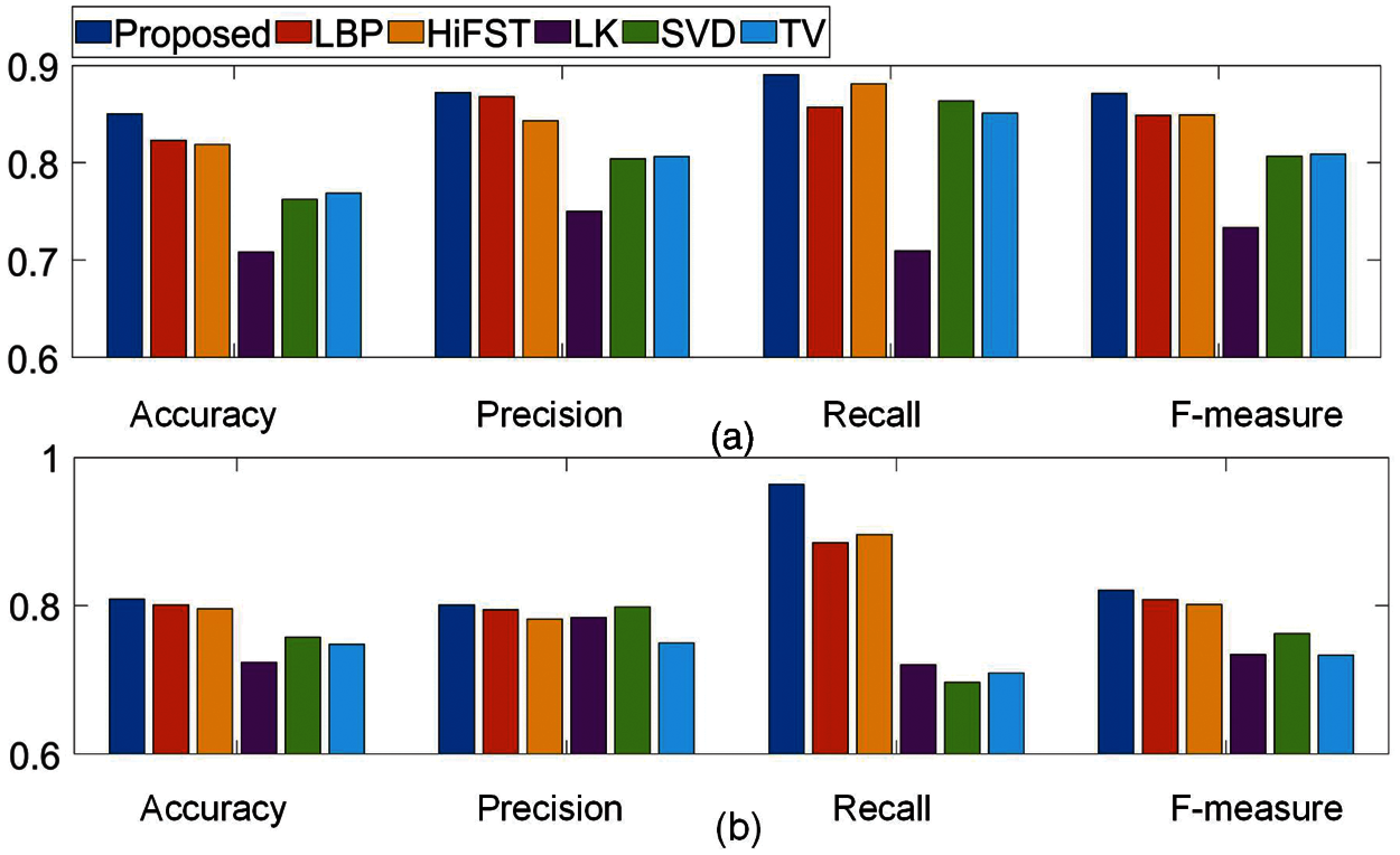
Figure 3: Comparison of the proposed method with state of art methods based on Accuracy, Precision, Recall and F-measure using images of (a) Dataset A with 704 images. (b) Dataset B with 280 images

Whereas, in blur maps produced by KL, SVD and TV methods, degree of blurriness is not correctly estimated The performances from LBP and HiFST methods are comparable with the proposed method. It is clear that the proposed method has ability to estimate degree of blurriness accurately.

The blur maps provided by the all above mentioned methods are segmented using the SVM based classifier and the results are presented in Fig. 5. It can be observed that the proposed method has segmented the blurred and unblurred regions with higher accuracy than other methods, regardless of the blur type and scenarios. Segmented results produced for the LK, SVD and TV methods have inaccuracies due to inaccurate computation of degree of blurriness. Results produced for LBP and HiFST are comparable with the proposed method, however, at few segmented parts inaccuracies are visible. Whereas, the proposed method has provided better segmented maps.

The proposed method has ability of capturing multi-scale information. Here, we analyze the multi-scale performance of the LBP-based segmentation defocus blur [17] at two sets of scale range and compared it with our proposed method. In this experiment, we have chosen scale range S1 = 11, S2 = 15 and S3 = 21 as set-1 and S1 = 23, S2 = 25 and S3 = 27 as set-2. Fig. 6b clearly shows the performance at sets-1 and 2 in their respective classified map and it varies with type of image. We observe that choosing appropriate scale for particular type of image is a challenging task. Fig. 6a shows the blur map and the segmented map of the proposed method. Our algorithm not only resolve the scale issue but also improve the segmentation results significantly.

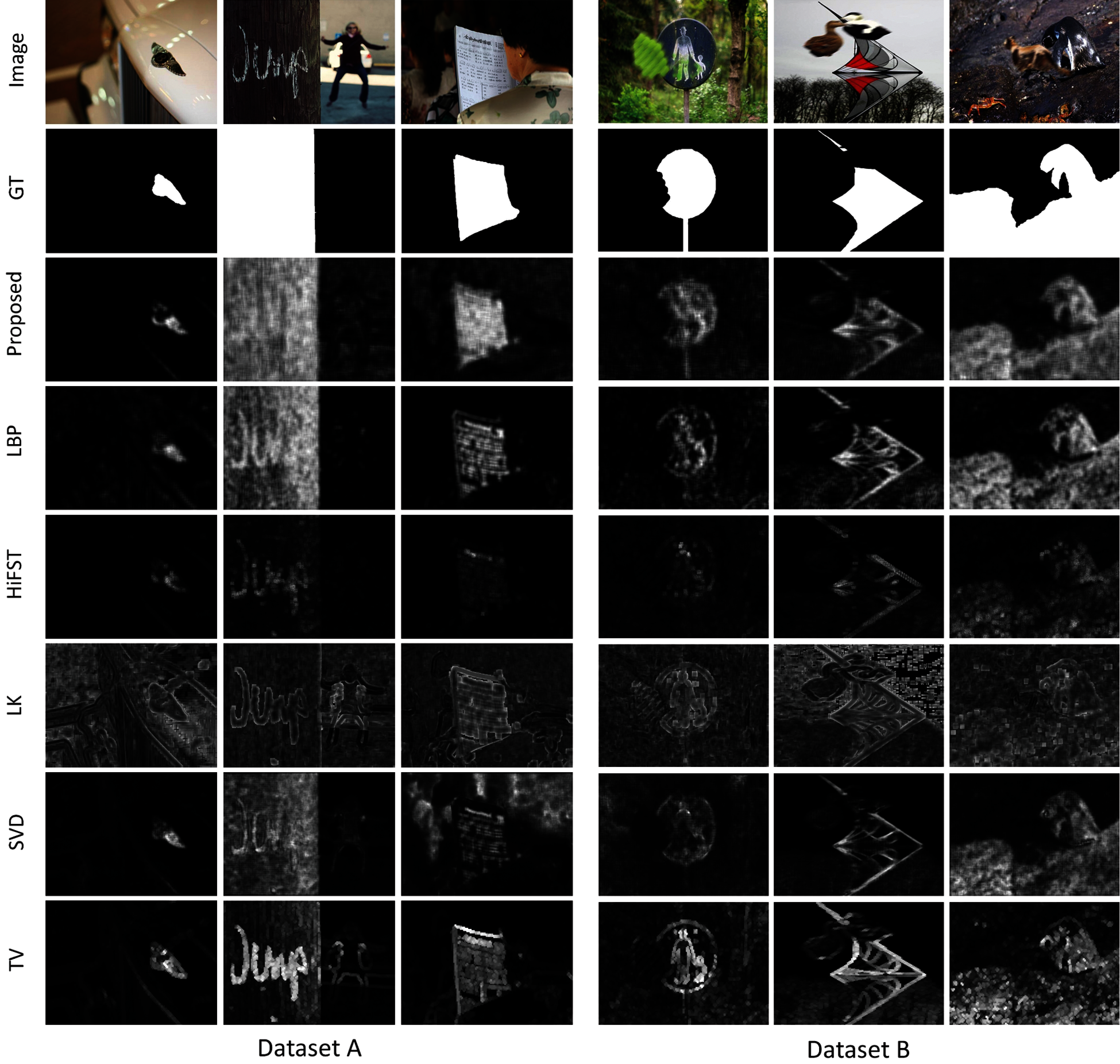
Figure 4: Blur maps computed through for few selected images from dataset A and B. (row1), input images; (row2), ground truths; (row3~row8), blur maps that are computed through the proposed LBP [17], HiFST [13], LK [10], SVD [15] and TV [16] methods, respectively

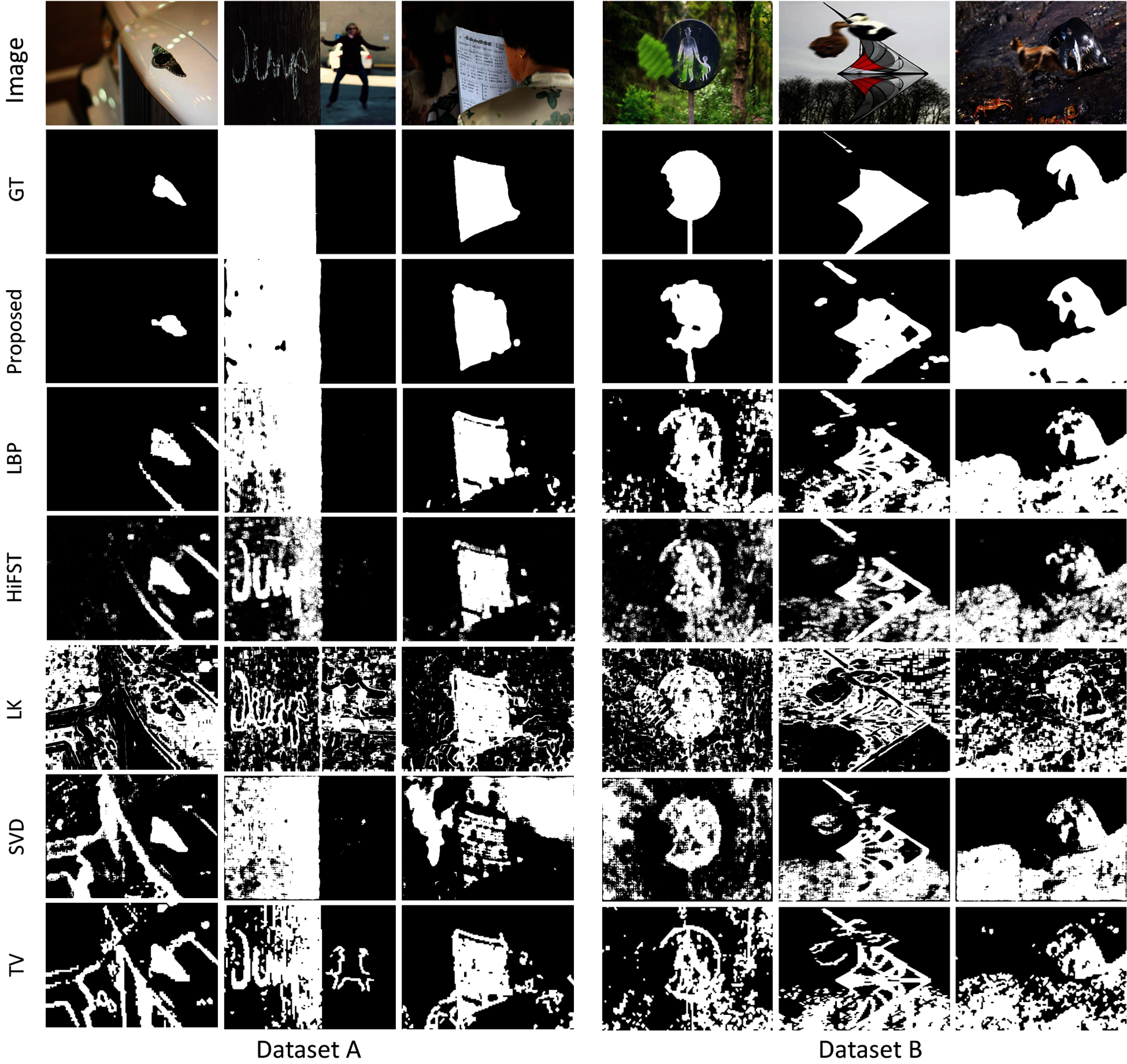
Figure 5: Segmented maps computed through for few selected images from dataset A and B. (row1), input images; (row2), ground truths; (row3~row8), segmented maps that are computed through the proposed LBP [17], HiFST [13], LK [10], SVD [15] and TV [16] methods, respectively

4.3 Limitations

The response of blur measure operator varies on different images, some operator performs better than other on same image due to different blur type, scenario, or level of blurriness. Since proposed method inherit the blur information of two methods HIFST [13] and LBP based defocus blur [17], We could not address the problem of noise propagation in this study. As shown in Fig. 7, on a particular image the performance of HIFST [13] is good and it generates a better blur map, while blur map for LBP [17] contains noise. The noise of low performer method gets propagated during the learning process of GP hence the performance for the proposed method reduced on these images. One more limitation of the proposed method is that it takes more time as compared to the other methods.

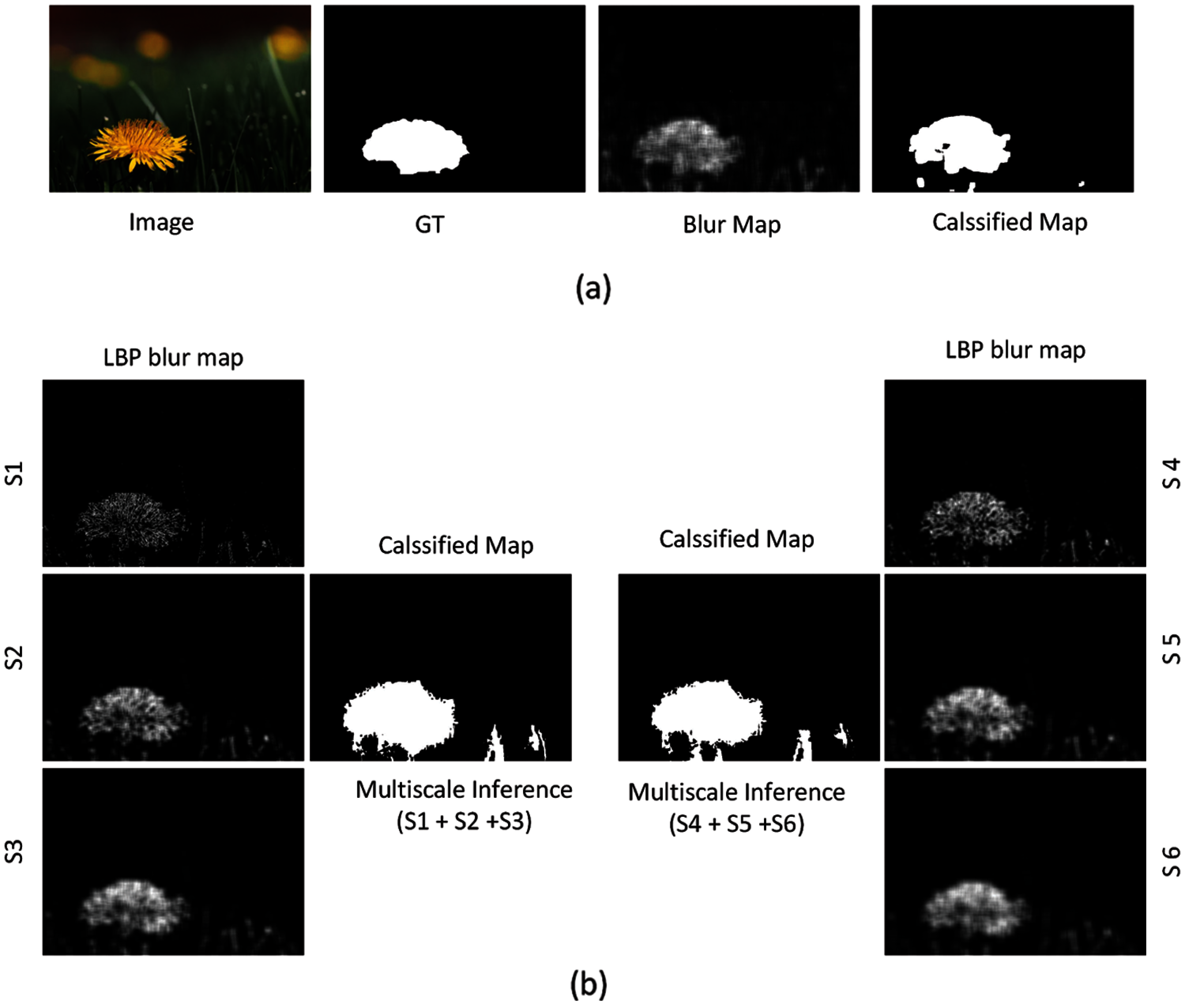
Figure 6: (a) The blur map and the classified map of proposed method (b) LBP blur maps at 2 sets of scale range (S1–S3) and (S4–S6) and their respective classified maps after multi-scale inference

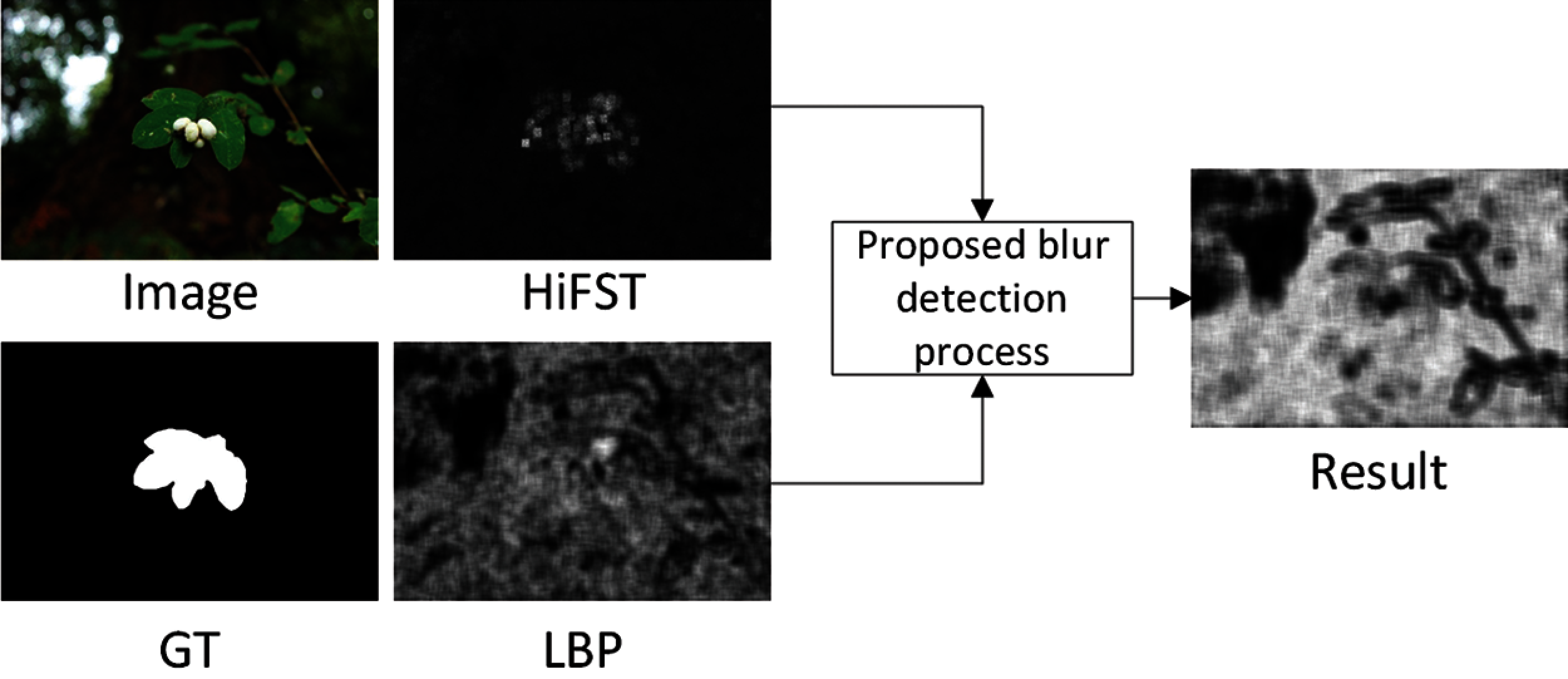
Figure 7: The blur maps of HiFST, LBP and proposed methods for an image which confirms the propagation of noise

5  Conclusion and Future Work

In this article, a robust method for blur detection and segmentation is proposed. Blur detection is achieved by the GP based model, which produces a blur map. For segmentation, first, we trained a model using SVM, which can predict the threshold based on the retrieved blur map features, and then respective thresholds are used to acquire the classified map of the images. We have evaluated the performance of the proposed method in terms of accuracy, precision, Recall, and F-measure using two benchmark datasets. The results show the effectiveness of the proposed method to achieve good performance over a wide range of images, which outperforms the state-of-the-art defocus segmentation methods. In the future, we would like to expand our investigation toward different types of blur. We wish to examine the effectiveness of the proposed approach by learning the combination of motion and defocus blur.

Funding Statement: This work was supported by the BK-21 FOUR program through National Research Foundation of Korea (NRF) under Ministry of Education.

Conflicts of Interest: The authors declare that they have no conflicts of interest to report regarding the present study.

1https://github.com/xinario/defocus_segmentation

2https://github.com/isalirezag/HiFST

3http://www.cse.cuhk.edu.hk/leojia/projects/dblurdetect/index.html

4https://github.com/fled/blur_detection

5http://vision.eng.shizuoka.ac.jp/s3/

This work is licensed under a Creative Commons Attribution 4.0 International License, which permits unrestricted use, distribution, and reproduction in any medium, provided the original work is properly cited.