DOI:10.32604/cmc.2022.020431
| Computers, Materials & Continua DOI:10.32604/cmc.2022.020431 | |
| Article |
Sentiment Analysis on Social Media Using Genetic Algorithm with CNN
Department of Mathematics and Computer Applications, Maulana Azad National Institute of Technology (MANIT), Bhopal, Madhya Pradesh, India
*Corresponding Author: Dharmendra Dangi. Email: dangi28dharmendra06@gmail.com
Received: 24 May 2021; Accepted: 28 July 2021
Abstract: There are various intense forces causing customers to use evaluated data when using social media platforms and microblogging sites. Today, customers throughout the world share their points of view on all kinds of topics through these sources. The massive volume of data created by these customers makes it impossible to analyze such data manually. Therefore, an efficient and intelligent method for evaluating social media data and their divergence needs to be developed. Today, various types of equipment and techniques are available for automatically estimating the classification of sentiments. Sentiment analysis involves determining people's emotions using facial expressions. Sentiment analysis can be performed for any individual based on specific incidents. The present study describes the analysis of an image dataset using CNNs with PCA intended to detect people's sentiments (specifically, whether a person is happy or sad). This process is optimized using a genetic algorithm to get better results. Further, a comparative analysis has been conducted between the different models generated by changing the mutation factor, performing batch normalization, and applying feature reduction using PCA. These steps are carried out across five experiments using the Kaggle dataset. The maximum accuracy obtained is 96.984%, which is associated with the Happy and Sad sentiments.
Keywords: Sentiment analysis; convolutional neural networks; facial expression; genetic algorithm
The continuous increase in social awareness worldwide has been accompanied by an increase in the popularity of social networks such as Twitter. Twitter is one of the most popular social media platforms, where anyone can post tweets to freely express their thoughts and feelings about anything. Low internet fees, inexpensive portable devices, and social responsibility have encouraged people to tweet about various events. For these reasons, Twitter contains a massive amount of data. Tweets cannot exceed 140 characters, meaning that people need to choose their words carefully when expressing their sentiments. They can also augment their posts with images to express their feelings.
Sentiment analysis (or opinion mining) is the assessment of people's opinions or emotions from the text and image data that they provide through, for instance, their tweets. From any given individual, sentiment analysis is based on the specific incident that they are expressing their feelings about [1].
Facial identification comprises three phases: detecting a face, extracting its features, and recognizing the face (Fig. 1). When analyzing facial expressions, much care must be taken to enhance the process of capturing facial expressions that corresponds to human characteristics, as this could provide an effective way for people to interact with facial recognition system.

Figure 1: Three main phases of face recognition
Accurate face recognition can be used for countless uses. The purposes of connecting the regions of a face to various expressions include identifying people; controlling access; recording mobile videos; and improving various applications like video conferencing, forensic applications, interfaces between computers and humans, automatic monitoring, and cosmetology [2].
Many techniques are currently being used to improve face identification methods. Such techniques are highly diverse in terms of what factors they consider—some techniques focus on environmental features, whereas others might deal with direction, appearance, the effect of light, or facial features [3].
Deep learning techniques play an essential role in the classification process. Deep learning is a subcategory of machine learning that deals with the architecture of neural networks [4]. Various deep learning algorithms have been designed to solve many complex real-world problems. Convolutional neural networks (CNNs) are relevant to the present study, as they are used for classification purposes [5]. In this work, CNNs are used to classify images according to the emotions or sentiment. A genetic algorithm (GA) is also used to perform a hyperparameter search to determine which CNN performs the best for the task at hand. The GA's hyperparameters are tuned across five different experiments to attain optimal results.
The remainder of this article is presented as follows: Part 2 discusses the existing sentiment analysis techniques. Part 3 describes the CNN model's integration with the classification of the GA. Part 4 presents and analyzes the simulation results. Part 5 presents the conclusions and suggests future research endeavors.
The concept of face recognition has been widely evaluated since it is relevant to everyone, and the corresponding techniques are easy to use, non-obtrusive, and can be extended if one is willing to accept the extra cost. Many complementary concepts have also been developed throughout the past two centuries through deliberations and research works. Such research shares similarities with research in the fields of the survey, replacement with security (terminals), closed-circuit television (CCTV) control, client validation, human-computer interfaces (HCIs), and intelligent robots, among others.
Several facial recognition techniques have been proposed, including techniques that recognize face architecture. However, no consensus has been reached regarding which design is the best, which is particularly important regarding original surroundings—for instance, determining PCA and ABC by hybridizing them through their office or integrating a family—for enhancement according to demands using a CNN. The determination made at the end of the presentation utilizes the evaluations of false acceptance rate, false rejection rate, and accuracy [6].
Sentiment classification for movie reviews has been utilized through a hybrid classification design. The incorporation of various characteristics and classification techniques, namely the naïve Bayes-genetic algorithm (NB-GA), has been studied, and its accuracy has been assessed. The hybrid NB-GA is more effective than the base classifier, and the GA remains more effective than NB [7].
The polarity of a document is also an essential aspect of text mining. Future engineering with tree kernels has been discussed previously [8]. This technique yields better results than other techniques. The authors who proposed this technique defined two classification models (i.e., two-way and three-way classification). In two-way classification, sentiments are classified as either positive or negative; in three-way classification, sentiments are classified as either positive, negative, or neutral.
The authors considered a tree-based technique for representing tweets in the tree kernel method. The tree kernel-based model achieved the best accuracy and was the best feature-based model. The results showed that this technique performed 4% better than a unigram model.
A hierarchical sentiment analysis approach can also be used for cascaded classification. The authors cascaded three classifications—objective vs. subjective, polar versus non-polar, and positive versus negative—to construct a hierarchical model. This model was compared with a four-way classification (objective, neutral, positive, negative) model. The hierarchical model outperformed the four-way classification model [9].
A domain-specific feature-based model for movie reviews has been developed by [10]. Here, the aspect-based technique is used, which analyzes text movie reviews and assigns a sentiment label to them based on the aspect. Each aspect is then aggregated from multiple reviews, and the sentiment score of a specific movie is determined. The authors used a sentiment WordNet-based technique for feature extraction and to compute document-level sentiment analysis. The results were compared with those obtained using Alchemy API. The feature-based model provided better results than the Alchemy API-based model.
In the short aspect, a wise sentiment result is better than a document-wise result. A sentiment classifier model was previously constructed to classify tweets as positive, negative, or neutral. Specific face recognition techniques have also been involved in the design of holistic techniques based on features, as well as hybrid techniques. These designs comprise principal component analysis (PCA) and two-dimensional principal component analysis (2DPCA), derived from PCA [11].
A model has been developed using PCA, SVM, and the GA for facial recognition. This model presented the highest accuracy (99%) on the face database of the Institute of Chinese Academy of Sciences [12]. An automatic selection of a CNN architecture using a GA has been developed for image classification. An experiment was conducted to estimate the accuracy of the models, with the CNN-GA model achieving the highest accuracy (96.78%) [13].
A genetic-based approach was designed to detect unknown faces via matching with training images. The results yielded by this approach were compared with those provided by PCA and LDA. The GA-based approach outperformed the PCA and LDA approaches [14].
In other work, a hybrid face recognition system was developed by combining CNNs and SVM. The best CNN architectures were obtained with a GA. The last CNN layer was then combined with SVM to optimize the results [15]. Other hybrid designs comprise techniques based on modular Eigenfaces [16]. In addition, researchers have clustered k-means and their derivations for face recognition applications due to their computation efficiency. Autoencoders, including deep autoencoders [17], have been employed broadly and remain complex aspects of face recognition. Although CNN-based techniques require a long training time, they have become the most broadly used techniques for all image processing simulations and facial recognition applications because of their favorable spatial feature consideration capabilities.
Very few works have investigated the use of CNNs and GAs for facial recognition purposes. Therefore, in this work, CNNs are implemented with a GA to improve facial recognition results. Also, a mutation factor change analysis has not yet been done in sentiment analyses in previous works. A detailed description of the methodology is given in the next section.
The main contributions made in this paper are as follows:
• Sentiment analysis is an essential topic of significant relevance in the modern world. This paper describes the use of CNNs with GAs for sentiment analysis.
• This paper serves as a reference for anyone who wants to work on the advancement of CNNs and GAs.
• A comprehensive study of changes in five mutation factors shows how varying the mutation factor in the GA affects a CNN's accuracy.
• The final model provides favorable results for feature reduction using PCA. The results show that dimensionality reduction significantly improves accuracy.
Coding and translating techniques were integrated for the proposed technique. Initially, the data were processed and modified to correlate the dataset with the proposed method.
Fig. 2 provides the architectural design for the proposed sentiment analysis. The primary task was to design a CNN capable of localizing human faces and accurately classifying their facial emotions. Faces were broadly classified as either Happy (positive emotion) or Sad (negative emotion). The main problem faced when training deep learning architectures is the proper selection of hyperparameters, which ultimately governs the overall prediction capabilities of the model. This process of hyperparameter selection was inspired by the real-world natural evaluation process in which a species becomes more powerful and adaptive through a continuous process of mutation and natural selection.
The models were defined such that the hyperparameters represented a unique signature of the models, similar to the DNA of real-world individuals. The complete model training process is outlined as follows:
1. A group of random models with unique hyperparameter combinations was generated as the first-generation models [18].
2. All models were trained with the facial emotion recognition dataset, and each model's accuracy was calculated as its fitness score.
3. Top-performing models from the previous generation were selected. New models were then generated from these top-performing models by combining their hyperparameters.
4. For the newly generated models (i.e., the next generation), the process is repeated (starting from step 2) until the desired model is obtained.

Figure 2: Overview of the architectural design
The dataset was taken from a Kaggle facial expression recognition challenge [19]. The dataset contained cropped 48x48 greyscale face images with the corresponding emotion collected from multiple sources, including social media, movies, and the Internet. The overall dataset was divided into seven emotion categories (Angry, Disgust, Fear, Happy, Sad, Surprised, and Neutral). The Happy and Sad subsets (See Fig. 3) of the dataset were the most suitable for the current task.

Figure 3: Sample of image dataset (Happy and Sad)
The Happy and Sad subclasses of the dataset were used as positive and negative sentiments, respectively, during training. Six thousand samples were randomly selected from the dataset for each class. These samples were eventually used for the purposes of training and validation. The sampled dataset was split into 80% training and 20% validation subsets by random selection. The images’ pixel values were also normalized within the range of 0–1 and divided by 255, thus making the data input into the model more generalizable. This process, in turn, improved the processes of learning and regulating the model weights [20].
The overall CNN architecture was divided into three blocks, with each block containing two convolution layers and one MaxPooling layer. These blocks were then followed by a Flattened layer and a Dense layer, which were finally linked with two nodes of the Dense layer, each representing a class from our dataset (i.e., positive and negative). The basic block used in the model architecture is depicted below in Fig. 4.

Figure 4: CNN model architecture block
The convolution layers used in the blocks use “same padding” to ensure that the input and output image sizes of these convolution layers are the same. As a result, the output of each block is just half of the input size (e.g., 48x48xc1 → block → 24x24xc2). In this way, we ensured a proper input size was available for the next block regardless of the filter size and filter counts used in the block.
The output image dimensions for any given padding value p are derived with the given formula seen in Eq. (1) [21].
where
n → input image dimension, p → padding to be used, f → filter size in the same dimension,
s → filter stride value for the same direction
When the above formula is implemented on both input image dimensions (i.e., height and width), the output image size is calculated using Eq. (2).
where
subscript 1 → values corresponding to the first dimension of the images (height),
subscript 2 → values corresponding to the second dimension of the images (width)
In cases where the padding is the same for both dimensions, the required image output size should be the same as that of the input size, as shown in Eq. (3).
Therefore, to keep the input image and output image size equal for each convolution layer, the padding value needs to be updated dynamically according to the corresponding filter size, input and output image size, and filter stride value.
The padding value required to implement the same padding can be derived using Eq. (4) [22].
Since the Convolution2D layers used the same padding as described above, the input image and the output filter map size were the same for both Convolution2D layers in the block. Finally, these layers were followed by the MaxPooling layer, which concluded the output of the layer.
Using the output image dimension formula, we can define the output image size for the blocks, as the input image size and output image size were the same for the Convolution2D layers. Also, the input image size for the MaxPooling layer was the same as that of the input image size of the block.
For the MaxPooling layer, filter size → (2x2), filter stride → (2x2), padding → 0.
Therefore, the output image dimension formula is derived as Eq. (5) [23].
Using a MaxPooling layer with the above configurations reduces the input image size to half its original size by combining the output results of the Convolution2D layers with the same padding, followed by the MaxPooling layer. The resulting output image size can be calculated using Eq. (6).
where
n1 → input image height, n2 → input image width, nc → number of channels in the input image,
fs → filter size for the block, fc → filter count for the block
The above equation clarifies that the block output image's dimensions are halved in both dimensions (height and width) with each block's operation on the input image. Also, the channel count is interchangeable with the block's total filter count value.
Only the filter size and filter count are needed for the blocks to function completely. Therefore, a block can be uniquely defined based solely on the values of these two parameters. The same square filter size and filter count are used in the Convolution2D layers. The MaxPooling2D layer's kernel/filter size is fixed to 2x2.
Since the CNN architecture comprises three blocks (see Fig. 5), a CNN model's complete architecture can be defined if the filter sizes and filter counts of each block are known. These filter sizes and filter counts represent the genes of the CNN model or individual.

Figure 5: Model gene visualization
The filter sizes and filter counts depicted in the above figure are represented with the help of two Python lists—one for filter sizes and another for filter counts. The list's length is equivalent to that of several blocks (three blocks in the present case). Based on the above figure, the model gene can be represented as follows:
((Filter_size_1, Filter_size_2, Filter_size_3), (Filter_count_1, Filter_count_2, Filter_count_3))
3.4 Genetic Algorithm Approach
The primary task of the GA approach is to find the best filter size and filter count combination or gene (collectively). This combination is that which produces the best results for the problem at hand when used to generate a CNN.
Steps
1. Random initialization of population
• Random filter size and filter count values are determined from the given selection range.
• The population size is maintained at 10 individuals.
2. Training of individuals
• Individuals are trained with the given training dataset.
• TensorFlow's early stopping callback is also employed to stop training if the validation loss has not decreased over the last 10 epochs.
3. Calculating individuals’ fitness
• Each individual's validation accuracy is considered as its fitness.
4. Selecting the top-performing individuals based on their fitness
• The top four individuals are selected based on their fitness scores.
5. Repopulating the population with the selected individuals
6. Repeating the process from step 2 to step 5 until an individual with the desired fitness is obtained
This section describes the simulation analysis performed for face sentiment recognition using the proposed CNN-GA.
A complete simulation has been carried out for the proposed CNN-GA using a Python tool in which the architecture has been considered. The experiment has been done using a PC with Windows 10 OS, 4GB RAM, and Intel I5 processor.
The proposed CNN-GA is simulated based on the true negative rate (TNR), true positive rate (TPR), and accuracy. All of this is evaluated using the classification report of the best model. The ROC-AUC curve for the best model is also shown. The classification report describes the accuracy, recall, precision, F1 score, and support. These values can be calculated with a confusion matrix [24]. The formulas used to calculate accuracy, recall, precision, and F1 score are as follows:
Accuracy: Accuracy resolves the proximity for detection by the classifier, which is determined by Eq. (7).
A true positive (TP) occurs when a value is predicted to be positive and is later confirmed to be positive in an AI model. A false positive (FP) occurs when a value is predicted to be negative but is later shown to be positive in an AI model. A true negative (TN) occurs when a negative value is predicted and later confirmed by an AI model. A false negative (FN) occurs when a value is predicted to be positive but is later shown to be negative in an AI model.
Mean generation fitness: This parameter provides an overview of the overall performance of all individuals in a specified generation during GA training as shown in Eq. (8).
Pseudo Code for the CNN-GA:

Pseudo Code 1 determines the overall approach followed by the GA to find the best-performing hyperparameter configuration. The code starts with the initialization of an initial population of randomly generated individuals with constrained parameters. After this, all individuals are trained, and their capabilities and performance are verified. Next, a new generation of individuals is formed via the crossover and mutation of the best-performing individuals from the previous generation. During this process, the best-performing individual is defined as that whose gene or hyperparameter configuration is the best for the problem at hand. This individual's track is kept.
The architecture is simulated with different hyperparameters to obtain better results. Five different experiments are conducted to improve the accuracy of the model. The models are compiled using the ‘adam’ optimizer. As techniques ranging from basic to advanced are considered in this work to increase the model's accuracy, it is understandable that the models evolved across generations of the GA-based approach.
Experiment 1: All default values
The configurations used for this initial baseline experiment for the GA training are:
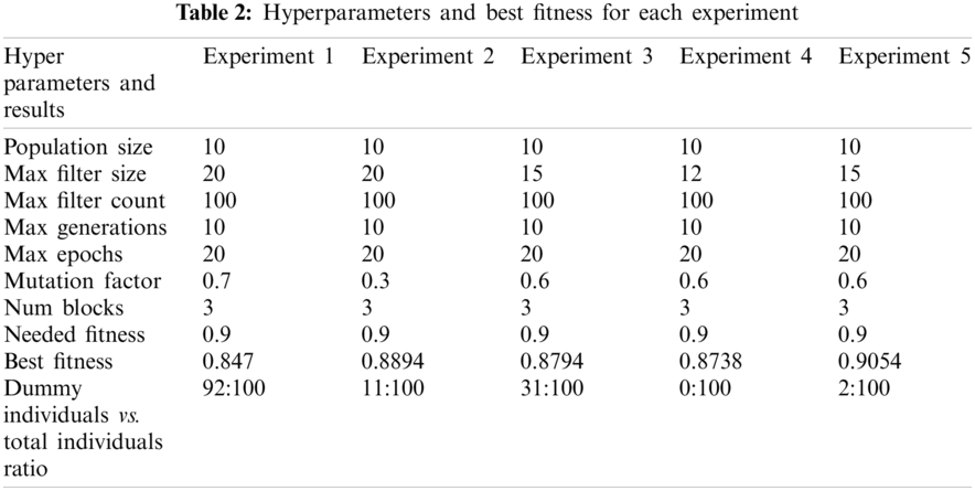
population_size = 10, max_filter_size = 20, max_filter_count = 100, max_generations = 10, max_epochs = 20, mutation_factor = 0.7, num_blocks = 3, needed_fitness = 0.9
Results obtained:
The best model had a fitness value of 0.847 with gene ((5, 1, 1), (72, 83, 101)). The maximum mean generation fitness obtained was 0.6437. The ratio of dummy individuals to total individuals was 92:100.
Observations:
Since the problem starts as a two-class classification problem, the individuals always predict a single class—by doing this, they can easily achieve 50% accuracy. We refer to these individuals as dummy individuals. Due to the high mutation factor (i.e., 70%), variance was high among the repopulated individuals. Therefore, a significant part of the population was unable to properly receive their parents’ genes.
As a result, all models had approximately 50% accuracy (dummy individuals). Since the maximum filter size was 20, the block's input size was sometimes smaller than the filter size. Because those blocks served as identity layers (i.e., they merely sped up the transfer of input into output without applying filters), they contributed nothing to individuals’ fitness. Only 8% of individuals learned properly; all others were dummy individuals. The result is weak child generations.
Experiment 2: Mutation factor 0.3
In this experiment, we tried to solve the problem presented in Experiment 1 (i.e., the high number of dummy individuals). This was a problem because dummy individuals cannot specialize well in the classification problem at hand. This problem was resolved by reducing the mutation factor from 0.7 to 0.3 (i.e., 30% of the individuals in the new generation were mutated).
Configuration used for the GA:
population_size = 10, max_filter_size = 20, max_filter_count = 100, max_generations = 10, max_epochs = 20, mutation_factor = 0.3, # earlier = 0.7, num_blocks = 3, needed_fitness = 0.9
Results obtained:
The best model in this experiment had a fitness value of 0.8894 with gene ((2, 6, 6), (93, 29, 16)). The maximum mean generation fitness obtained was 0.8626. The ratio of dummy individuals to total individuals was 11:100.
Observations:
By reducing the mutation factor, we obtained a high number of learner individuals that could efficiently classify emotions. After further observations of the results, we saw that many individuals remained the same as we moved on to higher generations due to the low mutation factor. The whole process depended substantially on the first generation's genes, which did not help the population acquire different genes (which, in turn, could have led to better results).
Experiment 3: Mutation factor 0.6
Reducing the mutation factor limited the GA's ability to generate high-performing mutated individuals. Therefore, the properties of generated individuals resembled those of randomly generated individuals. Therefore, in this experiment, a mutation factor of 0.6 was selected (i.e., 60% of the generated individuals were mutated).
The configurations used in this experiment are as follows:
population_size = 10, max_filter_size = 15, max_filter_count = 100, max_generations = 10, max_epochs = 20, mutation_factor = 0.6, # default = 0.7, num_blocks = 3, needed_fitness = 0.9
Results:
The best model in this experiment had a fitness value of 0.8794 with gene ((3, 2, 6), (101, 64, 16)). The maximum mean generation fitness obtained was 0.7983. The ratio of dummy individuals to learner individuals was 31:100.
Observations:
These configurations provide better results in terms of the learner and dummy individual counts. In this case, 69% of the individuals were capable of learning and classifying our dataset—however, we still failed to achieve the desired fitness. The problem associated with having redundant blocks serve as identity layers was also reduced when the max_filter_size was decreased. While investigating the reason underlying lower accuracy, we looked into the training and validation losses of the individuals, which showed high overfitting in the individuals toward the training data.
Experiment 4: Mutation factor 0.6 and batch normalization
As observed in Experiment 3, we achieved a reasonable dummy-to-learner ratio, and the problem of blocks working as identity layers was also reduced. Even so, the individuals exhibited overfitting, resulting in high training accuracy (approx. 96–98%) and low validation accuracy (80–83%). In order to overcome this problem, we added batch normalization and dropout layers in the blocks (see Fig. 6). At this point, the blocks were as follows:

Figure 6: Modified CNN model architecture block with additional regularization layers
Configurations used for the GA in this experiment:
population_size = 10, max_filter_size = 12, # default = 20, max_filter_count = 100, max_generations = 10, max_epochs = 20, mutation_factor = 0.6, # earlier = 0.7, num_blocks = 3, needed_fitness = 0.9
Results obtained:
The best model in this experiment had a fitness value of 0.8738 with gene ((2, 3, 6), (93, 38, 16)). The maximum mean generation fitness obtained was 0.8536. The ratio of dummy individuals to total individuals was 0:100.
Observations:
After adding batch normalization, all of our models became learners, which is a strong sign that the population generates better next-generation individuals, thus indicating an upward trend in mean generation fitness. However, even upon observing the training accuracy and validation accuracy, the individuals were still overfitting. When the best individual from this experiment was tested with real-world images, it could not classify the sentiments correctly, showing poor generalization of the individuals.
Experiment 5: Using the Happy and Sad subsets
After a thorough investigation, it was found that the overfitting was due to an insufficient Angry subset of the original dataset. Experiment 4 was performed (with the same configurations imposed on the Happy and Sad subsets of the original dataset) to overcome this. This yielded very promising results, as the best individual's fitness was 0.9038.
The following configurations were applied to the GA:
population_size = 10, max_filter_size = 15, # default = 20, max_filter_count = 100, max_generations = 10, max_epochs = 20, mutation_factor = 0.6, # default = 0.7, num_blocks = 3, needed_fitness = 0.9
Results:
The best model in this experiment had a fitness value of 0.9054 with gene ((3, 4, 16), (101, 98, 101)). The maximum mean generation fitness obtained was 0.8687. The ratio of dummy individuals to total individuals was 2:100.
Observations:
• The overfitting problem was reduced by shifting to the Happy and Sad subsets of the dataset.
• The model generalized well to real-world images.
Generalized results:
• Fig. 7 below depicts the mean generation fitness values of all the experiments in a single graph. As can be seen, the overall results and learning abilities increased with each experiment when we used optimized GA configurations.

Figure 7: Mean generation fitness with all mutation factors
4.3.1 Model's Hyperparameter Space Visualization with PCA
Hyperparameter optimization is a very time-consuming process because the overall parameter space to be traversed (i.e., the space that mirrors the probability space used for probability calculations) is so vast that it is impossible to test all possible hyperparameter combinations. Assuming that a hypothetical model has x hyperparameters that govern the model's overall performance, the number of possible combinations of hyperparameters is the total number of possible discrete values multiplied by the number of parameters.
In this study, the possible hyperparameter combinations for the provided parameter ranges are depicted in Tab. 1.

Due to the massive number of possible combinations, it is crucial to employ an appropriate hyperparameter optimization technique that efficiently finds the best possible combination from among all possible combinations in a way that satisfies the problem at hand.
The grid search and random search methods cover most of the parameter space following a structured approach. Still, these approaches sometimes miss the best-performing parameter region due to a lack of information about the model's fitness in different regions. Our GA approach overcomes this problem by traversing the parameter space while considering the model's fitness. In other words, the GA approach focuses on regions with high model fitness (see Fig. 8).

Figure 8: Assuming a two-hyperparameter model, the traditional hyperparameter optimization techniques (i.e., grid search and random search) traverse the hyperparameter space as depicted in the figure. Each point in the figure represents a unique hyperparameter combination formed by the intersection of specific hyperparameter values from the corresponding axis, thus resembling a unique model configuration selected using the respective approach
The first generations of the GA are randomly initialized. As a result, hyperparameter combinations were selected randomly from the overall hyperparameter space, as in the random search approach. The following generation's individuals were then generated based on the performance of the models of previous generations, which helped the individuals traverse the parameter space in a more performance-centric manner.
The GA's performance in the hyperparameter search within this parameter space can be better understood if all models are depicted in a single graph. In such a graph, each point represents a model's unique gene or set of hyperparameters (similarly to the depictions of the grid search and random search methods presented in the above figure). Considering three blocks per model with one filter size and one filter count per block, a model can be uniquely represented as the combination of the six hyperparameters considered in this research. Because six hyperparameters (or, to put it another way, six-dimensional values) are required to represent a single model, it is impossible to visualize such values on a 2D plane.

Figure 9: The reduction of six-dimensional data to two-dimensional data (named Reduced Hyperparameter 1 and Reduced Hyperparameter 2) with the help of PCA for the sake of visualizing the model's hyperparameter combinations on a 2D plot
PCA was performed based on these six hyperparameters to transform the six-dimensional data into two-dimensional data. Thus, the same model can be represented using just two values instead of six while retaining most of the important information (Fig. 9).
Based on the obtained two-dimensional values, all models obtained by the GA hyperparameter search are plotted into the 2D plot presented in Fig. 10. The figure provides a visualization of how the GA can traverse the parameter space.

Figure 10: A plot of all hyperparameter combinations generated and analyzed by the GA after being reduced into two-dimensional data. Hyperparameter combinations generated in the respective experiments are depicted with corresponding colors
Final Model Training with Best Model Genes:
Considering all experiments together, the best-performing model was that with genes ((3, 4, 16), (33, 98, 101)) in Experiment 5, as it had a fitness value of 0.9054. When the model with these gene values was trained individually for significant epochs, it achieved 96.984% accuracy when compared to the best model. The ROC curve, precision-recall curve, and classification report for this best model are as follows:
Confusion Matrix:
The accuracy can be calculated using Eq. (7) from the normalized confusion matrix (Fig. 11) as follows:
Accuracy = 96.984%

Figure 11: Confusion matrix
Precision-Recall Curve and ROC Curve:
The precision-recall curve corresponding to the result is given in Fig. 12. The ROC-AUC curve reflecting the accuracy is depicted in Fig. 13.

Figure 12: Precision-recall curve

Figure 13: ROC curve with AUC
Tab. 2 summarizes the hyperparameters and experiments.
4.3.2 Comparison with Previous Works
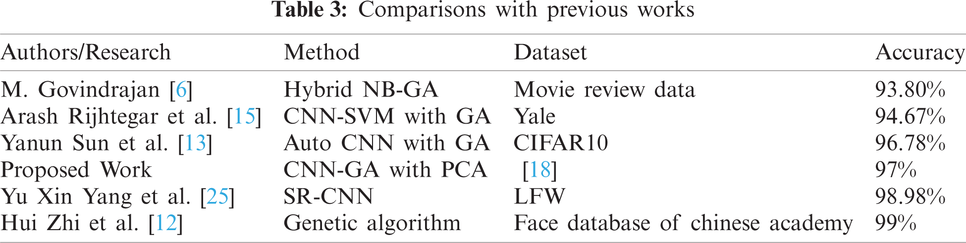
A comparison shows that where your work exists. A result of 96.984% is obtained for a binary classification of Happy and Sad images from a set of experiments where the GA hyperparameters are changed to find the best CNN architecture. The results of experiments should be compared only when they have the same setup and are performed in the same environment. Nevertheless, comparisons between the current results and those of other works are presented in Tab. 3.
This paper developed an algorithm in which CNNs are combined with a GA, which can generalize well to different CNN architectures. This results in a complete autonomous training method that finds the best combinations of hyperparameter configurations for the problem at hand. The research objective was successfully achieved by designing a generalized GA-based CNN hyperparameter search strategy.
The proposed approach was examined using a Kaggle face sentiment dataset [18]. A comparison with the top-performing approaches in the field revealed that this approach achieves up to 96.984% accuracy. Moreover, the proposed approach is automatic, making it easy to use, even for users without comprehensive knowledge of CNNs or GAs.
The scope of advancement of this work is described as follows:
• In this study, the GA was applied only to filter sizes and filter counts for three blocks. The experimental protocol can be performed on more hyperparameters in the future.
• Better algorithms can be employed for the crossover and mutation of new individuals.
• A better initialization technique of first-generation individuals could reduce overall training time.
• A comprehensive discussion can be held regarding variations among crossover methods in the GA so that sentiments can be analyzed more accurately.
• Sentiment analyses using different GAs (e.g., particle swarm optimization, honey bee optimization, ant colony optimization) can be evaluated.
• Genetic evolutionary techniques, hill-climbing, simulated annealing, and Gaussian adaptation could perhaps achieve better results through optimization.
The most notable limitations of this work are as follows:
• The GA-based hyperparameter search is quite a slow process when large parameter spaces are involved.
• The improper initialization of first-generation individuals could lead to inefficient individuals.
• The minimum and maximum limits for the parameter space play a vital role in convergence speed.
Funding Statement: The authors received no specific funding for this study.
Conflicts of Interest: The authors declare that they have no conflicts of interest to report regarding the present study.
1. R. Jongeling, P. Sarkar, S. Datta and A. Serebrenik, “On negative results when using sentiment analysis tools for software engineering research,” Empirical Software Engineering, vol. 22, no. 5, pp. 2543–2584, 2017. [Google Scholar]
2. A. Insaf, A. Ouahabi, A. Benzaoui and A. T. Ahmed, “Past, present, and future of face recognition: A review,” Electronics, vol. 9, no. 8, pp. 1188, 2020. [Google Scholar]
3. W. Wójcik, K. Gromaszek and M. Junisbekov, “Face recognition: Issues, methods and alternative applications,” In Face Recognition-Semisupervised Classification, Subspace Projection and Evaluation Methods, S. Ramakrishnan (Eds.London, UK: IntechOpen, pp. 7–28, 2016. [Google Scholar]
4. W. Zang, Z. Wang, D. Jiang, X. Liu and Z. Jiang, “Classification of MRI brain images using DNA genetic algorithms optimized tsallis entropy and support vector machine,” Entropy, vol. 20, no. 12, pp. 964, 2018. [Google Scholar]
5. D. Jeff, Y. Jia, O. Vinyals, J. Hoffman, N. Zhang et al., “Decaf: A deep convolutional activation feature for generic visual recognition,” in Int. Conf. on Machine Learning, PMLR, pp. 647–655, 2014. [Google Scholar]
6. M. Govindarajan, “Sentiment analysis of movie reviews using hybrid method of Naive Bayes and genetic algorithm,” International Journal of Advanced Computer Research, vol. 3, no. 4, pp. 139, 2013. [Google Scholar]
7. A. Agarwal, B. Xie, I. Vovsha, O. Rambow and R. Passonneau, “Sentiment analysis of twitter data,” in Proc. LSM, Portland, Oregon, pp. 30–38, 2011. [Google Scholar]
8. G. Aaryan, V. Dengre, H. A. Kheruwala and M. Shah, “Comprehensive review of text-mining applications in finance,” Financial Innovation, vol. 6, no. 1, pp. 1–25, 2020. [Google Scholar]
9. D. R. Kawade and K. S. Oza, “Sentiment analysis: Machine learning approach,” International Journal of Engineering and Technology (IJET), vol. 9, no. 3, pp. 2183–2186, 2017. [Google Scholar]
10. J. Tao and X. Fang, “Toward multi-label sentiment analysis: A transfer learning based approach,” Journal of Big Data, vol. 7, no. 1, pp. 1–26, 2020. [Google Scholar]
11. K. Zhang, Y. Huang, Y. Du and L. Wang, “Facial expression recognition based on deep evolutional spatial-temporal networks,” IEEE Transactions on Image Processing, vol. 26, no. 9, pp. 4193–4203, 2017. [Google Scholar]
12. H. Zhi and S. Liu, “Face recognition based on genetic algorithm,” Journal of Visual Communication and Image Representation, vol. 58, no. 18, pp. 495–502, 2018. [Google Scholar]
13. Y. Sun, B. Xue, M. Zhang, G. G. Yen and J. Lv, “Automatically designing CNN architectures using the genetic algorithm for image classification,” IEEE Transactions on Cybernetics, vol. 50, no. 9, pp. 3840–3854, 2020. [Google Scholar]
14. P. Sukhija, S. Behal and P. Singh, “Face recognition system using genetic algorithm,” Procedia Computer Science, vol. 85, pp. 410–417, 2016. [Google Scholar]
15. R. Arash, M. Pooyan and M. T. M. Shalmani, “Genetic algorithm-optimized structure of convolutional neural network for face recognition applications,” IET Computer Vision, vol. 10, no. 6, pp. 559–566, 2016. [Google Scholar]
16. H. Y. Leung, L. M. Cheng and X. Y. Li, “A FPGA implementation of facial feature extraction,” Journal of Real-Time Image Processing, vol. 10, no. 1, pp. 135–149, 2015. [Google Scholar]
17. E. Gumus, N. Kilic, A. Sertbas and O. N. Ucan, “Evaluation of face recognition techniques using PCA, wavelets and SVM,” Expert Systems with Applications, vol. 37, no. 9, pp. 6404–6408, 2010. [Google Scholar]
18. M. Feurer and F. Hutter, “Hyperparameter optimization,” In Hutter F., Kotthoff L., Vanschoren J. (eds) In Automated Machine Learning, Springer, Cham, pp. 3–33, 2019. [Google Scholar]
19. Facial Expression Kaggle Dataset, “Challenges in representation learning: Facial expression recognition challenge,” 2013. [Online]. Available: https://www.kaggle.com/c/challenges-in-representation-learning-facial-expression-recognition-challenge/data. [Google Scholar]
20. J. Gu, Z. Wang, J. Kuen, L. Ma, A. Shahroudy et al., “Recent advances in convolutional neural networks,” Pattern Recognition, vol. 77, pp. 354–377, 2018. [Google Scholar]
21. M. Hashemi, “Enlarging smaller images before inputting into convolutional neural network: Zero-padding vs. interpolation,” Journal of Big Data, vol. 6, no. 1, pp. 1–13, 2019. [Google Scholar]
22. M. Puttagunta and S. Ravi, “Medical image analysis based on deep learning approach,” Multimedia Tools and Applications, vol. 80, pp. 1–34, 2021. [Google Scholar]
23. M. Alam, J. F. Wang, C. Guangpei, L. V. Yunrong and Y. Chen, “Convolutional neural network for the semantic segmentation of remote sensing images,” Mobile Networks and Applications, vol. 26, no. 1, pp. 200–215, 2021. [Google Scholar]
24. G. Chaubey, D. Bisen, S. Arjaria and V. Yadav, “Thyroid disease prediction using machine learning approaches,” National Academy Science Letters, vol. 44, pp. 1–6, 2020. [Google Scholar]
25. Y. X. Yang, C. Wen, K. Xie, F. Q. Wen, G. Q. Sheng et al., “Face recognition using the SR-CNN model,” Sensors, vol. 18, no. 12, pp. 4237, 2018. [Google Scholar]
 | This work is licensed under a Creative Commons Attribution 4.0 International License, which permits unrestricted use, distribution, and reproduction in any medium, provided the original work is properly cited. |