DOI:10.32604/cmc.2022.020455
| Computers, Materials & Continua DOI:10.32604/cmc.2022.020455 | |
| Article |
Deep Stacked Ensemble Learning Model for COVID-19 Classification
1Department of Information Technology, VNRVJIET, Hyderabad, 500090, India
2Department of Computer Science and Engineering, VNRVJIET, Hyderabad, 500090, India
3LBEF Campus, Kathmandu, 44600, Nepal
4Statistics and Operations Research Department, College of Science, King Saud University, Riyadh, 11451, Kingdom of Saudi Arabia
5Operations Research Department, Faculty of Graduate Studies for Statistical Research, Cairo University, Giza, 12613, Egypt
6Wireless Intelligent Networks Center (WINC), School of Engineering and Applied Sciences, Nile University, Giza, 12588, Egypt
*Corresponding Author: Ali Wagdy Mohamed. Email: aliwagdy@gmail.com
Received: 25 May 2021; Accepted: 01 August 2021
Abstract: COVID-19 is a growing problem worldwide with a high mortality rate. As a result, the World Health Organization (WHO) declared it a pandemic. In order to limit the spread of the disease, a fast and accurate diagnosis is required. A reverse transcript polymerase chain reaction (RT-PCR) test is often used to detect the disease. However, since this test is time-consuming, a chest computed tomography (CT) or plain chest X-ray (CXR) is sometimes indicated. The value of automated diagnosis is that it saves time and money by minimizing human effort. Three significant contributions are made by our research. Its initial purpose is to use the essential finetuning methodology to test the action and efficiency of a variety of vision models, ranging from Inception to Neural Architecture Search (NAS) networks. Second, by plotting class activation maps (CAMs) for individual networks and assessing classification efficiency with AUC-ROC curves, the behavior of these models is visually analyzed. Finally, stacked ensembles techniques were used to provide greater generalization by combining finetuned models with six ensemble neural networks. Using stacked ensembles, the generalization of the models improved. Furthermore, the ensemble model created by combining all of the finetuned networks obtained a state-of-the-art COVID-19 accuracy detection score of 99.17%. The precision and recall rates were 99.99% and 89.79%, respectively, highlighting the robustness of stacked ensembles. The proposed ensemble approach performed well in the classification of the COVID-19 lesions on CXR according to the experimental results.
Keywords: COVID-19 classification; class activation maps (CAMs); visualization; finetuning; stacked ensembles; automated diagnosis; deep learning
The coronavirus (COVID-19) was first noted in December 2019 in Wuhan City (Hubei, China). The viral infection quickly spread worldwide, eventually causing a global pandemic. Following a detailed study of its biological properties, the virus was found to be of zoonotic origin and consists of a single-stranded ribonucleic acid (RNA) genome with a strong capsid. Based on this survey, it was concluded that the virus belongs to the coronaviridae family and was subsequently named 2019-novel coronavirus (nCOV). A person infected with 2019-nCoV may have no symptoms or develop mild symptoms, including sore throat, dry cough, and fever. If the human body hosts the 2019-nCoV for a long period, the virus can cause severe respiratory illness and, in the worst case, it can lead to death. There are four stages that are used to assess the virus's virulence in the human body. During the first four days of the infection, the patient is often asymptomatic. The second stage is the progressive stage which generally occurs between the fifth and eighth day following the infection, whereby the patient may develop mild symptoms. Stage three is known as the peak stage, which occurs between nine and thirteen days. The final stage is the absorption stage, whereby the load of the virus exponentially increases [1]. These observations were reported with clinical experimentation in Fig. 1 [2].

Figure 1: An upsurge in the number of cases and death rate from January to July 2020 is depicted. The infection and death rate increased by approximately 105 within six months
Due to the rapid surge in cases, healthcare systems are finding it increasingly difficult to cope with the demand and to provide timely vaccination [3]. This problem is being further exasperated by the shortage of medical supplies globally. In order to reduce the burden on healthcare systems, several preventive measures such as social distancing, proper sanitization, the mandatory wearing of masks in public places, and lockdowns have been implemented worldwide to reduce the spread. Despite the implementation of all these measures, the mortality rate from the disease is still high in various countries. According to the Chinese National Health Commission (NHC), as of February 4th, 2020, the mortality rate from the disease was 2.1% in China and 0.2% outside of China. The mode of spread of the virus in asymptomatic cases remains controversial [4,5]. In order to identify COVID-19 in an asymptomatic person, precise and proper diagnostic tests are required. The diagnostic tests are typically performed by collecting samples from the individual patient for testing in a laboratory or at a point of care testing center [6]. Manual testing is time consumes and labor-intensive. Therefore this method is not suitable to obtain a fast diagnosis during a pandemic. Computed tomography (CT) and chest X-ray (CXR) can be used to detect and assess the severity of the lung damage caused by the viral infection. However, a radiologist needs to analyze these images manually, which is time-consuming. Artificial intelligence (AI) can be used to develop algorithms to automatically assess the lung damage caused by the virus [7,2]. The findings for the COVID-19 infection in CXR or chest CT vary from person to person. However, two common hallmark imaging features observed in infected patients were bilateral and peripheral ground-glass opacities and peripheral lesions with a rounded morphology [2]. These distinct features facilitate the use of machine vision learning models to automatically detect COVID-19 lesions on either CXR or CT images. However, traditional methods do not preserve the contextual information of CT scan images. In view of this, this study aimed to develop a robust diagnostic model for COVID-19 detection on CXR images. The objectives of this study were to:
• analyze the behavior and performance of various vision models ranging from inception to Neural Architecture Search (NAS) networks followed by appropriate model finetuning,
• visually assess the behavior of these models by plotting class activation maps (CAMs) for individual networks,
• determine the classification performance of the model by calculating the area under the curve (AUC) of a receiver operator curve (ROC),
• improve the generalization of the model by combining the finetuned model deep learning with the shocked model (stacked ensembles technique).
Numerous studies evaluated the use of deep learning methods for the automatic detection, classification, feature extraction, and segmentation for COVID-19 diagnosis from CXR and CT images. This study discusses the relevant applications of pre-trained deep neural networks that prompt the key aspects to impact COVID-19 detection and classification. Fan et al. [8] proposed the use of the deep learning network Inf-Net for the segmentation of COVID-19 lesions on transverse CT scan images. This network architecture utilized Res2Net as a backbone and obtained a dice score of 0.682. A similar semi-Inf-Net model attained a higher dice score of 0.739. Oh et al. [9] implemented two different approaches, global patch matching, and local patch matching, for segmentation and classification. Their method used ResNet-18 as the backbone to classify four different types of lung infections similar to that of COVID-19. Their algorithm obtained an accuracy score of 88.9% and specificity of 0.946 on randomly cropped patches using a local approach. Rahimzadeh et al. [10] constructed the 8-phase training concatenating Xception and ResNet-50 architectures. In each phase, samples were trained using a proper stratification to overcome class imbalance for 100 epochs. This model attained an overall accuracy score of 91.4% by five-fold cross-validation. Ozturk et al. [11] proposed a Dark-CovidNet model for binary and tri-class classification of CXR images infected with COVID-19. This model was trained by constructing a deep neural architecture with a series of convolutional layers and max-pooling layers. This method attained accuracy scores of 98.3% for the binary classification and 87.2% for the tri-class classification on five-fold cross-validation. Apostolopoulos et al. [12] applied transfer learning using diverse pre-trained architectures on two different datasets for the classification of COVID-19 CXR images. Their transfer learning methodology attained an accuracy score of 98.75% using VGG-19 pre-trained weights for binary classification and an accuracy of 94.7% for the MobileNet-V2 CXR images classification consisting of three classes. Li et al. [13] proposed the CovNet network by training a deep learning model with ResNet-50 as a backbone for sharing weights and attained an accuracy of 96%. Khan et al. [14] designed the CoroNet-architecture with Xception as an underlying weight-sharing model. This model achieved an accuracy score of 99% through binary classification, 95% when using three non-identical classes (one class belonging to COVID-19), and 89.6% for four variant classes following a four-fold cross-validation framework. Wang et al. [15] proposed the use of COPEL-Net to segment COVID-19 pneumonia lesions from CT images. The novel dice loss combined with a MAEloss for generalization was used to reduce noise and minimize the foreground and background imbalance for the segmentation task. This diagnostic frame obtained a dice score of 80.72 ± 9.96. Most COVID-19 classification and segmentation on CXR and CT images described in the literature are based on deep neural networks. The advantage of deep neural networks is that they provide a versatile weight-sharing mechanism, thus improving the performance of the algorithm. Therefore, this study aimed to develop a robust diagnostic COVID-19 model using CXR images. The objectives of the study were to:
• examine the behavior and efficiency of different deep learning vision models ranging from Inception to NAS networks, using the proper finetuning procedure,
• visually assess the behavior of these models by plotting class activation maps (CAMs) for individual networks,
• determine the classification performance of the model by calculating the area under the curve (AUC) of a receiver operator curve (ROC),
• improve the generalization of the model by combining the finetuned model deep learning with the shocked model (stacked ensembles technique).
A total of 2905 CXRs were obtained from various databases, including the Italian Society of Medical Radiology (SIRM), ScienceDirect, The New England Journal of Medicine (NEJM), Radiological Society of North America (RSNA), Radiopaedia, Springer, Wiley, Medrxiv, and other sources Fig. 2. The complete source list of the COVID-19 CXR image samples is available in the metadata file [16]. These images were reviewed by an expert radiologist. Eight percent (n = 219) of these images were from patients infected with COVID-19%, 46% (n = 1341) of the images were from healthy persons, and the rest of the images were from patients suffering from either bacterial or viral pneumonia (n = 1345) [16]. The data was then divided into 75% training (Dtrain) and 25% testing datasets (Dtest). Due to the small number of CXRs with COVID-19 lesions, stratified random sampling was used to ensure that all three diagnoses were equally represented in both training and testing datasets and hence minimize the risk of introducing class imbalance in the data distribution.

Figure 2: Pie chart illustrating the CXR sources
3.2 Convolutional Neural Networks for Feature Extraction
Convolutional neural networks (CNNs) are increasingly being used in computer vision to detect, classify, localize, and segment normal and pathological features from medical images [17]. The use of CNN increased widely following its application in large-scale image recognition challenges (ILSVRC-2010). In this challenge, AlexNet [18] made use of a deep CNN and resulted in the lowest detection error rate. This motivated researchers to make use of this technology to develop multidisciplinary high-end applications [19]. The CNN architecture can be modified significantly by manipulating the width, depth, and channels (activation-maps) to further improve the performance of the model with appropriate generalizations. Furthermore, the model's performance can be further improved through the manipulation of parametric weight sharing from one network to another network. This technique facilitates the feature extraction procedure in most networks, eventually reducing the computational and training cost [20,21]. Following the successful implementation of AlexNet, numerous other CNNs were developed. In the following section, the advantages and limitations of each CNN are discussed.
The Inception architecture is designed with a novel ideology module. This network architecture is trained by widening layers to increase the depth of the network depth with a few computational parameters. There are two versions of the architecture, including a naive and a dimensionality-reduced. The Inception module consists of three levels. The bottom levels of inception feed into four different layers stacked by width. The intermediate layers extract spatial information individually and correlate with each layer. The top layer concatenates all the intermediate layer's feature maps to maintain a hierarchy of features to improve the perceived performance of the network [22].
After Inception, VGG networks were developed by a sequential convolutional layer with a pooling layer. The sequential depth of the models ranged from 11 to 19 layers. The appropriate use of the max-pooling layers in 16 and 19 layered VGG-Nets is essential for spatial sub-sampling and the extraction of generic features at the rearmost layers. VGG-Nets use small receptive fields of 5x5 and 3x3 to capture small features, eventually improving their detection precision accurately. The generalizability of the model for highly correlated inputs can be further improved by finetuning the learning application schedules to decrease the learning rate [23].
The Res-Nets were developed to address the problem of vanishing gradients by imparting identity mapping in large-scale networks. They reformulated deep layers by aggregating learned activations from a prior layer to form a residual connection. This residual learning minimizes the problem of degrading and exploding gradients in the deeper networks. These residual connections help in addressing learned activations from preceding layers, maintaining a constant information flow throughout the network, and eventually reduce the computational cost [24–26].
This network was inspired by the Inception network modules and identity mappings from ResNets. This method integrates dimensionality-reduced Inception modules with sequential residual connections hence increasing the learning capability of the network while reducing its computational cost. This provides better generalization ability when compared to various versions of the ResNet and Inception Networks [25].
This network was proposed to compete with the Inception network to reduce its flaws. The simultaneous mapping of spatial and cross-channel correlations guides allows for improved learning with small receptive fields and improves perceptive ability. The depth-wise separable convolutional layers enhance the learning through detailed feature extraction. These networks are computationally less expensive and perform better than the Inception network [27].
These densely connected CNNs are motivated by the residual connection of Res-Nets and imposed long-chained residual connections to form dense blocks. In Dense-Nets, for N layers, there are N(N+1)/2 connections (including residual connections) that enhance the network's capability for extracting detailed features while reducing image degradation. The sequential dense and transition blocks provide a collection of knowledge, and a bottleneck receptive field of 3x3, eventually improving its computational efficiency. The finetuning of larger weights improves generalization in deeper networks with a depth ranging from 121 to 201 layers [28].
Mobile-Nets were designed for mobile applications under a constrained environment. The main advantage of this network is the combination of inverted residual layers with linear bottlenecks. The constructed deep-network accrues a low-dimensional input, which eventually expands by elevating dimensional space. These elevated features are filtered via depth-wise separable CNNs and are further projected back onto a low-dimensional space using linear CNNs. This contribution reduces the need to access the main mobile application memory, thus providing faster executions through the use of a cache-memory [29].
Nas-Nets make use of convolution cells by learning from distinct classification tasks. The design of this network is based on a reduced depth-wise stacking of normal cells, hence providing an appropriate search space by decoupling a sophisticated architectural design. This adaptability of Nas-Nets enables it to perform well even on mobile applications. The computational cost is significantly reduced, and its performance can be improved by enhancing the depth [30].
4 Deep Stacked Ensemble Method
This deep-stacked ensemble method was evaluated by classifying COVID-19 database inputs into a tri-class and a binary class, as shown in Fig. 3.

Figure 3: The complete methodology of the deep-stacked ensemble method
Various samples were first considered and pre-processed to a specific resolution of 224×224×3 of the COVID-19 dataset. These pre-processed images were then fed into a variety of deep networks that use different paradigms to extract features from latent dimensions. The extracted feature vectors are then evaluated, and the two best-performing models are selected to form a stacked ensemble. The COVID-19 class is given more weight in this ensemble, which was assessed by classifying the feedback into a tri-class and a binary class.
4.1 Finetuning of Neural Networks
Deep learning algorithms can accurately detect pathology from bio-medical imaging to human-level precision. The CNNs provide numerous advantages for feature detection in medical imaging. There are two methods that can be used to design neural architectures for medical imaging. The first method involves designing a novel architecture by overhauling loops in existing architectures by training it end-to-end. The second method involves model finetuning by either transferring the weights of a pre-trained model (transfer of weights) or by retraining an existing pre-trained architecture.
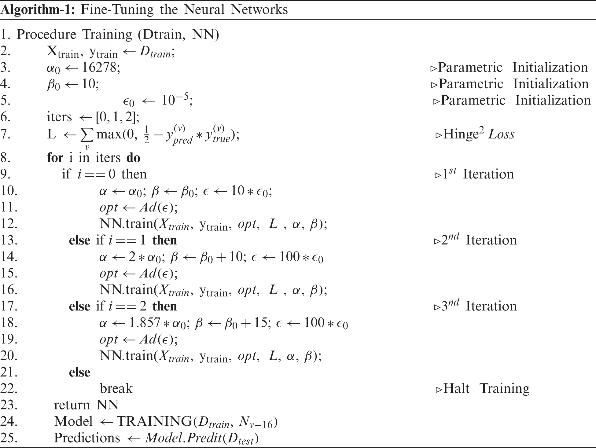
The training of an end-to-end CNN requires proper initializations, which can be computationally expensive. On the other hand, the transfer of weights from the pre-trained models for a similar problem statement can be useful to reduce the computational cost. However, they may not extract the invariances if the class samples in the problem statement are not trained at least once. For example, a pre-trained network on Imagenet may not be able to extract the invariances in CXRs if these samples are never seen or trained. This means that the model may end up capturing unwanted features on the CXR, leading to an inaccurate classification. In order to overcome this problem, the model is fine-tuned to obtain the appropriate features. Fine-tuning of the model is extremely important in medical imaging when the sample size is small, leading to class imbalance [31]. Hence, the existing models, starting from VGG-Nets to Dense-Nets, were all finetuned to extract invariant features and discriminate the COVID-19 class from the remaining. The fine-tuning for individual models were performed as per Algorithm-1. The major parameters considered for finetuning in our methodology were learning schedules and batch sizes. The algorithms were finetuned by constricting the noise caused during the training process to reduce the risk of misleading the model if not trained with appropriate initializations.
The Dtrain and Dtest samples were inserted into each model to capture latent feature vectors. A feedforward neural network was built to classify the extracted feature vectors, and all models were fine-tuned using Algorithm 1. The final extracted feature vector consisted of different three-dimensional shapes according to the model. These latent representations were then classified by attaching a dense layer consisting of 256 neurons followed by dropout [32] and batch normalization [33] of the layers for regularization. The final layer consisted of a softmax activation layer with “c” neurons, whereby “c” represents the number of classes. The dropout percentage was set to 30%. A generalization assessment was performed for all individual models. ReLU [34] was used for the non-linearity construction of the model architecture for all the layers except the final layer, whereby feed was forwarded by softmax. Glorot-normal was used for the initializations of most of the layers [35]. The initializations with appropriate activations resulted in the extraction of the following intricate, deep feature layers.
All models were carefully finetuned, and their performance was evaluated using various performance metrics. The generalizations provided by the finetuned models are summarized in Tab. 1. All the models performed well and had a similar overall performance Tab. 2. The classwise performance of the model is also summarized in Tab. 2. The classes are coded as C-0, C-1, and C-2, indicating COVID-19, normal, and pneumonia, respectively.


In the design of medical diagnostic prediction models, receiver operating characteristics (ROC) analysis is essential for analyzing the model performance. The area under the curve (AUC) of the ROC of a classifier determines the diagnostic stability of the model. This AUC-ROC curve is insensitive to the alterations in the individual class distributions [36]. A ROC curve for each model was therefore plotted, as shown in Fig. 4. The feature extraction ability of models varied widely, as not all models were capable of recognizing features pertaining to COVID-19 lesions.

Figure 4: AUC ROC curves obtained from the fine-tuned neural networks
A prediction model for medical imaging needs to have a high sensitivity and specificity. A clinically useful COVID-19 model based on CXR needs to be able to differentiate between COVID-19 from other infections. However, the distinction of CXR lesions caused by COVID-19 as opposed to other infections can be quite challenging. CAMs were therefore applied to all CXR input images [37]. CAMs apply global average pooling for bottleneck activations in CNNs and provide a visual understanding of discriminative image regions and/or the region of interest. CAMs provide a visual illustration through the use of heat maps of the features extracted by the models to make predictions. Therefore CAMs provide a clear understanding of whether the acquired features are distinctive of a COVID-19 lesion, as illustrated in Fig. 5.

Figure 5: Class activation maps (CAMs) obtained from the finetuned neural networks (a) Original CXR, (b) CAMs of VGG-16, (c) CAMs of VGG-19, (d) CAMs of InceptionV3 (e) CAMs of ResNet50, (f) CAMs of ResNet101, (g) CAMs of ResNet152, (h) CAMs of Xception, (i) CAMs of InceptionResNets, (j) CAMs of MobileNet, (k) CAMs of NasNetMobile, (l) CAMs of DenseNet121 (m) CAMs of DenseNet169, (n) CAMs of DenseNet201
The CAMs analysis shows that some of the models extract the peripheral and bilateral ground-glass opacities while some of the other models also extracted the rounded morphology typical of COVID-19 lesions [38]. Since both features were deemed essential for an accurate diagnosis, the models that provided the highest generalization and extracted different features according to the CAMs analysis were used to develop the neural model averaging or neural stacked ensembles models.
Model averaging is the process of averaging the outcomes of a group of networks trained on a similar task or the same model trained on different parameters. The model averaging improves the generalization of the models by aggregating their predictions. The generalization for the model was obtained by minimizing the loss during stochastic optimization using equation Eq. (1), whereby x and y are features and ground truth class labels of particular data distribution. If fn is an nth neural architecture that predicts the class label for a given feature set (where,
where
Similarly, weights can be assigned to individual models based on their prediction performance. These weights are then applied to the appropriate models to obtain aggregated generalization. This is known as weighted model averaging. In the case of model averaging, the models are equally treated by assigning the individual performance of the model to each network. This means that the weighted model averaging provides importance to the required models and discards the poorly performing models.
where
The generalization provided by the committee of the neural models improves when compared to that of model averaging and weighted model averaging. Hence, the models were stacked to improve the generalization ability of the model.
The stacked ensemble integrates or groups different models to provide aggregated generalization by mapping the output predictions onto a logit function. Instead of averaging the weights to the grouped models, logistic regression or multi-class logit was applied to map the predictions. Therefore, the predictions were gathered, and a logistic regression was applied to them or built at the end-to-end neural model that applies softmax non-linearity as final activation [39,40]. The generalization improvements provided by the stacked ensemble (using neural networks) were mathematically described as follows.
Our network was first considered to be a function that predicts a certain input x, where our true function is
where
So, the average individual error settled from the networks can be estimated as follows:
The ensemble learning of the grouping variant networks is presented in the following equations:
Estimated error resided by stacking these ensembles:
Suppose,
If individual networks did not correlate themselves, the stacking ensemble was reduced by n factors using the original generalization attained from the individual networks. However, for most scenarios, a correlation in generalization occurs, leading to an increase in the generalization error to a certain extent.
To understand this scenario,
This constant ‘
With this knowledge, it is clear that the stacked ensembles can outperform single networks in terms of generalization. As a result, six different neural network committees were formed by multiplying the number of neural networks described in Tab. 3, which ranged from 2 to 13 networks (all). These ensemble networks were evaluated using the standard classification metrics. A small neural architecture was attached to the committee of networks to adjoin the connected layer fully. This fully CNN consists of 16 neurons with a dropout of 30% for regularization. The final activations were pushed with softmax non-linearity, which consisted of three neurons describing the class predictions pertaining to each individual class. The results obtained by the proposed stacked ensembles are described in the next section in detail.

As mentioned, the generalization error obtained by a committee of neural networks is always less to that of a single neural network. Six variant committees of networks were selected and combined as described in Tab. 3. The classwise classification metrics utilized to understand the behavior of a specific COVID-19 class are illustrated in Tab. 4.

A comparative study was then performed to compare the performance of the proposed network with other existing models described in the literature Tab. 5.
Our designed generic training algorithm facilitates the training process by acquiring faster convergence and with low computations (Iterations). During the training process, the batch size and learning rate are increased cautiously for each iteration to obtain a balanced criterion, as explained by Smith et al. [41]. As noise during training can be reduced by properly choosing the batching parameters fed into the network, the learning rate and momentum of the optimizer were assigned a faster search.

The noise due to training is theoretically represented as follows in Eq. (18).
Here we assumed a constant momentum. A training algorithm was developed to conceptualize the noise constraint. Although a decaying learning rate can decrease the noise, it gradually increases the computational time for training. On the other hand, lowering the batch size can also reduce noise but comes at the cost of lowering the generalizing capacity of the model. These problems were overcome by developing an algorithm that increased the batch size during the specified iteration and cautiously increasing the learning rate as follows. The algorithm was first iterated for 16278 steps (iteration 1), whereby the learning rate was set to 10−4 by sending 15 samples as a batch at a time. In the next iteration (iteration 2), the batch size was increased by 50%, and the learning rate was increased tenfold. In order to maintain a consistent trade-off between generalization and faster convergence, the batch size was increased by a factor of 150% (to that of initial), and the learning rate was tuned as per the preceding iteration. During the experimentation, it was found that the proposed training procedure led to a faster convergence by training using only a few steps (approximately 20 epochs).
Appropriate training with fine-tuning of the ensemble was therefore critical to obtain these insightful outcomes. The final Ensemble-6 model had the highest performance when compared with the other method, with an accuracy score of 99.175%. Ensemble-1 and Ensemble-2 attained an accuracy of 98.487% and 98.762%, respectively. When taking into consideration only the COVID-19 class, the precision rate was at least 97.674%, but the recall rate was lower. The highest and lowest recall rates were 89.795% and 69.387% and were obtained by Ensemble-6 and Ensemble-4, respectively. However, due to the small sample of the COVID-19 class in our study, it was difficult to extract additional invariant features to improve the performance of the model further.
In this study, we observed that the stacked ensemble was slightly inefficient when a poor-performing model was included. The DenseNet-201 model evaluations were not always finetuned correctly, and the network depth was not always appropriate, leading to a high generalization error. The COVID-19 results were not always included in the single model based on the features derived from the individual models. The ensemble method offers more generalization, but the combination of multiple models increased the computational cost, which is unnecessary for small-scale computational systems (such as Ensemble-6). As a result, in real-world scenarios, small, quick, and efficient models such as Ensemble-1 and Ensemble-2 are advantageous. The progression of the virus can be visualized better on Chest CT axial images. However, there is a chance of missing disease progression on CXR [38], which could be dangerous. Therefore future studies should focus on the development of models that can predict disease progression on CXR.
In this study, various COVID-19 classification models were evaluated and compared using different classification metrics. Furthermore, a learning framework for finetuning these models was proposed, and their bottleneck activations were visualized using CAMs. The AUC-ROC curves were closely examined, and the output of each class was illustrated visually. These fine-tuned models were then stacked to outperform previous models and include a broad range of generalizations. The ensemble models achieve an accuracy score of 97.66 percent in the worst-case scenario. Even after finetuning for class imbalance, the models were found to have a high generalization ability. The least error rate obtained by the outperforming model, built by stacking all the finetuned models, was 0.83%. The stacked ensembles method improved the performance of the model and could therefore be used to improve the prediction accuracy of the diagnostic models in medical imaging.
Acknowledgement: The authors extend their appreciation to King Saud University for funding this work through Researchers Supporting Project number RSP-2021/305, King Saud University, Riyadh, Saudi Arabia.
Funding Statement: The research is funded by the Researchers Supporting Project at King Saud University, (Project# RSP-2021/305).
Conflicts of Interest: The authors declare that they have no conflicts of interest to report regarding the present study.
1. C. Sohrabi, Z. Alsafi, N. O'Neill, M. Khan, A. Kerwan et al., “World health organization declares global emergency: A review of the 2019 novel coronavirus (COVID-19),” International Journal of Surgery, vol. 76, pp. 71–76, 2020. [Google Scholar]
2. F. Pan, T. Ye, P. Sun, S. Gui, B. Liang et al., “Time course of lung changes at chest CT during recovery from coronavirus disease 2019 (COVID-19),” Radiology, vol. 295, no. 3, pp. 715–721, 2020. [Google Scholar]
3. F. Zhou, T. Yu, R. Du, G. Fan, Y. Liu et al., “Clinical course and risk factors for mortality of adult inpatients with COVID-19 in wuhan, China: A retrospective cohort study,” The Lancet, vol. 395, no. 10229, pp. 1054–1062, 2020. [Google Scholar]
4. Z. Li, Y. Yi, X. Luo, N. Xiong, Y. Liu et al., “Development and clinical application of a rapid IgM-IgG combined antibody test for SARS-CoV-2 infection diagnosis,” Journal of Medical Virology, vol. 92, no. 9, pp. 1518–1524, 2020. [Google Scholar]
5. C. Rothe, M. Schunk, P. Sothmann, G. Bretzel, G. Froesch et al., “Transmission of 2019-nCoV infection from an asymptomatic contact in Germany,” New England Journal of Medicine, vol. 382, no. 10, pp. 970–971, 2020. [Google Scholar]
6. Y. Bai, L. Yao, T. Wei, F. Tian, D. Y. Jin et al., “Presumed asymptomatic carrier transmission of COVID-19,” Jama, vol. 323, no. 14, pp. 1406–1407, 2020. [Google Scholar]
7. Y. LeCun, Y. Bengio and G. Hinton, “Deep learning,” Nature, vol. 521, no. 7553, pp. 436–444, 2015. [Google Scholar]
8. D. P. Fan, T. Zhou, G. P. Ji, Z. Yi, G. Chen et al., “Inf-net: Automatic covid-19 lung infection segmentation from ct images,” IEEE Transactions on Medical Imaging, vol. 39, no. 8, pp. 2626–2637, 2020. [Google Scholar]
9. Y. Oh, S. Park and J. C. Ye, “Deep learning covid-19 features on CXR using limited training data sets,” IEEE Transactions on Medical Imaging, vol. 39, no. 8, pp. 2688–2700, 2020. [Google Scholar]
10. M. Rahimzadeh and A. Attar, “A modified deep convolutional neural network for detecting COVID-19 and pneumonia from chest X-ray images based on the concatenation of xception and resnet50v2,” Informatics in Medicine Unlocked, vol. 19, pp. 100360, 2020. [Google Scholar]
11. T. Ozturk, M. Talo, E. A.Yildirim, U. B. Baloglu and Y. Ozal et al., “Automated detection of COVID-19 cases using deep neural networks with X-ray images,” Computers in Biology and Medicine, vol. 121, pp. 103792, 2020. [Google Scholar]
12. I. D. Apostolopoulos and T. A. Mpesiana, “Covid-19: Automatic detection from x-ray images utilizing transfer learning with convolutional neural networks,” Physical and Engineering Sciences in Medicine, vol. 43, no. 2, pp. 635–640, 2020. [Google Scholar]
13. L. Li, L. Qin, Z. Xu, Y. Yin, X. Wang et al., “Artificial intelligence distinguishes COVID-19 from community-acquired pneumonia on chest CT,” Radiology, vol. 296, no. 2, pp. E65–E71, 2020. [Google Scholar]
14. A. I. Khan, J. L. Shah and M. M. Bhat, “Coronet: A deep neural network for detection and diagnosis of COVID-19 from chest x-ray images,” Computer Methods and Programs in Biomedicine, vol. 196, pp. 1–9, 2020. [Google Scholar]
15. G. Wang, X. Liu, C. Li, Z. Xu, J. Ruan et al., “A noise-robust framework for automatic segmentation of COVID-19 pneumonia lesions from CT images,” IEEE Transactions on Medical Imaging, vol. 39, no. 8, pp. 2653–2663, 2020. [Google Scholar]
16. Lalith-Bharadwaj-B/COVID-19-Datasets. [Online]. Available: https://github.com/LalithBharadwaj/COVID-19-Datasets, 2021. [Google Scholar]
17. Y. Bengio, A. Courville and P. Vincent, “Representation learning: A review and new perspectives,” IEEE Transactions on Pattern Analysis and Machine Intelligence, vol. 35, no. 8, pp. 1798–1828, 2013. [Google Scholar]
18. A.Krizhevsky, I. Sutskever and G. E., Hinton, “Imagenet classification with deep convolutional neural networks,”Advances in Neural Information Processing Systems, vol. 25, pp. 1097–1105, 2012. [Google Scholar]
19. I. J. Goodfellow, J. Pouget-Abadie, M. Mirza, B. Xu, D. Warde-Farley et al., “Generative adversarial networks,” ArXiv Preprint ArXiv: 406–2661, 2014. [Google Scholar]
20. S. J. Pan and Q. Yang, “A survey on transfer learning,” IEEE Transactions on Knowledge and Data Engineering, vol. 22, no. 10, pp. 1345–1359, 2009. [Google Scholar]
21. W. Dai, Q. Yang, G. R. Xue and Y. Yu, “Boosting for transfer learning,”, in Proc. of the 24th Int. Conf. on Machine Learning, ICML 2007, Oregon State University in Corvallis, Oregon, USA, ACM, pp. 193–200, 2007. [Google Scholar]
22. C. Szegedy, W. Liu, Y. Jia, P.Sermanet, R. Scott et al., “Going deeper with convolutions”, in Proc. of the IEEE Conf. on Computer Vision and Pattern Recognition, pp. 1–9, 2015. [Google Scholar]
23. K. Simonyan and A. Zisserman, “Very deep convolutional networks for large-scale image recognition,” arXiv preprint arXiv: 1409-1556, 2014. [Google Scholar]
24. K. He, X. Zhang, S. Ren and J. Sun, “Deep residual learning for image recognition,” in Proc. of the IEEE Conference on Computer Vision and Pattern Recognition, pp. 770–778, 2016. [Google Scholar]
25. C. Szegedy, S. Ioffe, V. Vanhoucke and A. Alemi, “Inception-v4, inception-resnet and the impact of residual connections on learning,” in Proc. of the AAAI Conf. on Artificial Intelligence, San Francisco, California, USA, vol. 31, no. 1, 2017. [Google Scholar]
26. K. He, X. Zhang, S. Ren and J. Sun, “Identity mappings in deep residual networks,” in European Conference on Computer Vision, pp. 630–645, Springer, Cham, 2016. [Google Scholar]
27. F. Chollet, “Xception: deep learning with depthwise separable convolutions,” in Proc. of the IEEE Conference on Computer Vision and Pattern Recognition, Hawai‘i Convention Center, Honolulu, Hawaii, United States, pp. 1251–1258, 2017. [Google Scholar]
28. G. Huang, Z. Liu, L. V. Der Maaten and Q. W. Kilian, “Densely connected convolutional networks,” in Proc. of the IEEE Conference on Computer Vision and Pattern Recognition, Hawai‘i Convention Center, Honolulu, Hawaii, United States, pp. 4700–4708, 2017. [Google Scholar]
29. M. Sandler, A. Howard, M. Zhu, Z. Andrey and L. C., Chen, “Mobilenetv2: inverted residuals and linear bottlenecks,” in Proc. of the IEEE Conference on Computer Vision and Pattern Recognition, Salt Lake City, UT, USA, pp. 4510–4520, 2018. [Google Scholar]
30. B. Zoph, V. Vasudevan, J. Shlens and Q. V. Le, “Learning transferable architectures for scalable image recognition,” in Proc. of the IEEE Conference on Computer Vision and Pattern Recognition, Salt Lake City, UT, USA, pp. 8697–8710, 2018. [Google Scholar]
31. N. Tajbakhsh, J. Y. Shin, S. R. Gurudu, R. T. Hurst, C. B. Kendall et al., “Convolutional neural networks for medical image analysis: Full training or fine-tuning?,” IEEE Transactions on Medical Imaging, vol. 35, no. 5, pp. 1299–1312, 2016. [Google Scholar]
32. N. Srivastava, G. Hinton, A. Krizhevsky, I. Sutskeve and R. Salakhutdinov, “Dropout: A simple way to prevent neural networks from overfitting,” The Journal of Machine Learning Research, vol. 15, no. 1, pp. 1929–1958, 2014. [Google Scholar]
33. S. Ioffe and C. Szegedy, “Batch normalization: Accelerating deep network training by reducing internal covariate shift,” in Int. Conference on Machine Learning, Lille, France, pp. 448–456, PMLR, 2015. [Google Scholar]
34. V. Nair and G. E. Hinton, “Rectified linear units improve restricted boltzmann machines”, in Proc. of the 27th Int. Conference on Machine Learning, Haifa, Israel, 2010. [Google Scholar]
35. X. Glorot and Y. Bengio, “Understanding the difficulty of training deep feedforward neural networks,” in Proc. of the Thirteenth Int. Conf. on Artificial Intelligence and Statistics, JMLR Workshop and Conference Proceedings,, Sardinia, Italy, pp. 249–256, 2010. [Google Scholar]
36. B. Zhou, A. Khosla, A. L. Lapedriza, A. Oliva and A. Torralba, “Learning deep features for discriminative localization,” in Proc. of the IEEE Conference on Computer Vision and Pattern Recognition, Caesars Palace, Las Vegas, Nevada, United States, pp. 2921–2929, 2016. [Google Scholar]
37. T. Fawcett, “An introduction to ROC analysis.” Pattern Recognition Letters, vol. 27, no. 8, pp. 861–874, 2006. [Google Scholar]
38. H. Y. F. Wong, H. Y. S. Lam, A. H. T. Fong, S. T. Leung, T. W. Y. Chin et al., “Frequency and distribution of chest radiographic findings in patients positive for COVID-19,” Radiology, vol. 296, no. 2, pp. E72–E78, 2020. [Google Scholar]
39. L. K. Hansen and P. Salamon, “Neural network ensembles,” IEEE Transactions on Pattern Analysis and Machine Intelligence, vol. 12, no. 10, pp. 993–1001, 1990. [Google Scholar]
40. A. Krogh and J. Vedelsby, “Neural network ensembles, cross-validation, and active learning.” Advances in Neural Information Processing Systems, vol. 7, no. 7, pp. 231–238, 1995. [Google Scholar]
41. S. L. Smith, P. J. Kindermans, C. Ying and Q. V. Le, “Don't decay the learning rate, increase the batch size,” arXiv preprint arXiv:1711.00489, 2017. [Google Scholar]
 | This work is licensed under a Creative Commons Attribution 4.0 International License, which permits unrestricted use, distribution, and reproduction in any medium, provided the original work is properly cited. |