Computers, Materials & Continua DOI:10.32604/cmc.2022.020583
Article

Swarm-Based Extreme Learning Machine Models for Global Optimization

Mustafa Abdul Salam1,*, Ahmad Taher Azar2 and Rana Hussien2

1Artificial Intelligence Department, Faculty of Computers and Artificial Intelligence, Benha University, Benha, 13518, Egypt
2Scientific Computing Department, Faculty of Computers and Artificial Intelligence, Benha University, Benha, 13518, Egypt
*Corresponding Author: Mustafa Abdul Salam. Email: mustafa.abdo@fci.bu.edu.eg
Received: 30 May 2021; Accepted: 29 July 2021

Abstract: Extreme Learning Machine (ELM) is popular in batch learning, sequential learning, and progressive learning, due to its speed, easy integration, and generalization ability. While, Traditional ELM cannot train massive data rapidly and efficiently due to its memory residence, high time and space complexity. In ELM, the hidden layer typically necessitates a huge number of nodes. Furthermore, there is no certainty that the arrangement of weights and biases within the hidden layer is optimal. To solve this problem, the traditional ELM has been hybridized with swarm intelligence optimization techniques. This paper displays five proposed hybrid Algorithms “Salp Swarm Algorithm (SSA-ELM), Grasshopper Algorithm (GOA-ELM), Grey Wolf Algorithm (GWO-ELM), Whale optimization Algorithm (WOA-ELM) and Moth Flame Optimization (MFO-ELM)”. These five optimizers are hybridized with standard ELM methodology for resolving the tumor type classification using gene expression data. The proposed models applied to the predication of electricity loading data, that describes the energy use of a single residence over a four-year period. In the hidden layer, Swarm algorithms are used to pick a smaller number of nodes to speed up the execution of ELM. The best weights and preferences were calculated by these algorithms for the hidden layer. Experimental results demonstrated that the proposed MFO-ELM achieved 98.13% accuracy and this is the highest model in accuracy in tumor type classification gene expression data. While in predication, the proposed GOA-ELM achieved 0.397which is least RMSE compared to the other models.

Keywords: Extreme learning machine; salp swarm optimization algorithm; grasshopper optimization algorithm; grey wolf optimization algorithm; moth flame optimization algorithm; bio-inspired optimization; classification model; and whale optimization algorithm

1  Introduction

In recent years, Extreme Learning machine (ELM) has attracted a significant attention in a range of fields as an accurate and powerful machine learning technique. ELM is a less-square learning algorithm for a ‘general’ single-hidden layer feedforward network (SLFN) that can be used as an estimator or as a classifier in a regression problem. ELM has two major advantages: easier to understand and excellent results in generalization. ELM has also been used to carry out many studies in the fields of image applications filter design, market predictions, time series forecasting, energy efficiency shipping, electricity load prediction, target detection, aircraft reconnaissance, clustering, real-time error diagnostics, end-point prediction model, design of neural architectures, illness diagnosis, agility prevision, etc [1].

The Single Hidden Layer Neural Feed Forward (SLFN) is commonly considered as one of the most popular learning machine models in the classification and prediction areas. The Learning Algorithm is widely acknowledged to be at the core of the Neural Network [2]. Traditional gradient-based machine learning approaches, such as Levenberg-Marquardt (LM) and Scaled-Conjugate-Gradient (SCG), complain about over-fitting, minima local, and long-term waste memory [3]. ELM [4] has been presented to fix complex issues mentioned in gradient-based machine learning algorithms. ELM is used as an SLFN learning solution. Although many real-life problems have been arisen, ELM has enormous precision and anticipation speed [5]. Instead of turning all inner parameters as in gradient-based algorithms, ELM efficiently determines the weight of inputs and the bias of the hidden layer. ELM also assists in offering an unbiased overview of the output weight. Gradient-based learning algorithms need less hidden neurons than ELM due to the erratic choice of input weights and hidden layer bias [6,7].

1.1 Motivations and Contributions

Machine learning (ML) has proven to be useful in tackling tough issues in classification and prediction. ELM, one of the machine learning algorithms that requires significantly shorter training time than popular Back Propagation (BP) and support vector machine/support vector regression (SVM/SVR) [8]. In many situations, the prediction accuracy of ELM is somewhat greater than that of BP and close to that of SVM/SVR. In comparison to BP and SVR, ELM is easier to construct since there is few parameters to tune. ELM requires more hidden nodes than BP but many fewer than SVM/SVR, implying that ELM and BP respond to unknown input considerably faster than SVM/SVR. ELM has an incredibly rapid learning rate. In contrast to standard gradient-based learning methods, which only operate with differentiable activation functions. Unlike standard gradient-based learning algorithms, which have numerous difficulties such as local minima, inappropriate learning rate, and overfitting, etc., ELM tends to achieve simple answers without such minor issues. Many learning algorithms, such as neural networks and support vector machines, appear considerably easier than the ELM learning method. The ELM's obstacles overcame, by using bio-inspired algorithms to refine it.

Five bio-inspired algorithms are proposed to optimize ELM model. These algorithms are namely, Salp Swarm Optimizer (SSA) [9], Grasshopper Optimizer (GOA) [10], Grey Wolf Optimizer (GWO) [11], Moth Flame Optimizer (MFO) [12] and Whale Optimizer (WOA) [13]. These algorithms have been used to select input weights and biases in order to define ELM weights of the output. Proposed models performed a significant generalization of the simplified structure. They have been used to identify the quality of motions of patients with distinctive tumor forms and their advanced identification. Also, they have been used to predict the electricity consumption of Clients.

1.2 Paper Organization

The paper is structured as follows: Section 2 devoted for related work. Section 3 presents preliminaries that describe (SVM, ELM and the swarm intelligence algorithms); Section 5 reflects on the potential approach and the implementation of hybrid models; Section 6 discusses the experimental results, while Section 7 points out the core conclusions of the proposed model and highlights the future work.

2  Related Work

Wang et al. [8] investigated the efficacy of the ELM and suggested a revised effectiveness of extreme learning algorithm. The suggested algorithm requires an optimal set of input weights and assumptions, ideally maintaining the full column rank of H matrix. Isham et al. [14] used a whale optimization algorithm (WOA) technique to determine the optimal value of the input weight and the hidden layer distortions. Huang et al. [15] proposed a new learning algorithm called the ELM for single-hidden layers feedforward neural networks (SLFNs), which randomly chooses hidden nodes and analytically measures SLFN output weights. This algorithm generalized at an extremely high pace in theory while studying. Using ELM ideas. HuaLing et al. [16] increased the performance of ELM convergence by integrating ELM and PSO algorithm. Alhamdoosh et al. [17] presented an evolutionary approach that was defined for the assembly of ELM to reach an optimal solution while preserving the size of the ensemble under control. Wu et al. [18] used GA algorithm to optimize ELM model. Sundararajanc et al. [19] used a truly modern genetic algorithm called ‘RCGA ELM’ to pick out the strongest neurons in the hidden layer. Zhao et al. [20] suggested a genetic ELM focused on the economic distribution of the power grid. Abdul Salam et al. [21] refined the ELM model and increased efficiency in stock market forecasts compared to the classic ELM model, as well as they suggested a new Flower Pollination Algorithm (FPA). Salam et al. [22] stated that in this model, the dragonfly optimizer applied a hybrid dragonfly algorithm with an extreme predictive learning scheme, which improved the ELM model's predictive performance. According to Aljarah et al. [23], the proposed WOA-based training algorithm outperforms existing algorithms in most datasets; not only in terms of accuracy, but also in terms of convergence. Mohapatra et al. [24] discovered that ELM-based classifiers work better when projecting higher dimensional space elements. Liu et al. [25] proposed a multi-extension of the kernel ELM to manage heterogeneous databases through kernel tuning and convergence. According to Huang et al. [26], the separating hyperplane begins to travel through the root of the ELM's space function, resulting in less space. SVM has less optimization limitations and improved generalization performance. It was also noted that there is a generalization of the ELM's output that is less sensitive to learning parameters such as the number of hidden nodes. Zong et al. [27] demonstrated that the weighted ELM is capable of balanced data generalization. Sowmya et al. [28] designed sensor system uses the spectroscopic method using machine learning to improve the accuracy of detection.

3  Preliminaries

3.1 Extreme Learning Machine (ELM)

The Extreme learning machine for training SLFN was proposed by Huang et al. [15]. ELM's central idea is the hidden weights of the layer. In addition, the biases are generated randomly, with the less-squares procedure used to determine the output weights. The outputs of the objectives and the hidden layer [29] are also established. Fig. 1 shows a high-level outline of the training algorithm and the ELM layout. Where: N refers to a set of unique samples (Xi,ti), where Xi = [xi1,xi2…xin]T ∈ Rn and ti= [ti1,ti2…tim]T∈ Rm, L represents the hidden layer nodes, g(x) represents the activation function,

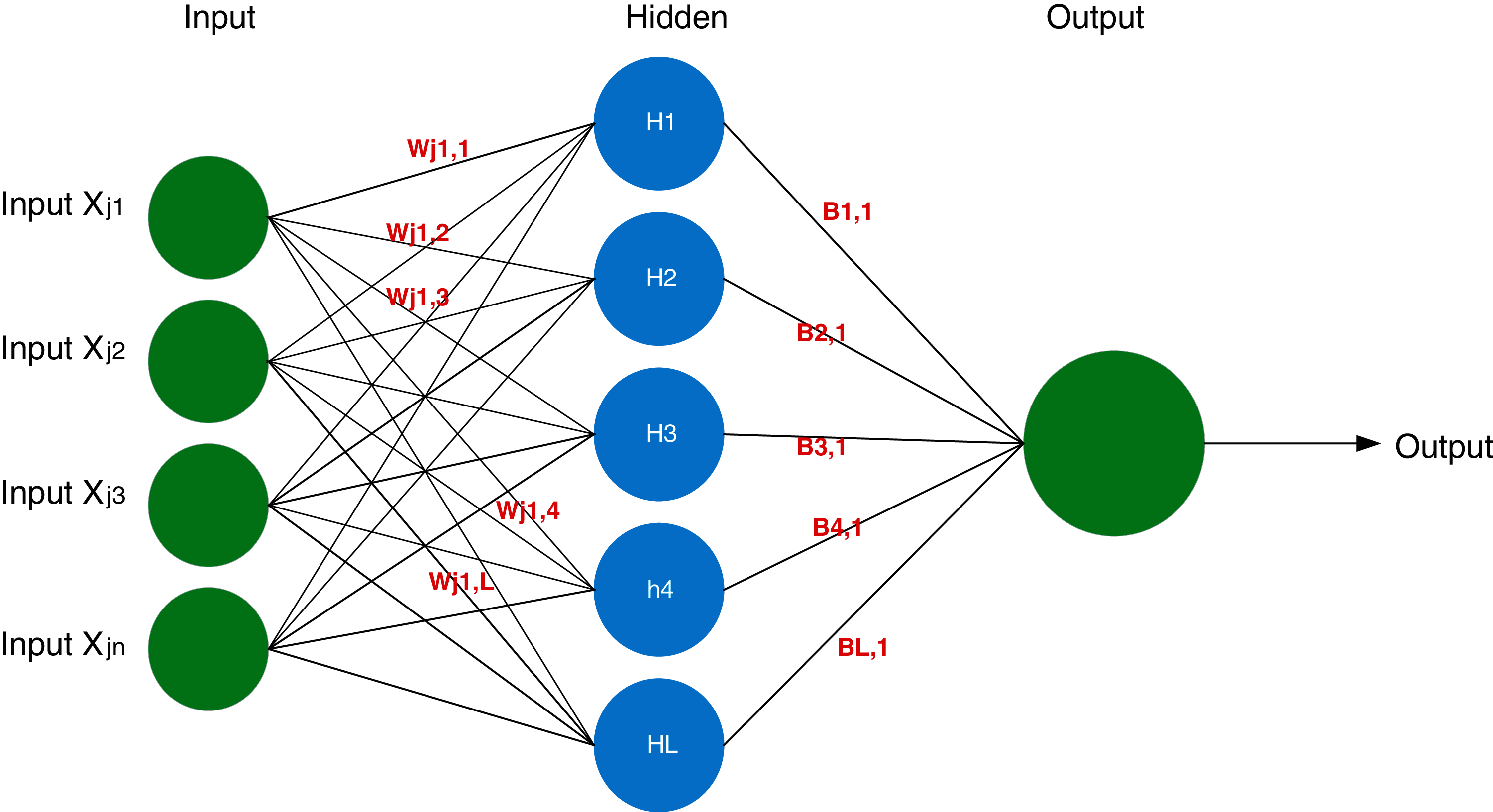
Figure 1: Diagram of ELM (Huang et al. 2011)

There is also a mathematical model represented as shown in Eq. (1):

∑i=1L⁡βigi(Xj)=∑i=1Lβigi(Wi.Xj+bi)(1)

where: Wi = [Wi1,Wi2…Win]T represents the vector of weight connecting the hidden node and the ith nodes, βi = [βi1,βi2…βim]T represents the vector weight which connects the hidden nodes to the output nodes, bi It represents the threshold of the hidden nodes, Wi. Xj represents the inner product of Wi and Xj.S election of the output nodes is linearly done, however.

The SLFN and L hidden nodes norm in the g(x) activation function is error-free. In other words, mean: ∑j=1L⁡ || oj−tj|| = 0, i.e., and there exist βi,Wi  and bi in such a way that declared in Eq. (2)

∑i=1Lβigi(WiXj+bj)=tj,j=1,…N,(2)

It can then be presented as represented in Eq. (3)

Hβ=T(3)

where we can represent H Matrix as represented below in Eq. (4)

H(W1…WL,b1…bL,X1…XN)=[g(W.1..X1+b1)⋯g(W.L..X1+bL)⋮⋮⋮g(W.1..XN+b1)⋯g(W.1..XN+bL)](4)

We can display β in Eq. (5) and T in Eq. (6)

β=[β1TβLT]L∗m(5)

T=[t1TtLNT]N∗m(6)

And Eq. (3) becomes a linear system. Furthermore, by finding a least square solution, the performance weights β can be calculated analytically: β = Where the generalized inverse for H Moore–Penrose.

This results in a mathematical transformation in the weighing of the items. This ensures that a change in network parameters for such basic learning parameters eliminates the long training time (such as iterations and learning rate).

A number of variables were described, Huang et al. (2006), The H matrix in which the hidden layers are represented and the ith column determines the hidden layer input nodes. The activation function g becomes infinitely differentiable if L ≤ N represents the optimal number of hidden nodes.

3.2 Swarm Intelligence Algorithms

3.2.1 Salp Swarm Algorithm (SSA)

Salp Swarm Algorithm (SSA) was proposed by Mirjalili et al. [9]. The main inspiration of SSA is the swarming behaviour of salps when navigating and foraging in oceans. The society is divided into two groups: leaders and followers to model the salp chains mathematically. The salp is the leader in the front chain, while the remaining salp followers are called.

The leader's position can be updated according to Eq. (7) as follows:

xj1={Fj+c1((ubj−lbj)c2+lbjFj−c1((ubj−lbj)c2+lbj(7)

where xj1 represents the position of the first salp (leader) in the jth dimension, Fj is the position of the food source in the jth dimension, ubj represents the upper bound of jth dimension, lbj represents the lower bound of jth dimension, c1, c2, and c3 are random numbers.

Eq. (8): Newton's law of motion was used to update the position of the followers:

xji=12at2+v0t(8)

where i ≥ 2, xji shows the position of ith follower salp in jth dimension, t is time, v0 is the initial speed, and a=vfinalv0 where v=x−x0t.

3.2.2 Grasshopper Optimization Algorithm (GOA)

Luo et al. [10] created the GOA, a new swarm intelligence algorithm. GOA is a system that is dependent on the population. GOA mimics the nature and social activity of grasshopper swarms.

Three forces determine each grasshopper's place in the swarm. Its social contact with the other grasshoppers Si, Gravitational effect on it Gi, and wind advection the letter Ai. The following Eq. (9) is the final shape of the three impacted powers on each grasshopper.

Xi=Si+Gi+Ai(9)

Eq. (10) explains the social interaction between each grasshopper and the other grasshopper.

Si=∑j=1N⁡s(dij)dij^,j≠1(10)

where dij is the distance between the grasshopperi and grasshopperj, s is a function represents the strength of two social force, attraction and repulsion between grasshoppers, it can be defined as represented in Eq. (11).

s(r)=fe−rl−e−r(11)

where f, l is the attraction strength and the attractive length dimension. The position of the grasshopper can be calculated as declared in Eq. (12):

Xi=∑j=1N⁡s(|xj−xi|)xj−xidij−geg^+uew^(12)

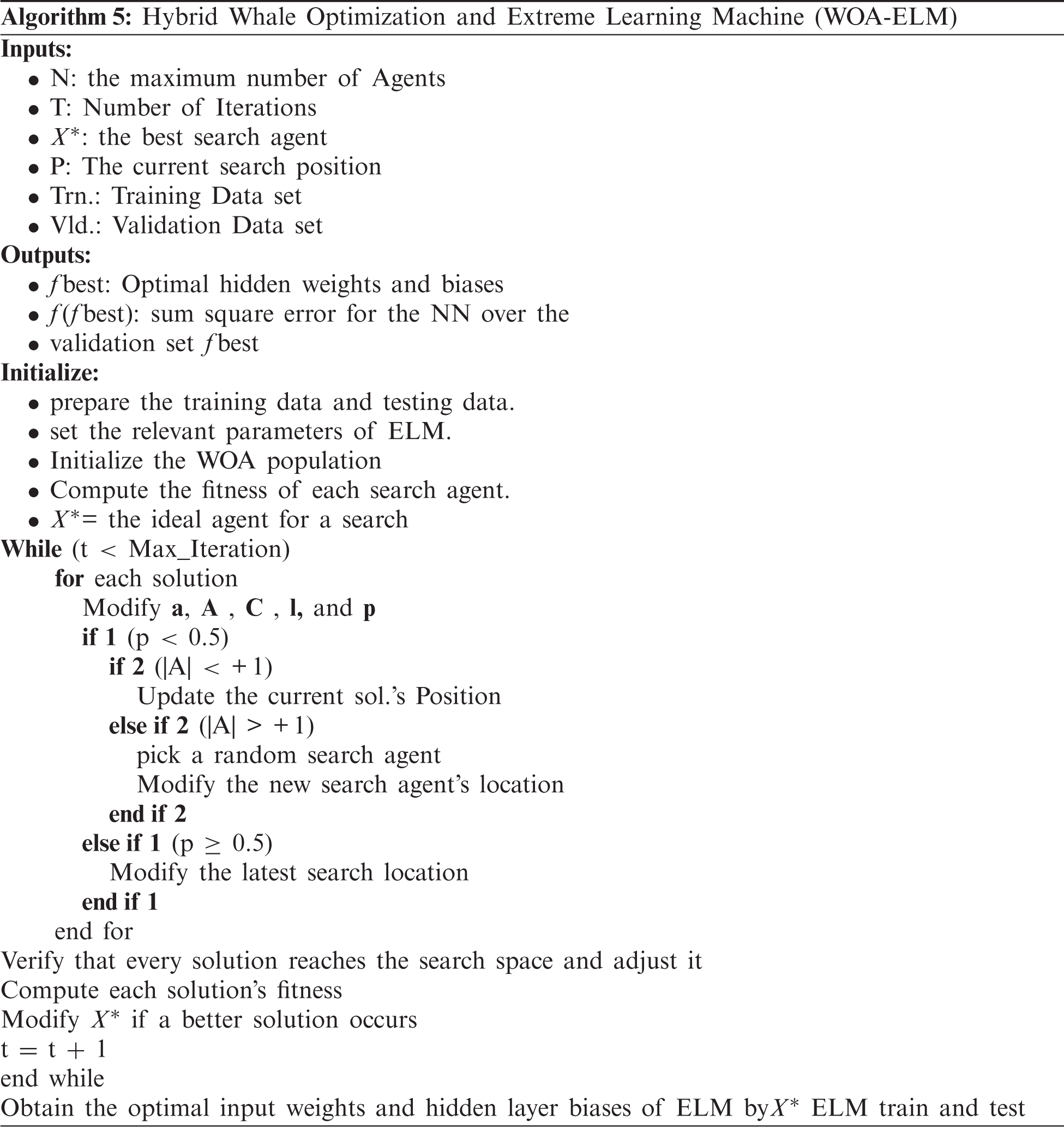
3.2.3 Whale Optimization Algorithm (WOA)

WOA could be a recent algorithm introduced in 2016 by Mirjalili et al. [13] on a population level. WOA is derived from the social activity of humpback whales.

The difference is determined between the whale at (X, Y) and the abuser at (X*, Y*). At this point, after the Helix-shaped forming of the Humpback whale, a winding condition is formed between the position of the whale and the victim to be taken as described below in Eqs. (13) and (14):

X→(t+1)=ebk.cos⁡(2πk).D∗→+X∗→(t),(13)

D∗→=|X∗→(t)−X→(t)|(14)

To retrieve the pattern of the logarithmic spiral, if B can be a constant value, and k can be an arbitrary number within the range [−1, 1]. This way, in the middle of optimization, WOA thinks about changing whaling. There is a 50 percent chance of choosing between the lease component and the contract portion, and the contract components are as represented in Eq. (15):

X→(t+1)={X∗→−A→.D→ebk.cos⁡(2πk).D∗→+X∗→(t),if p≥0.5,(15)

where p is a random number within the (0,1).

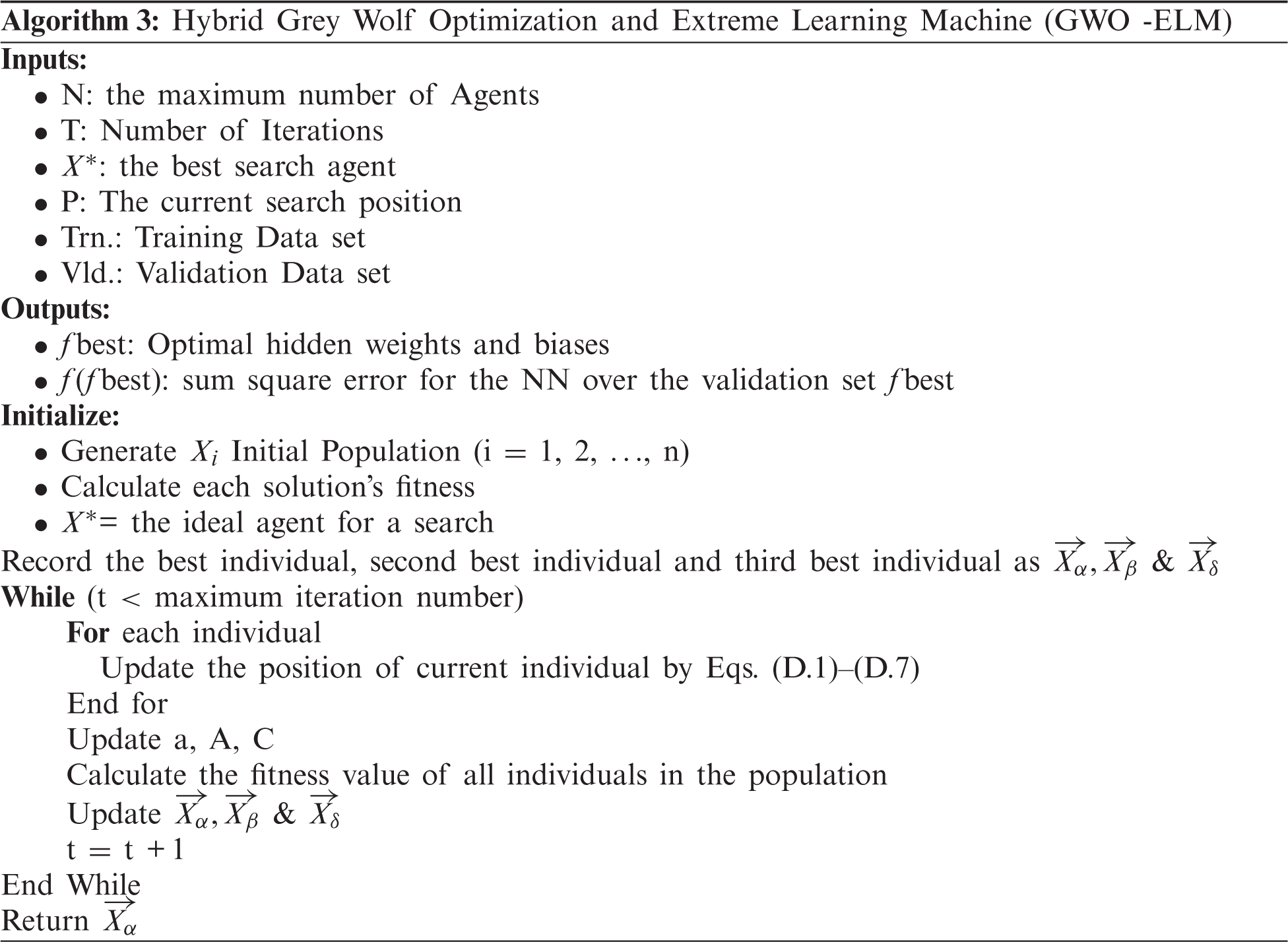
3.2.4 Grey Wolf Optimizer (GWO)

Seyedali Mirjalili and colleagues proposed the grey wolf optimizer (GWO) in 2014 as a novel swarm intelligent optimization algorithm that primarily imitates the hierarchy of wolf management and hunting in nature [30].

Mirjalili developed the optimization algorithm by modelling it after the looking and hunting actions of grey wolves. The optimum solution is defined as alpha (α), the second best as beta (β), and the third best as delta (β) for the mathematical model. Many of the remaining candidate solutions are omegas (ω). These three grey wolves will lead all the omegas when looking (optimizing) and shooting.

When a prey object is discovered, the iteration starts (t = 1). Following that, the alpha, beta, and delta wolves would lead the omegas in pursuing and ultimately encircling the prey. To define the encircling action, three coefficients are proposed as represent in Eqs. (16)–(18):

Dα→=|C1→.Xa→−X→(t)|,(16)

Dβ→=|C2→.Xβ→−X→(t)|,(17)

Dδ→=|C3→.Xδ→−X→(t)|,(18)

where t indicates the current iteration, X→ is the position vector of the grey wolf, and X1→ , X2→ & X3→ are the position vectors of the alpha, beta, and delta wolves. X→ would be computed as Eqs. (19)–(22):

X1→=Xa→−A1→.Dα→,(19)

X2→=Xβ→−A2→.Dβ→(20)

X3→=Xδ→−A3→.Dδ→(21)

X→(t)=X1→+X2→+X3→3(22)

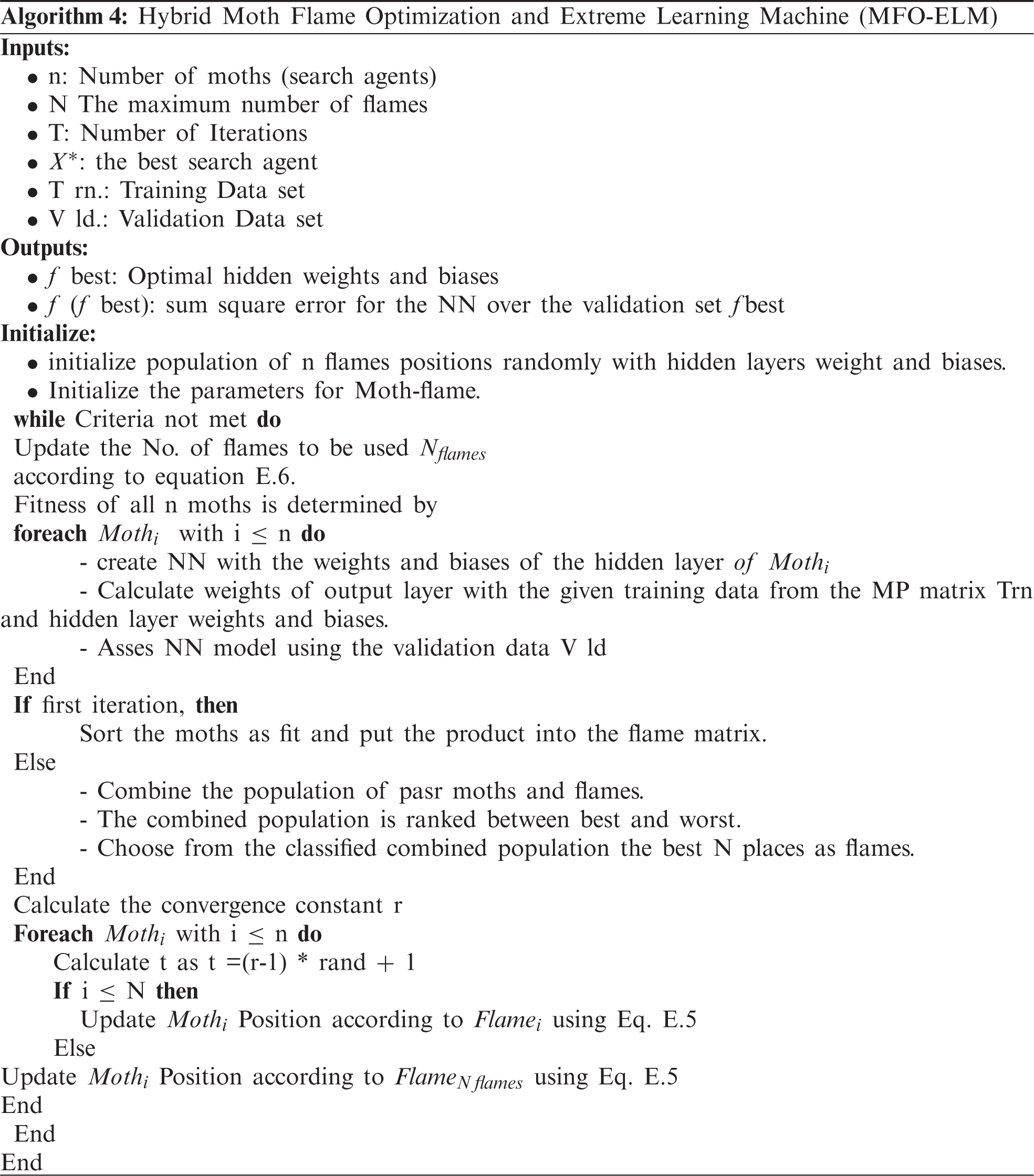
3.2.5 Moth–Flame Optimization Algorithm (MFO)

MFO is a new Metaheuristic population-based approach created by Mirjalili in 2015 [31] that mimics the transverse orientation for navigation technique used by moths at night. Moths travel at night dependent on the moonlight, keeping a set angle to navigate their way.

MFO starts by randomly creating moths in the solution space, then calculating each moth's fitness values (i.e., location) and labelling the best position with flame. The position of the moths is then updated with the spiral movement function to attain better flame marked locations, then the best individual location updates and the previous processes continue until the ends have been achieved. MFO converges the global optimum of optimization problems using three associated functions. The following are these functions as declared in Eq. (23):

MFO=(I,P,T)(23)

where I refers to the first random locations of the moths (I: Φ →{M, OM}), P refers to motion of the moths in the search space (P:M→M), and T refers to finish the search process (T: M→ true, false). Eq. (24) represents I function, which is used for implementing the random distribution.

M(i,j)=(ub(i)−lb(j)) ∗ rand()+lb(i)(24)

where lb and ub indicate the lower and upper bounds of variables, respectively.

The MFO algorithm's logarithmic spiral is as described in Eq. (25):

S(Mi,Fj)=Di.ebt.cos⁡(2πt)+Fj(25)

where Di refers to the space between the i-th moth and the j-th flame (i.e., Di=|Fi−Mi|), b indicates a fix to define the shape of the logarithmic spiral, and t indicates a random number between [−1, 1].

This section focuses on enhancing MFO algorithm exploitation (for example, updating the moths’ positions in n different locations in the search space will minimize the probability of exploiting the most promising solutions). Reducing the number of fires, as a consequence of the following Eq. (26), helps in the resolution of this problem:

flame no=round(N−l∗N−lT)(26)

where N denotes the maximum number of fires, l the present number of iterations, and T the cumulative number of iterations.

4  The Proposed Hybrid Models

As long as a suitable number of hidden nodes are selected within the program, ELMs offer the benefit of taking minimum training time while still preserving acceptable classification and predication. Since the optimum hidden layer weighting is not achievable within the hidden layer, the huge number of nodes slows down the execution of the ELM experiments. Therefore, in this hybrid model, fewer nodes within the hidden layer must be used to accelerate ELM execution while retaining an appropriate choice of hidden layer weights and predispositions. It is often used in the same manner when determining the weights and preferences of the output sheet. Swarm algorithms are the most efficient for collecting the hidden layer weights and expectations that optimize the overall execution of the ELM.

4.1 SSA-ELM Model

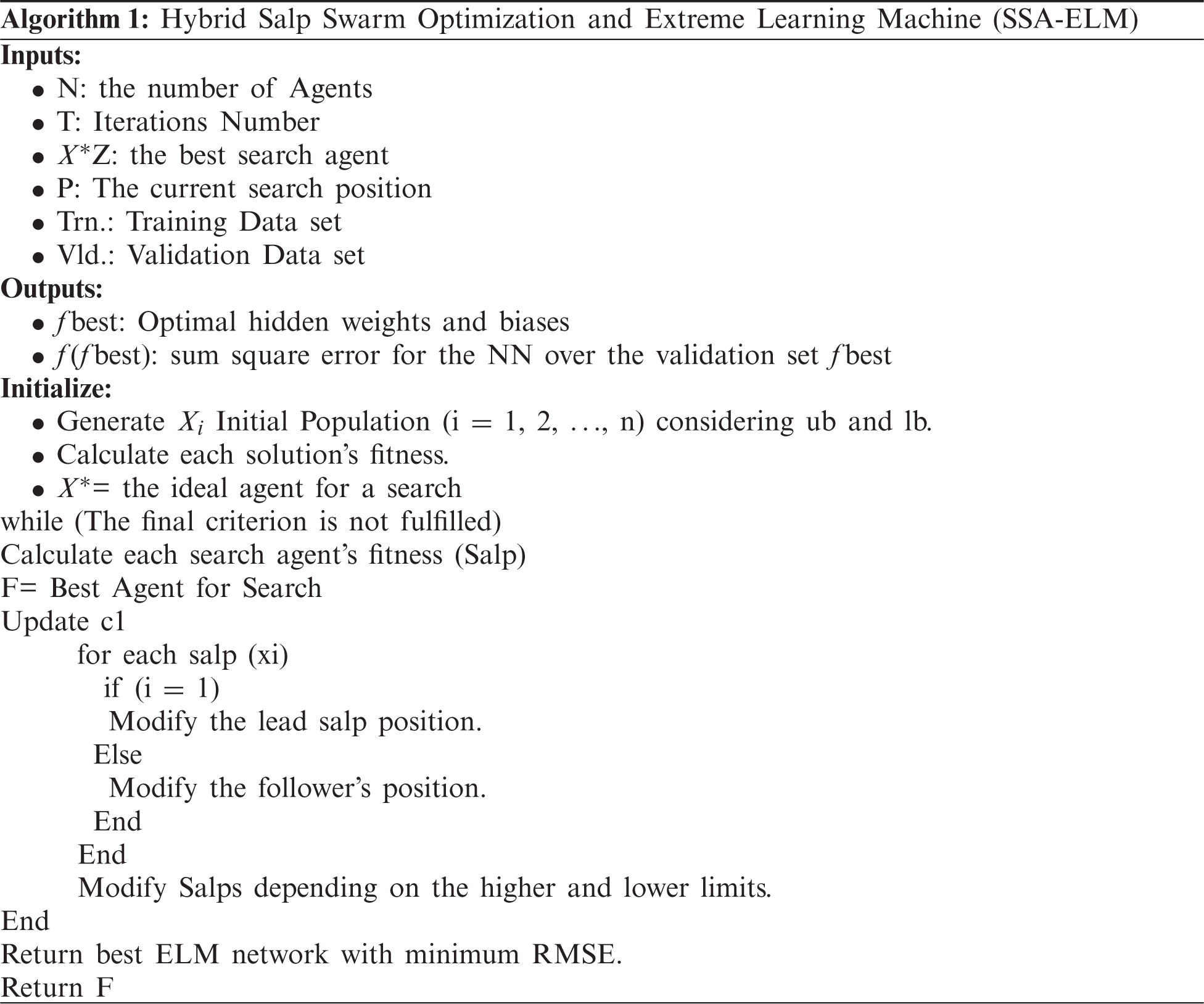
The hidden output layer matrix’ pseudo reverse matrix serves to establish the weight of the output layer matrix of an ELM and over-fit a significant amount of hidden layer nodes. In addition, the weight and hidden offset layer value of the ELM are randomly generated, resulting in multiple weights matrices of the output layer. The Salp Swarm Algorithm optimizes input weight and hidden layer bias values in the ELM to avoid confusion created by random selection of the two. Hence, iterative update and optimization [32] offered the globally best approach.

According to the literature [33], this section addresses the nature and implementation of the SSA - ELM training Algorithm. The SSA is used for the optimization of the ELM network, which serves the ELM candidate network for any salp path. SSA is programmed to maintain the parameters of the network to be optimized, namely the weights of a connection between the input and the hidden level and the bias of the neurons in the hidden layer. As a result, the length of each salp can be determined with the formula L = I*N + N, where I denotes the number of input variables. Fig. 2 depicts the architecture of the SSA-structural ELM.

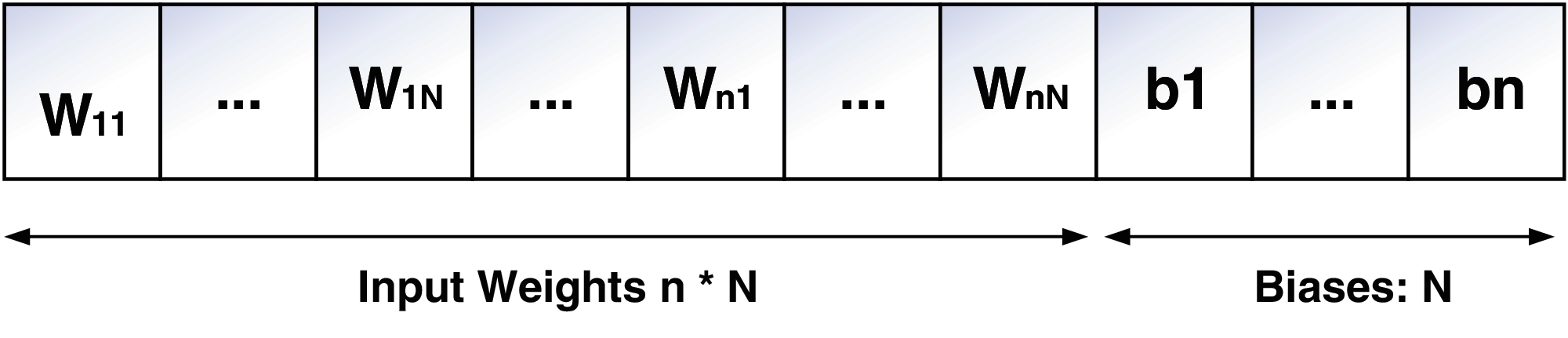
Figure 2: Structural design of SSA-ELM

4.2 GOA-ELM Model

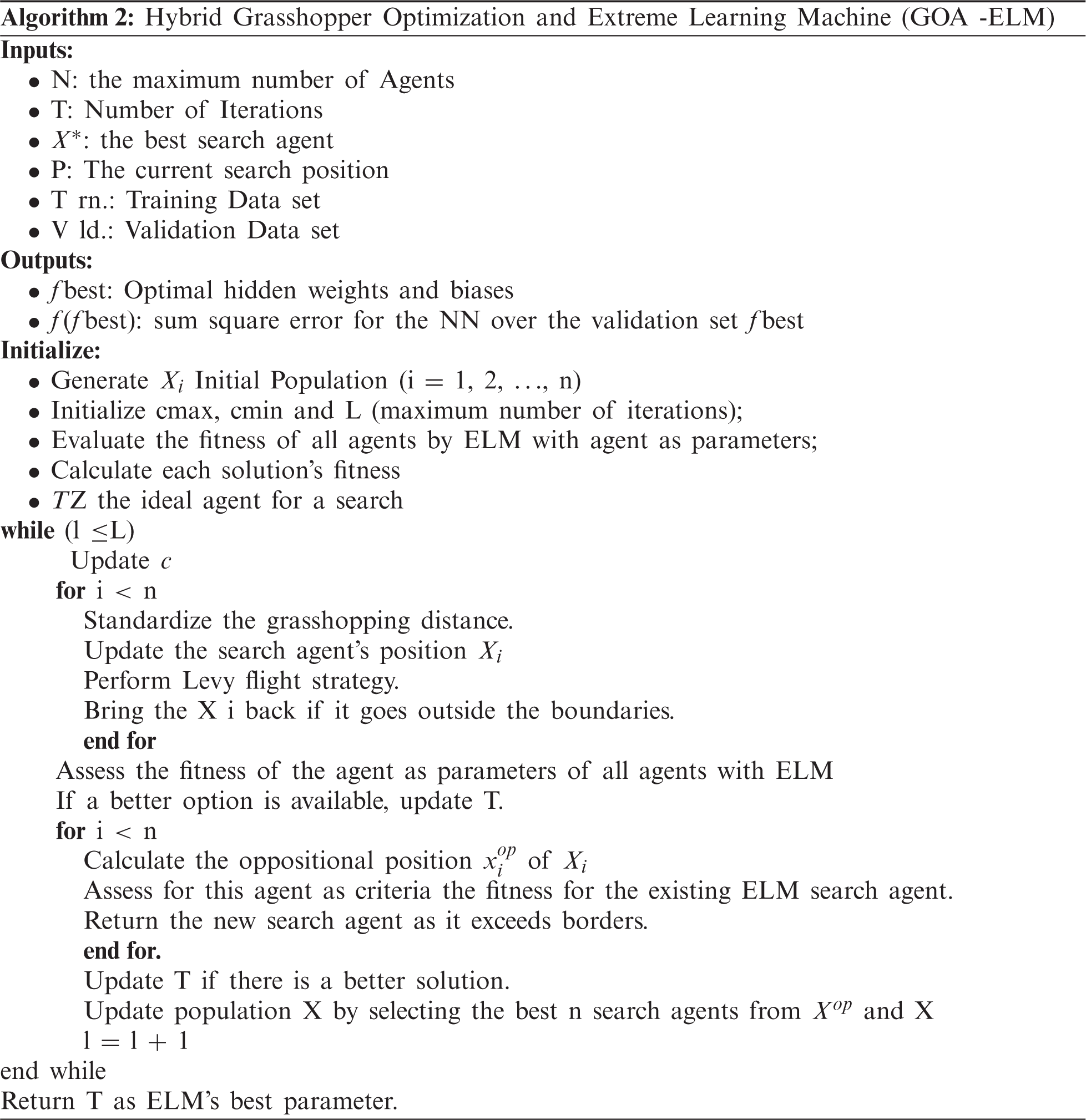
The hybrid ELM model based on GOA is mentioned in detail in this section. GOA is used in GOA-ELM to refine the parameters of ELM. The suggested technique is split into two sections. The first stage entails refining internal parameters. The second segment assesses the efficiency of the outer classification. The GOA technique dynamically adjusts the optimum parameters for the training set while tuning the inner parameters for ELM. The optimal parameters are then fed into the ELM model in the outer loop to perform the classification task.

4.3 GWO-ELM Model

This algorithm can be paired with other optimization algorithms to solve these issues and increase the performance of ELM. The ELM algorithm will be paired with GWO in this analysis since it has a sufficient convergence rate and does not have several tuning parameters. ELM, on the other hand, can be paired with other optimization algorithms. The following steps can be taken to build a hybrid ELM-GWO algorithm:

4.4 MFO-ELM Model

The proposed MFO-ELM model retains the same method for determining the output sheet's weights and preferences. The MFO algorithm is used to maximize the overall efficiency of the ELM by choosing the weights and expectations of the secret layer as described in Eq. (27). M variables must be calculated by the MFO, with M = (NH + 1) * NI where NH and NI are the total number of nodes in the secret and input layers, in that order. Individual vector ranges are limited to [−1, 1].

F(w)=∑j=1NValidation⁡∑i=1No⁡|Oij−dij|(27)

where NValidation is the number of data points in the validation set, No is the number of nodes in the output layer. Oij is the actual output on node i as a result of applying sample j to the ELM, and dij is the desired output on node i for a sample j.

Algorithm 4 presents an algorithm that depicts the proposed MFO-ELM model as follows:

4.5 WOA-ELM Model

The suggested WOA-ELM algorithm consists of the following steps:

1- Initialize all the humpback whales (z = 1, .., Ps) randomly where each whale represents a set of input weights and hidden biases within a range [−1, 1] as represented in Eq. (28)

sz=[w11h,….,w1lh,wnh1h,…,wnhlh,b1,b2,….,bnh] (28)

2- Evaluate the output weights and fitness of each whale and find sbestof all the solutions in the population. The fitness is defined as represented in Eq. (29)

f(sbest)=∑j=1Nv⁡||∑i=1nh⁡wio∅(wih.xj+bi)−tj||22Nv(29)

where, Nv indicates the number of validation samples

3- For each whale, calculate a, A, ζ, q, and pr. Update the position based on Eq. (24) and generate the new population.

4- Bound the new solutions using the following Eq. (30).

sz(k+1)={−1,sz(k+1)<−1,+1,sz(k+1)>+1(30)

and find the best new solution sbestnew.

5- Update the sbest using the norm of the output weights and the fitness value as (31).

sbest={sbestnew,if(|f(sbest)−f(sbestnew)|<εf(sbest) and wsbestnewo)sbest,otherwise} (31)

where f(sbest) and f(sbestnew) denotes the fitness of the best solution so far and the new best solution respectively. wsbesto and wsbestnewo represents the output weights of best solution so far and the best new solution respectively. ϵ > 0 is a user-defined tolerance rate.

6- Repeat steps 3–5 before the end condition is not met (i.e., the full number of iterations) to achieve the desired input weights and latent biases.

5  Experimental Results

5.1 Dataset Description

With the classification and predication information package of the UCI Machine Learning store used in the experiments and comparisons. Several highlights and incidents were chosen to provide the set of information as agents with various kinds of issues to be addressed in the strategy illustrated. To ensure that optimization algorithms are applied in colossal search spaces as seen in Tabs. 1 and 2, we picked a set of high-dimensional results separately.

We worked on two datasets, one for classification and the other for prediction.

5.1.1 Classification Dataset

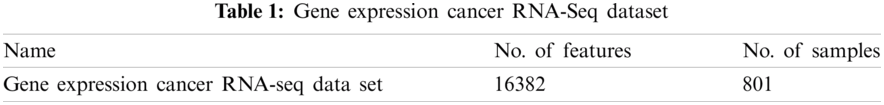
Cancer is one of the most dreaded and violent illnesses in the world, causing over 9 million deaths. The earlier the level of cancer is, the better the chance of survival. The RNA sequence analysis is one of the steps [34]. There has been an interest in human genomics research recently in developing reliability and precision of artificial intelligence approaches and optimization algorithms. Centered on tumor RNA sequence (RNA-Seq) gene expression data, the authors present five hybrid models for classifying different forms of cancer. This study will focus on KIRC “kidney renal clear cell carcinoma”, BRCA “breast invasive carcinoma”, LUSC “lung squamous cell carcinoma”, LUAD “lung adenocarcinoma”, and UCEC “uterine corpus endometrial carcinoma”. And the Description of the dataset will be illustrated in Tab. 1.

5.1.2 Predication Dataset

With the proliferation of smart energy meters and the widespread deployment of electricity generation technologies such as solar panels, there is a wealth of data on electricity demand available [35].

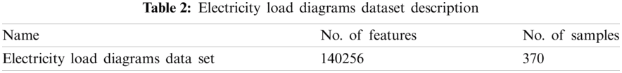
This information is a multivariate time series of power-related variables that can be used to predict and estimate potential energy demand. This paper presents five hybrid models for predicting the household power consumption dataset, which explains energy demand for a single house over a four-year period, And the Description of the dataset will be illustrated in Tab. 2.

5.2 Parameters Settings

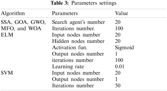
For the proposed and compared versions, 500 cycles have been planned. The ELM has 20 input layer nodes. It has twenty hidden nodes, but more hidden nodes are expected than algorithms of classical inclination. In the output layer, it has one node. The SSA, GOA, GWO, MFO and ELM algorithms parameter settings are summarized in the Tab. 3.

5.3 Simulation Results

The following Results have been run on Google Colab, The VM used for Collaboratory appears to have 2-core Xeon 2.2GHz, 13GB RAM and 2 vCPU when checking using psutil (so a n1-highmem-2 instance)

5.3.1 Classification Results

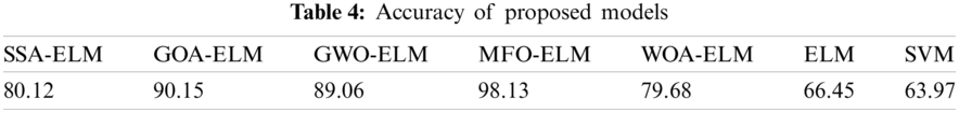
The hybrid MFO-ELM model has a better accuracy than SSA-ELM, GOA-ELM GWO-ELM, WOA-ELM, standard ELM and SVM as shown.

1- Accuracy

MFO-ELM has a better Accuracy than other Algorithms as shown in Tab. 4.

2- Learning Curves

All proposed models converged to global minimum after few iterations as shown in Figures from Figs. 3–7.

3- Confusion Matrix

SSA-ELM has misclassified Class “COAD” between Class (COAD and BRCA) as shown in Fig. 8. GOA-ELM has misclassified Class “COAD” as shown in Fig. 9. GWO-ELM has misclassified Class “COAD” as shown in Fig. 10. MFO-ELM has misclassified Class “PRAD” as shown in Fig. 11. WOA -ELM has classified all classes correctly as shown in Fig. 12. ELM has misclassified Class “COAD, KIRC” as shown in Fig. 13.

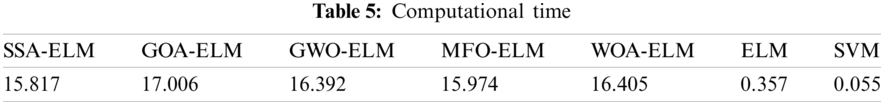
4- Computational Time

Instead of the better accuracy if MFO- ELM, SVM has the best Computational Time, As shown in Tab. 5, the time is calculated in Seconds

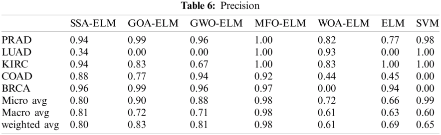
5- Precision

MFO- ELM has the best Precision across all classes as shown below in Tab. 6.

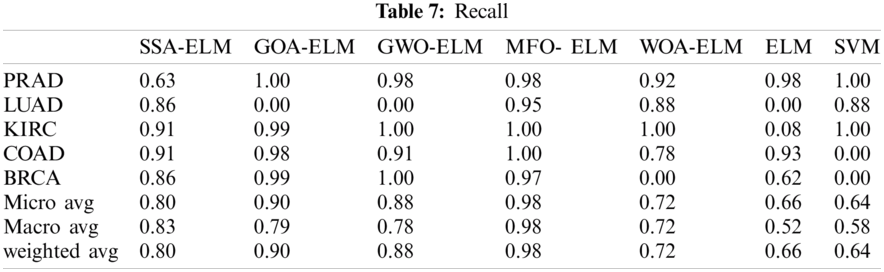
6-Recall

MFO- ELM has the best Recall across all classes as shown below in Tab. 7.

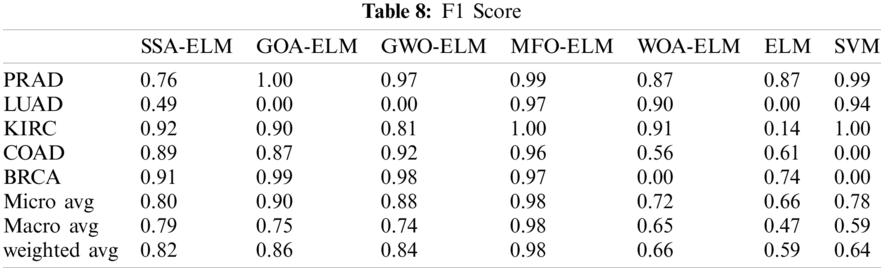
7- F1 Score

MFO- ELM has the best F1Score across all classes as shown below in Tab. 8.

5.3.2 Predication Results

The hybrid GOA-ELM model has a better accuracy than SSA-ELM, MFO-ELM GWO-ELM, WOA-ELM, standard ELM and SVM as shown.

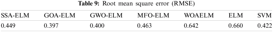
1- Root Mean Square Error (RMSE):

GOA-ELM has the least Mean Squared Error as shown in Tab. 9.

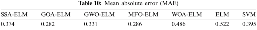
2- Mean Absolute Error (MAE):

GOA-ELM has the least Mean Absolute Error as illustrated in Tab. 10.

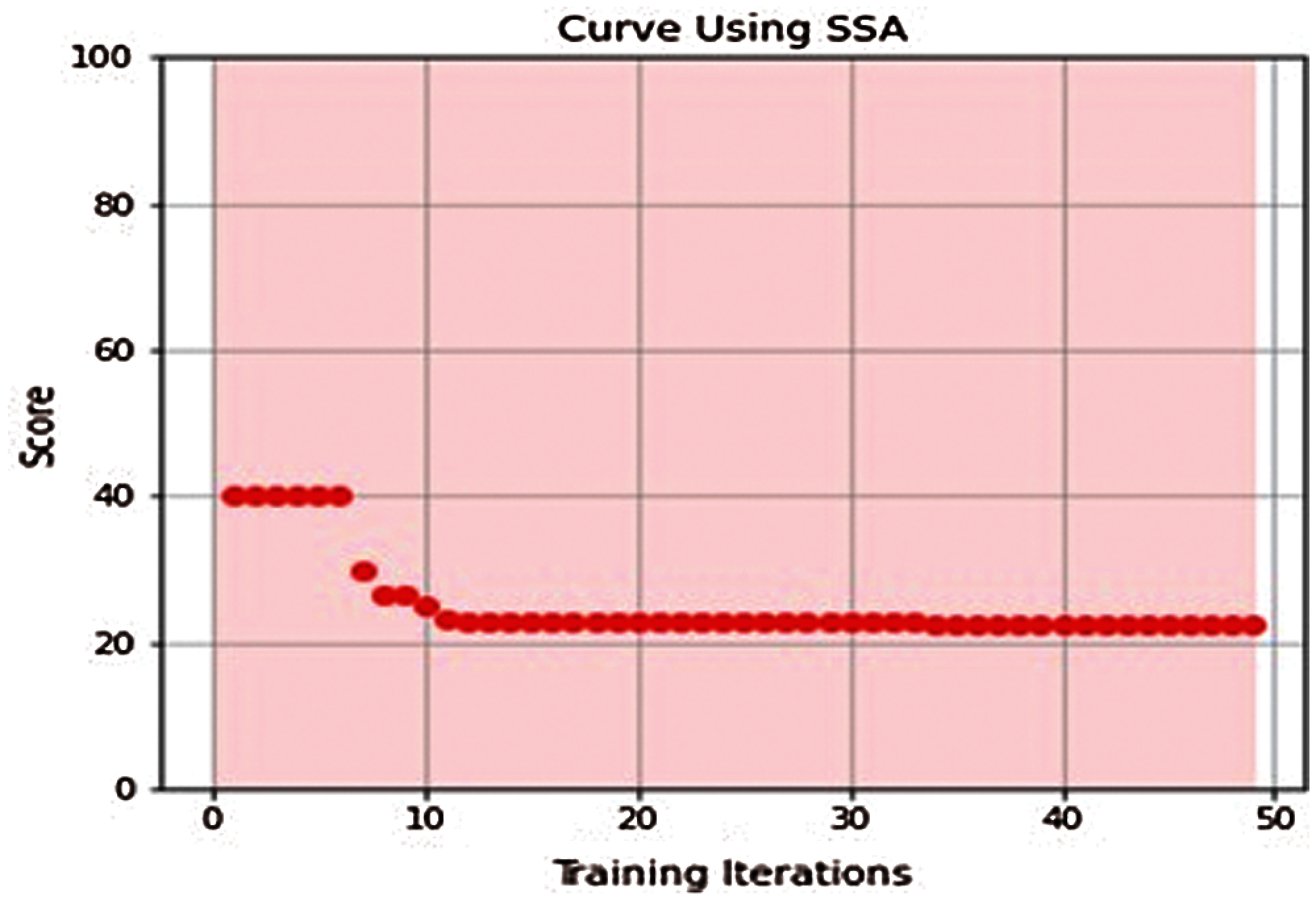
Figure 3: SSA-ELM learning curve

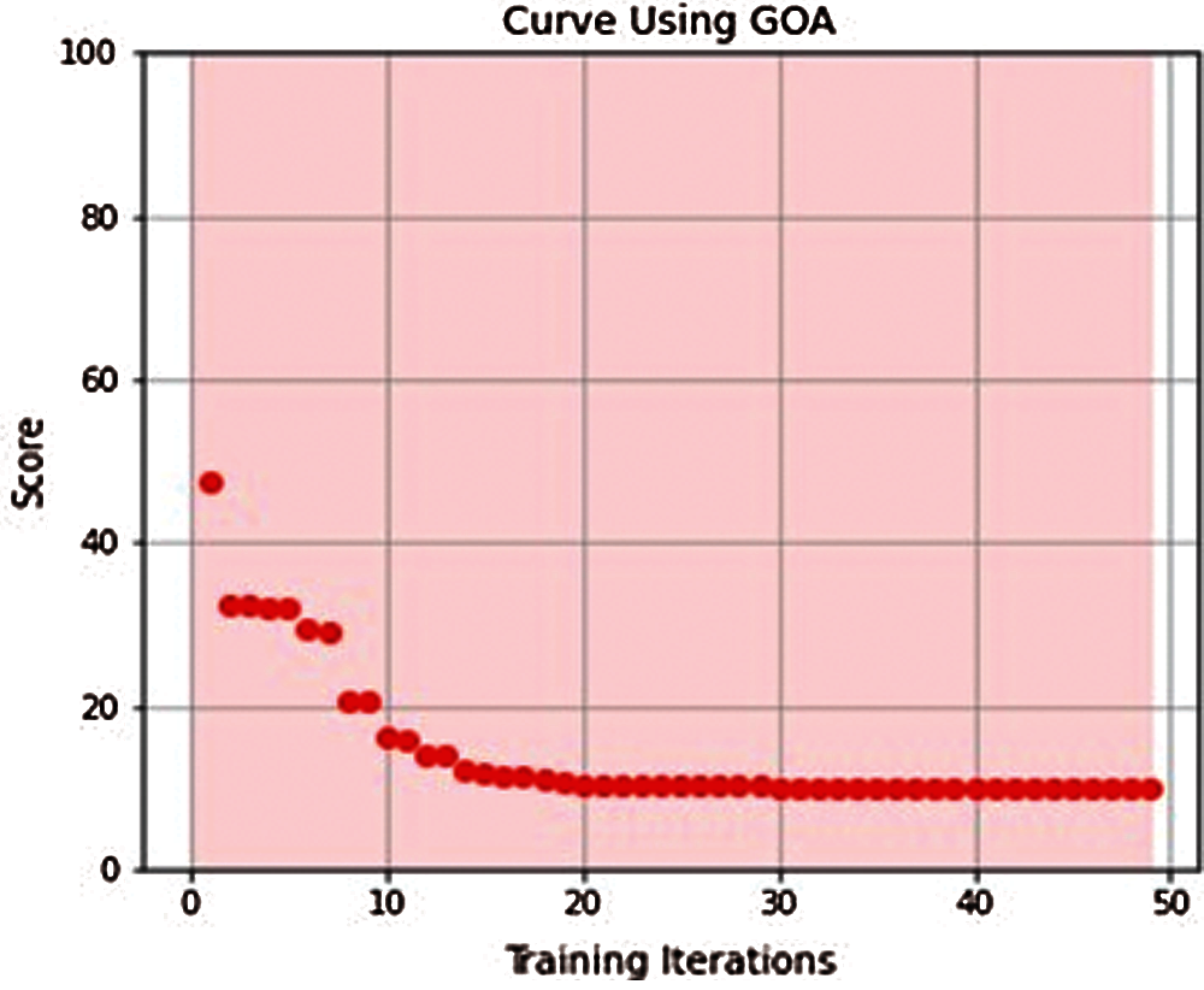
Figure 4: GOA-ELM learning curve

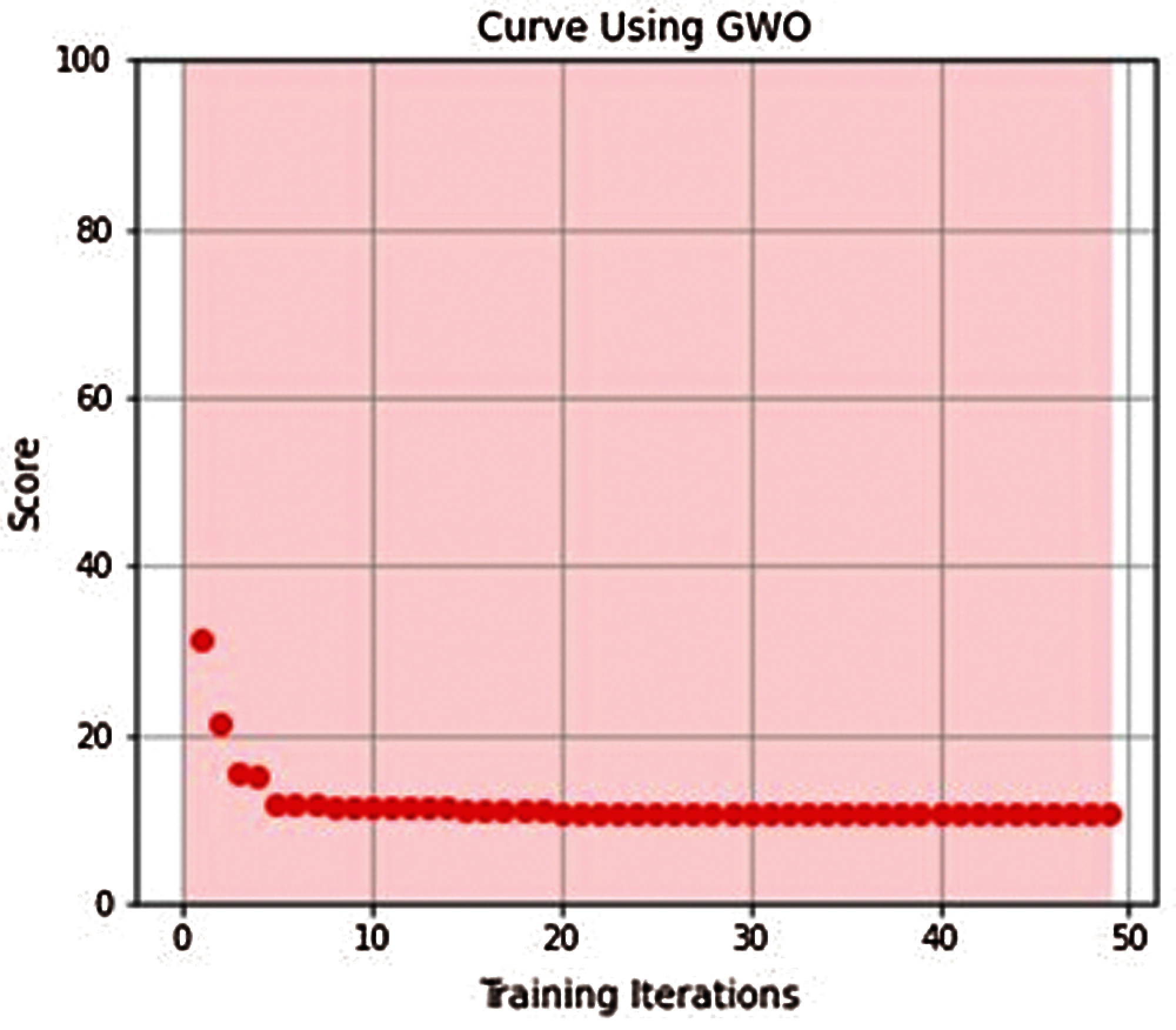
Figure 5: GWO_ELM learning curve

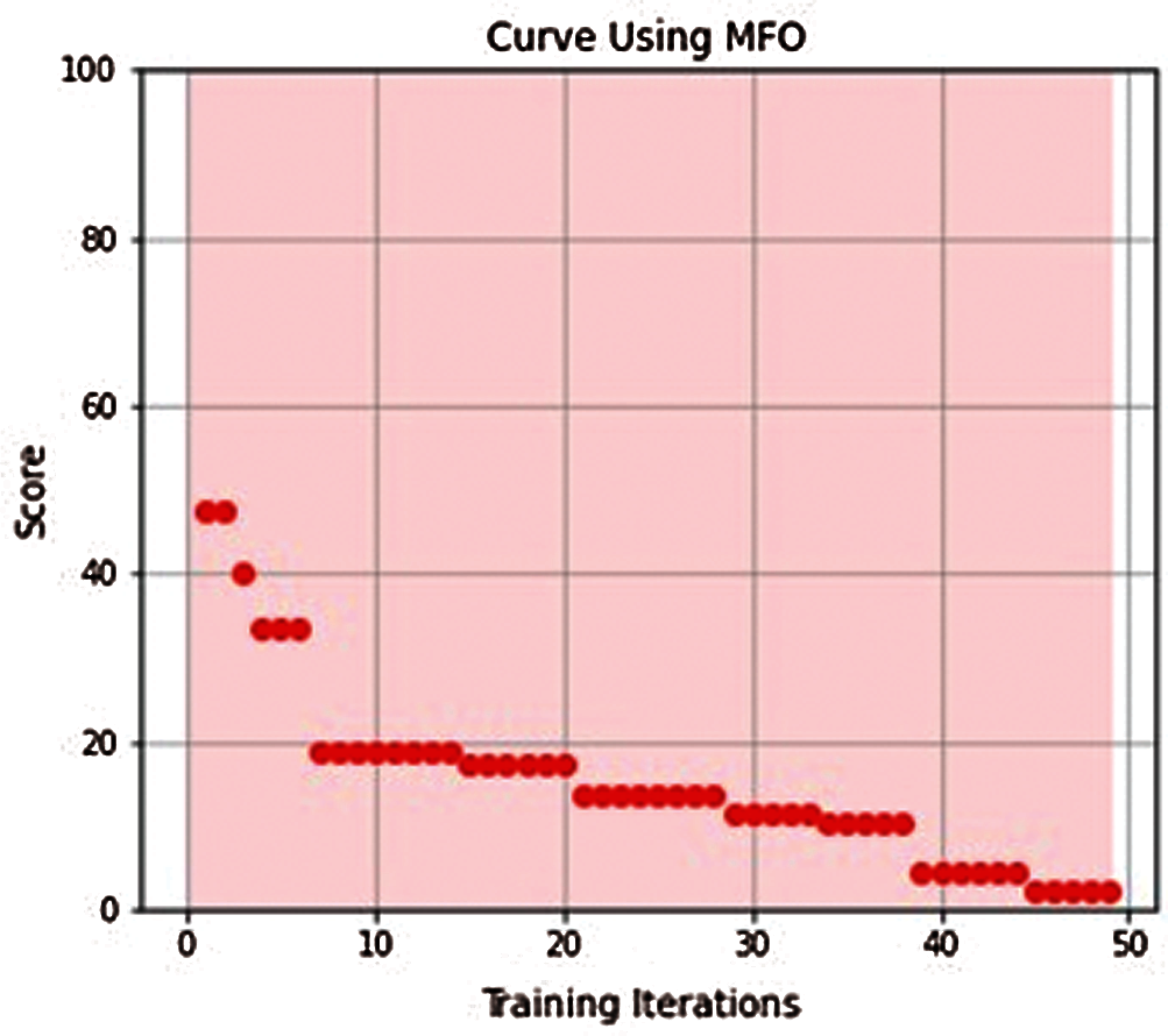
Figure 6: MFO-ELM learning curve

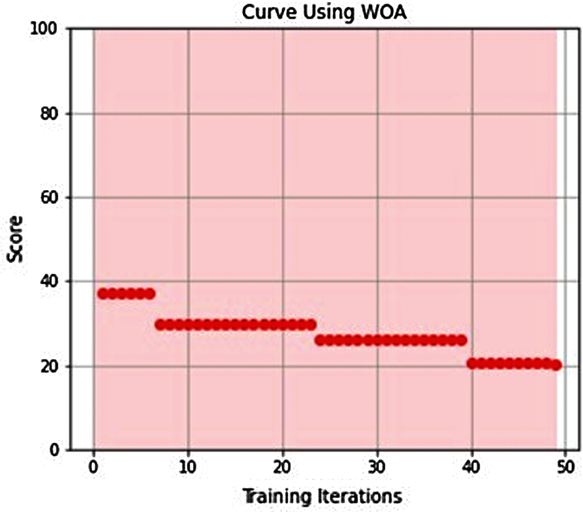
Figure 7: WOA-ELM learning curve

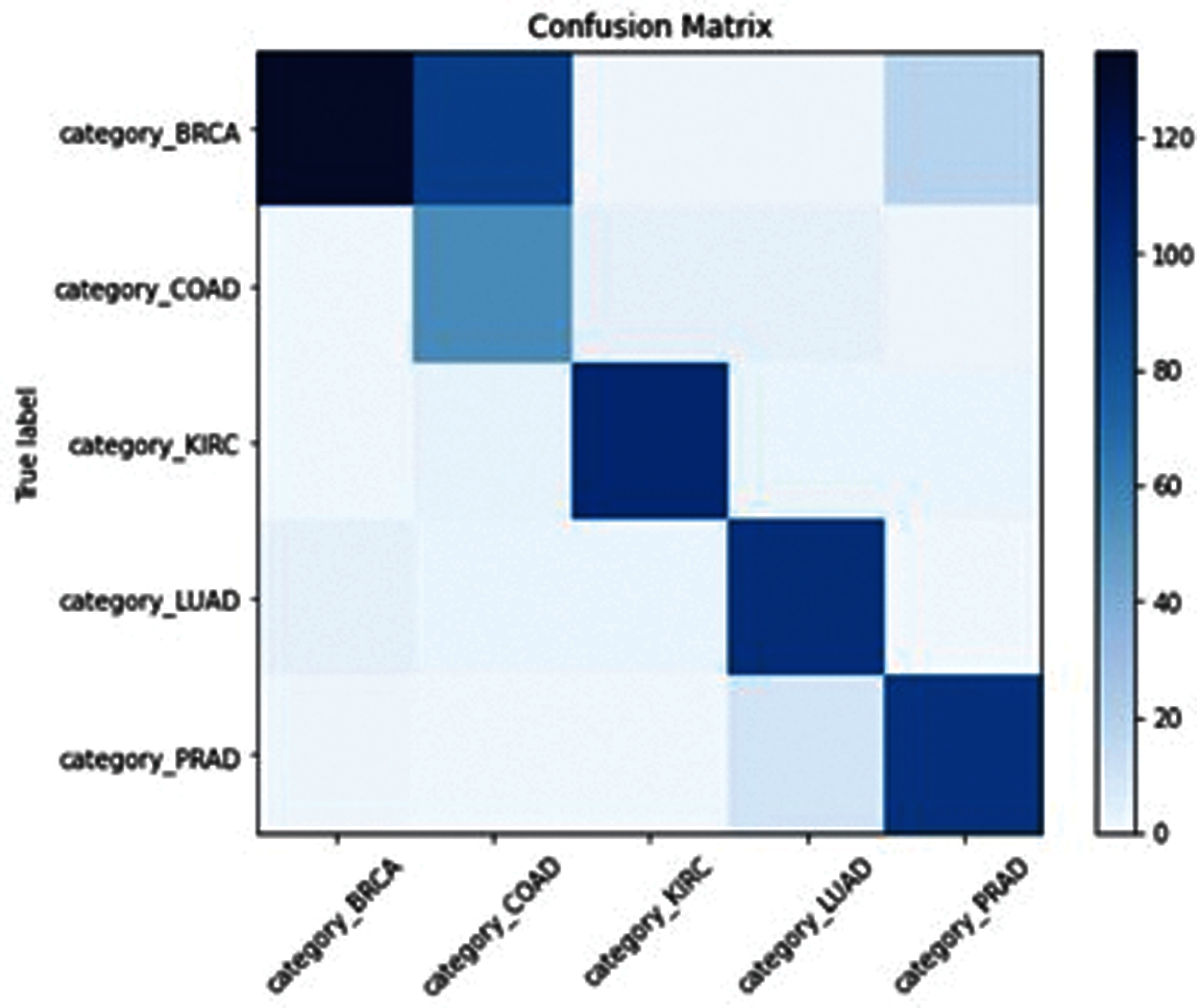
Figure 8: SSA-ELM confusion matrix

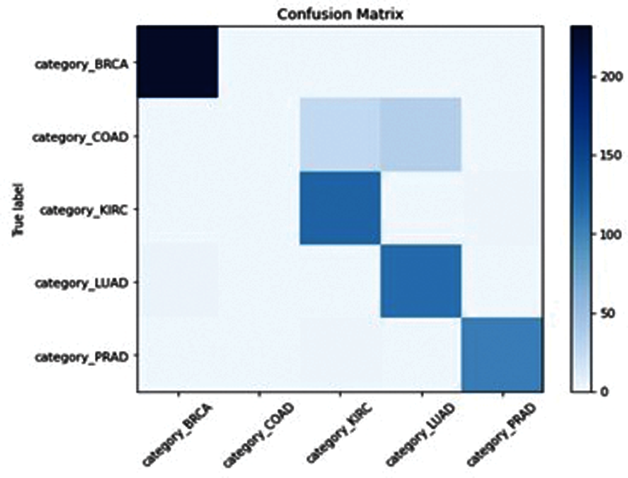
Figure 9: GOA-ELM confusion matrix

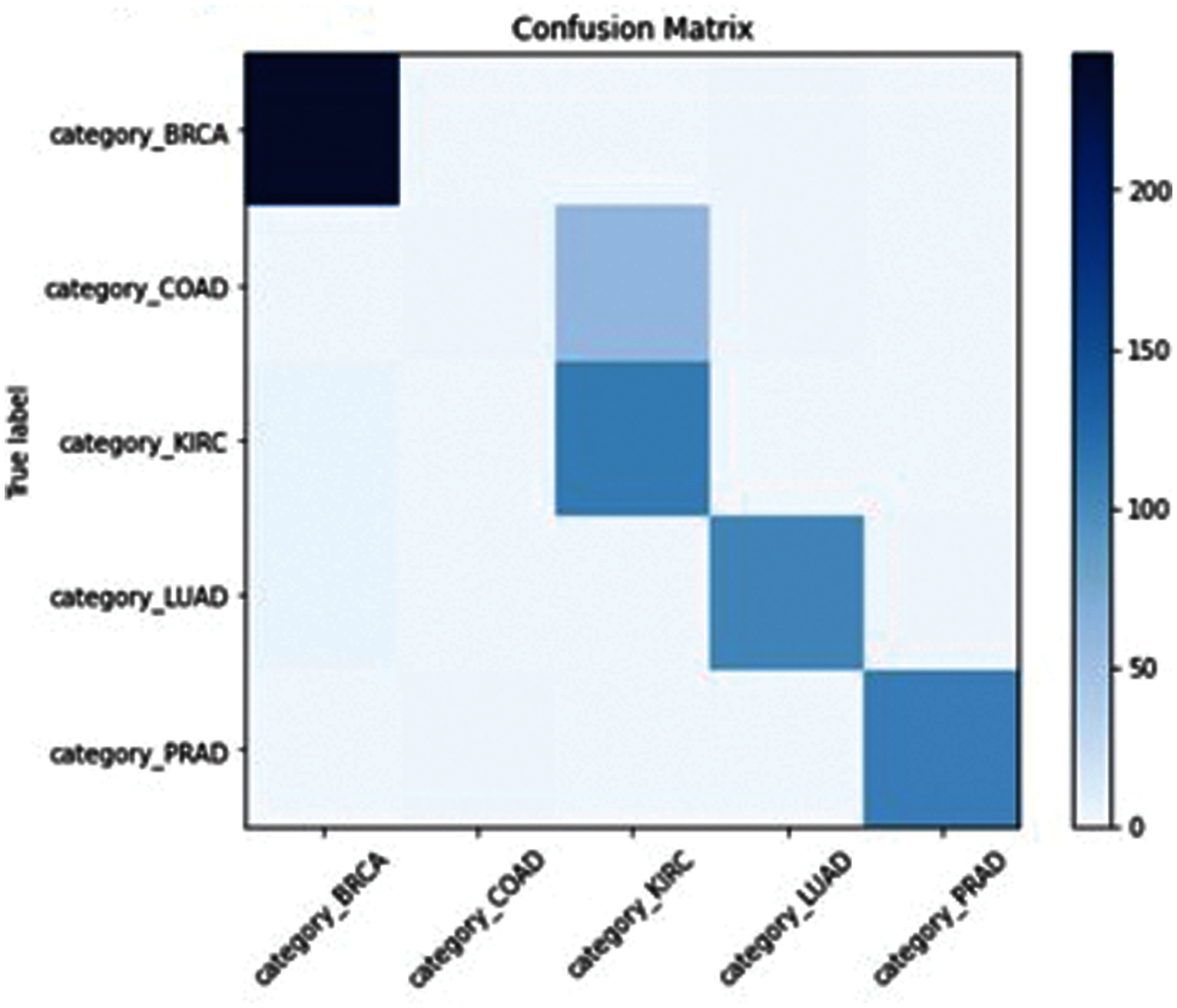
Figure 10: GWO-ELM confusion matrix

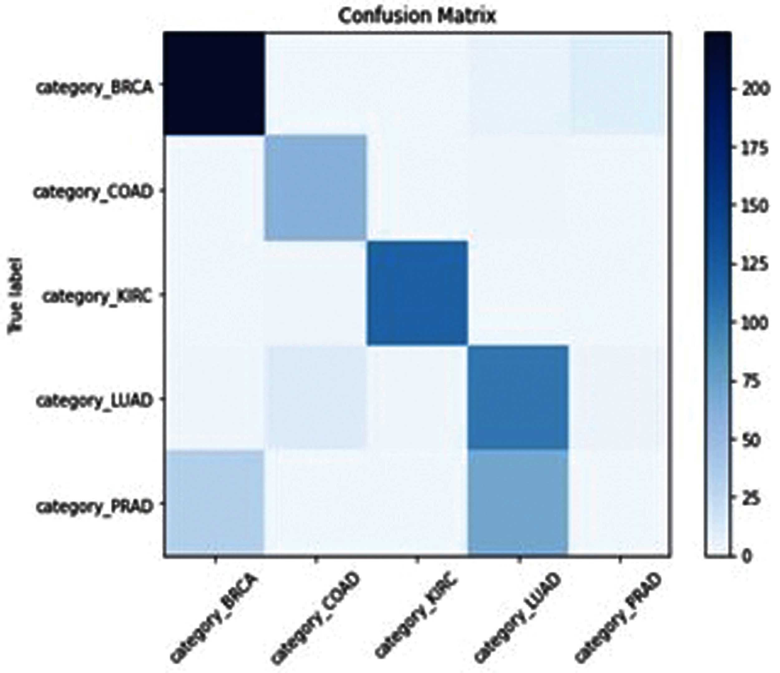
Figure 11: MFO-ELM confusion matrix

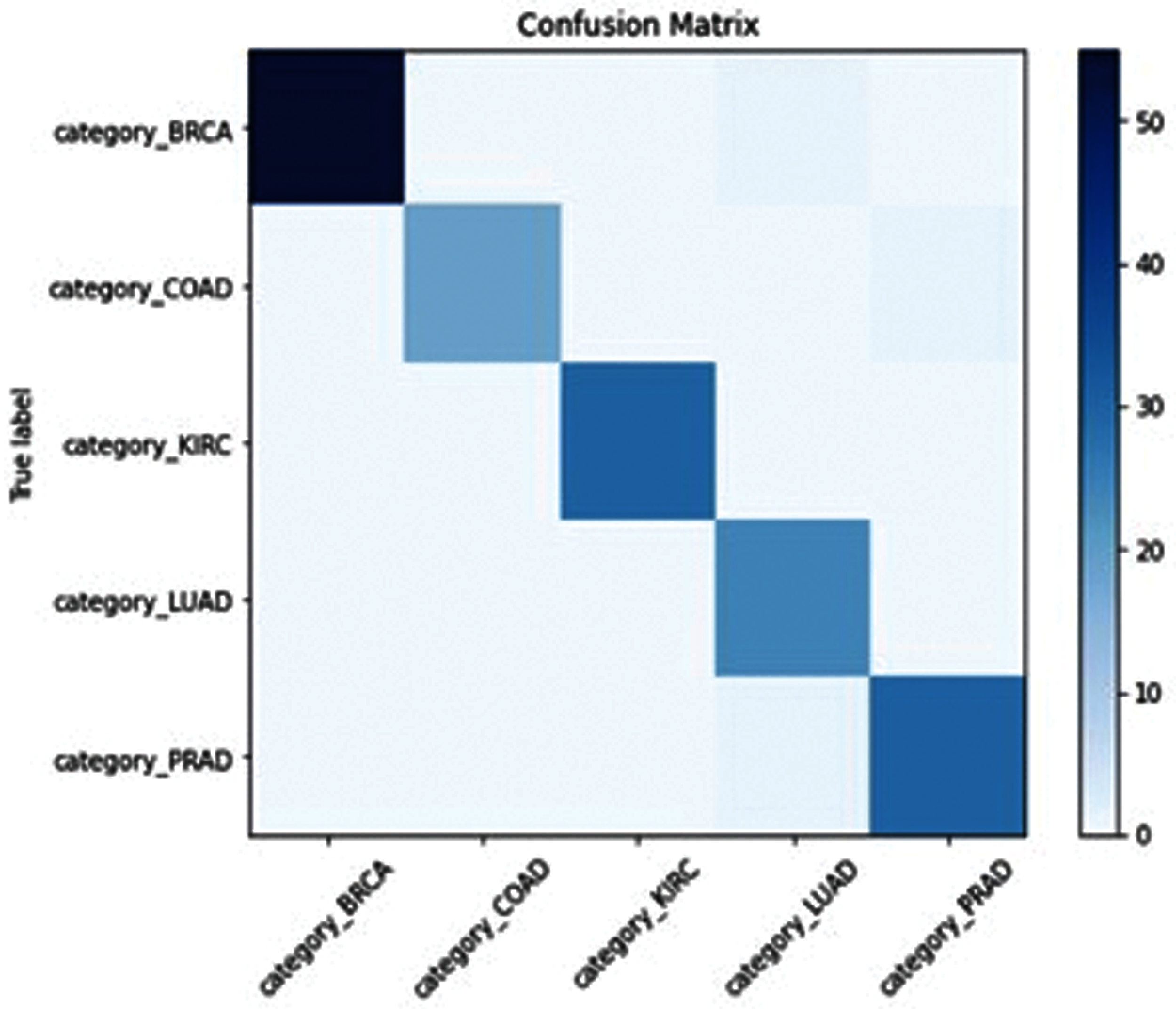
Figure 12: WOA-ELM confusion matrix

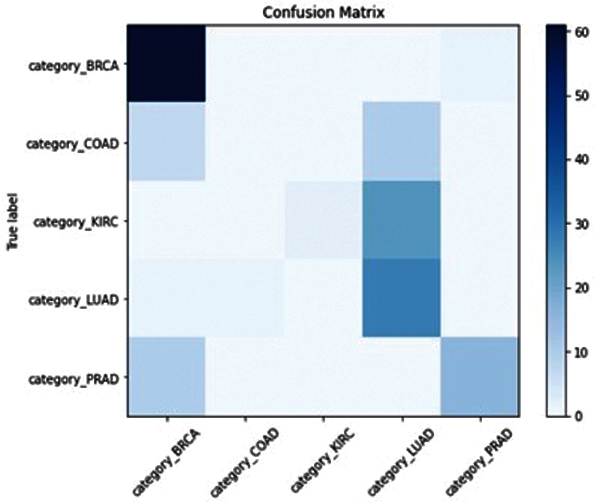
Figure 13: ELM confusion matrix

6  Conclusions and Future Work

This paper proposes five hybrid models for enhancing ELM efficiency. The proposed hybrid algorithms are namely, “Salp Swarm Algorithm (SSA-ELM), Grasshopper Algorithm (GOA-ELM), Grey Wolf Algorithm (GWO-ELM), Whale optimization Algorithm (WOA-ELM) and Moth Flame Optimization (MFO-ELM). Experimental results for gene classification dataset showed that MFO achieved best accuracy and efficiently select weights and hidden layer biases of ELM. The proposed models addressed the over-fitting issue that afflicted the regular ELM model. The five hybrid models had been used for predicting the household power consumption dataset, which explains energy demand for a single house over a four-year period. The proposed GOA-ELM model has achieved the best result in predicting and estimating potential energy demand.

In Future work, New Hybrid models will be developed. in addition, we will try to test the hybrid models on more datasets in different fields and check the efficiency of each algorithm in each dataset and which fits each field. And we are going to try these models on Higher datasets with millions of features.

Funding Statement: The authors received no specific funding for this study.

Conflicts of Interest: The authors declare that they have no conflicts of interest to report regarding the present study.

This work is licensed under a Creative Commons Attribution 4.0 International License, which permits unrestricted use, distribution, and reproduction in any medium, provided the original work is properly cited.