Computers, Materials & Continua DOI:10.32604/cmc.2022.020732
Article

Analysis of Pneumonia Model via Efficient Computing Techniques

Kamaledin Abodayeh1, Ali Raza2,3,*, Muhammad Rafiq4, Muhammad Shoaib Arif5, Muhammad Naveed5, Zunir Zeb3, Syed Zaheer Abbas3, Kiran Shahzadi3, Sana Sarwar3, Qasim Naveed3, Badar Ul Zaman3 and Muhammad Mohsin6

1Department of Mathematics and General Sciences, Prince Sultan University Riyadh, 66833, Saudi Arabia
2Department of Mathematics, Govt. Maulana Zafar Ali Khan Graduate College Wazirabad, 52000, Punjab Higher Education Department (PHED), Lahore, 54000, Pakistan
3Department of Mathematics, National College of Business Administration and Economics Lahore, 54660, Pakistan
4Department of Mathematics, Faculty of Sciences, University of Central Punjab, Lahore, 54500, Pakistan
5Department of Mathematics, Air University, Islamabad, 44000, Pakistan
6Department of Mathematics, Technische Universitat Chemnitz, 62 09111, Germany
*Corresponding Author: Ali Raza. Email: Alimustasamcheema@gmail.com
Received: 06 June 2021; Accepted: 20 August 2021

Abstract: Pneumonia is a highly transmissible disease in children. According to the World Health Organization (WHO), the most affected regions include south Asia and sub-Saharan Africa. Worldwide, 15% of pediatric deaths can be attributed to pneumonia. Computing techniques have a significant role in science, engineering, and many other fields. In this study, we focused on the efficiency of numerical techniques via computer programs. We studied the dynamics of the pneumonia-like infections of epidemic models using numerical techniques. We discuss two types of analysis: dynamical and numerical. The dynamical analysis included positivity, boundedness, local stability, reproduction number, and equilibria of the model. We also discuss well-known computing techniques including Euler, Runge Kutta, and non-standard finite difference (NSFD) for the model. The non-standard finite difference (NSFD) technique shows convergence to the true equilibrium points of the model for any time step size. However, Euler and Runge Kutta do not work well over large time intervals. Computing techniques are the suitable tool for cross-checking the theoretical analysis of the model.

Keywords: Pneumonia disease; epidemic model; computing techniques; convergence analysis

1  Introduction

Pneumonia is a disease of the lungs that can cause minor to severe illness in people of different ages. The swelling of the lungs that occurs during pneumonia is most commonly caused by infection with bacteria or molds. There are also a few noninfectious types of pneumonia. These are caused by inhaling contaminated materials into the lungs. Most pneumococcal poisons are insignificant, but some of them are harmful, causing such issues as brain damage and hearing problems. Meningitis is the most severe disease caused by pneumococcal pneumonia, and it is more common in children who are less than five years old and it can cause long-term disease in individuals over 50 years old. Bacteria are a main and major cause of pneumococcal disease and blood-borne infection. About 1% of children under five years old with this infection die. The chance of death from pneumococcal pneumonia is also higher among the elderly. About 5% of people with pneumonia die, but the ratio is higher among the elderly. Pneumococcal pneumonia can be asymptomatic if there are no bacteria or cold weather during that period. Pneumococcal pneumonia can cause swelling of the throat, necessitating ear tubes in some children. Symptoms of pneumococcal pneumonia can include greenish, yellow, or bloody liquid produced during coughing, weakness, profuse sweating, difficulty breathing, severe headache, and severe chest pain. Symptoms tend to worsen when the patient is hungry or exhausted. In 2014, Mochan et al. [1] dynamically described the interhost immune response to bacterial pneumonia infection in murine strains in a simple ordinary differential equation model. In 2014, Drusano et al. [2] reported the effects of granulocytes in the eradication of bacterial pathogens, and there was no antimicrobial therapy involved in this work. In 2015, Ndelwa et al. [3] produced a dynamic mathematical model for the transmission of pneumonia with screening and medication and analyzed it to assess transmission and effects. In 2015, Kosasih et al. [4] analyzed a mathematical model of cough sounds using wavelet-based crackle detection work for rapid diagnosis of bacterial pneumonia in children. In 2016, Cesar et al. [5] mathematically estimated fine particulate matter in a model and evaluated medications for pneumonia and asthma among children. In 2016, Marchello et al. [6] listed atypical bacterial pathogens as the main causes of such lower respiratory diseases as coughs, bronchitis, and CAP. In 2017, Cheng et al. mathematically and dynamically evaluated an IAV-SP model. A quantitative risk-assessment framework was established to improve respiratory health due to COPD [7]. In 2017, Kosasih et al. [8] provided a simple mathematical model showing the analysis of measurements for clinical diagnosis of pneumonia among children. In 2017, Tilahun et al. proposed a deterministic nonlinear mathematical model and analyzed optical control strategies for bacterial pneumonia. Results are shown graphically [9]. In 2018, Raj et al. [10] analyzed the classification of asthma and pneumonia based upon mathematical features of cough sounds among poorer segments of the population. In 2018, Kizito et al. presented a mathematical model that shows the control of pneumonia spread by bacteria. It also gave the dynamics of treatment and formulation of vaccines [11]. In 2018, Mbabazi et al. [12] investigated a nonlinear mathematical model that modeled intra-host co-infection influenza A virus and pneumonia. In 2018, Tilahun et al. [13] proposed a co-infection model for pneumonia-typhoid and mathematically analyzed their characteristic relationship for the development of medical strategies. In 2019, Tilahun et al. described a model of pneumonia-meningitis co-infection with the help of ordinary differential equations and theorems. It explained different techniques for disease clearance [14]. In 2020, Naveed et al. [15] reported a dynamic analysis of coronavirus while assessing the sensitivity of model parameters. In 2019, Kosasih et al. [16] explained the main cause of pneumonia affecting children in early childhood in poor regions of the world. In 2019, Tilahun et al. [17] analyzed a co-infection mathematical model for the bacterial disease of pneumonia and meningitis. In 2019, Mbabazi et al. [18] proposed a mathematical model of pneumococcal pneumonia with time delays and performed Hopf-bifurcation analysis. In 2020, Otoo et al. [19] analyzed a model of pneumonia spread by bacteria. The analysis determined the effects of vaccination on control of this disease. In 2020, Zephaniah et al. [20] presented the dynamics of a mathematical model of pneumonia, showing the result graphically. In 2019, Raza et al. [21] described the stochastic dynamics of gonorrhea-like infections. In 2020, Jung et al. [22] demonstrated the observations using different clinical tests and showed the cause of disease, a novel pathogen. Many mathematical models are studied with different techniques, as shown in previous works [23–27]. Well-known mathematical models can be investigated with the help of efficient techniques [28–39]. The rest of the paper is organized as follows. In Sections 2–4, we investigate the dynamic analysis of the model. Section 5 explains the well-known computer methods used on this model. The last two sections present the results, discussion, and conclusion.

2  Formulation of Pneumonia Model

For any arbitrary time t, the parameters and variables of pneumonia disease described as follows: S(t): represents the susceptible, who is at risk of acquiring infection pneumonia, C(t): represents the carrier individuals carrying the pneumonia bacteria and can transfer the infection, I(t) : represents the infective individuals that are capable of transmitting the infection to individuals at risk, R(t): represents the individuals who have been recovered after the treatment of Pneumonia, μ: represents the natural mortality rate of individuals per capita, Λ: represents the recruitment rate into susceptible population per capita, θ: represents the proportion of susceptible individuals who joins the carriers, σ: represents the disease induced mortality rate birth rate of human population per capita, β: represents the recovery rate of carriers per capita, α: represents the infection force of susceptible individuals, τ: represents the recovery rate of individuals who are infected of Pneumonia per capita, π: represents the rate of developing symptoms by carriers, η: represents the rate of treated individuals becoming susceptible, γ: represents the rate of susceptible individuals getting vaccinated,ω: represents the rate of treated individuals having vaccinated, ω: represents the coefficient of transmission for the carrier subgroup, δ: represents the rate of transmission, p: represents the probability that shows a contact is efficient enough to cause infection, k: represents the rate of contact. The governing equations of the model are as follows:

S′(t)=Λ−δI(t)S(t)N−δωS(t)C(t)N−μS(t)+ηR(t).(1)

C′(t)=δI(t)θS(t)N+δωC(t)θS(t)N−μC(t)−βC(t)−πC(t).(2)

I′(t)=δ(I+ωC(t))N(1−θ)S(t)2+πC(t)−(τ+μ+Φ)I(t).(3)

R′(t)=βC(t)+τI(t)−(μ+η)R(t).(4)

2.1 Fundamental Properties of Model

We consider all parameters positive and show that the solution is bounded in Ψ={(S,C,I,R)ϵℜ+4:0≤N≤Λμ}, N = S + C + I + R.

Lemma 1: The initial values {S(0),C(0),I(0),R(0)}∈Ψ,then the solution set {S(t),C(t),I(t),R(t)}is positive of all t≥0.

Proof: From Eq. (1), we have

dSdt=∧−δ(I+ωCN)S−μS+ηR

dSdt≥−(δ(I+ωCN)+μ)S

∫⁡dSS≥−∫⁡(δ(I+ωCN)+μ)dt

S=S(0)e−(δ(I+ωCN)+μ)≥0

So, S ≥0 similarly shows that for Eqs. (2)–(4)

Lemma 2: The solution of the model equation in (1–4) are bounded in Ψ for all t≥0.

Proof: Firstly, adding the Eqs. (1)–(4) as follows:

dNdt=Λ−μN−σI.

dNdt≤Λ−μN.

N≤Λμ+(N0−Λμ)e−μt.

where N0 is the initial condition of N,

So, limt→∞⁡SupN(t)≤Λμ. This show that 0≤N≤Λμ and N = S + C + I + R, then all variable is bounded in Ψ.

2.2 Steady States of Pneumonia Model

There are two steady states of Eqs. (1)–(4), as follows: disease-free equilibrium (DFE)=(S0,C0,I0,R0)=(Λμ,0,0,0), and endemic equilibrium (EE)=(S1,C1,I1,R1),

where

S1=NR0,C1=θΛKb(μ+η)(R0−1)R0[(Kb(Ka(μ+η)−ηθB))−ητ(Ka(1−θ)+πθ)]−σ(Ka(1−θ)+πθ)(μ+η)],

I1=Λ(Ka(1−θ)+πθ))(μ+η)(R0−1)R0[(Kb(Ka(μ+η)−ηθB))−ητ(Ka(1−θ)+πθ)]−σ(Ka(1−θ)+πθ)(μ+η)],

R1=(βθKb+τ(Ka(1−θ)+πθ))Λ(R0−1)R0[(Kb(Ka(μ+η)−ηθB))−ητ(Ka(1−θ)+πθ)]−σ(Ka(1−θ)+πθ)(μ+η)].

3  Reproduction Number of Pneumonia Model

The next-generation matrix method is presented for the system (1–4). We calculate two types of matrices like transmission and transition after assuming the disease-free equilibrium as follows:

A=[δωθδθδω(1−θ)δ(1−θ)],B=[Ka0−πKb]

AB−1=[δθ(ωKb+π)KaKbδθKaKaKbδ(1−θ)(ωKb+π)KaKbδKa(1−θ)KaKb]

where Ka=(μ+β+π), Kb=τ+μ+σ.

|AB−1−λI|=|δθ(ωKb+π)KaKb−λδKaθKaKbδ(1−θ)(ωK2+π)KaKbδK1(1−θ)KaKb−λ|=0.

(δθ(ωKb+π)KaKb−λ)(δKa(1−θ)KaKb−λ)−(δKaθKaKb)(δ(1−θ)(ωKb+π)KaKb)=0

λ=δ[Ka(1−θ)+θ(wKb+π)]KaKb.

The spectral radius of the model is denoted by R0=δ[Ka(1−θ)+θ(wKb+π)]KaKb.

4  Local Stability

Theorem: The disease-free equilibrium of model (1–4) is locally asymptotically stable if the reproduction number is less than one and unstable if it is greater than one.

Proof: To prove the local asymptotically stable disease-free equilibrium, we take the Jacobian matrix of SCIR Model of pneumonia model at disease-free equilibrium. To show that trace is less than zero and a determinant greater than zero.

J(S0,C0,I0,R0)=[−μ00η0−Ka000π−Kb00βτ−(μ+η)].

where, Ka=(μ+β+π), Kb = τ+μ+σ.

trace(J)=−μ−Ka−Kb−(μ+η)=−(2μ+Ka+Kb+η)⟨0,det(J)=−μ(−KaKb(μ+η))⟩0.

where −(2μ+Ka+Kb+η<0).

Be not be negative and δ[Ka(1−θ)+θ(ωKb+π)] is positive and also KaKb>0and we note that determinant (J) also positive, which is −μ(−KaKb(μ+η)) > 0, thus we have

R0=δ[Ka(1−θ)+θ(ωKb+π)]KaKb<1.

The above discussion is about the matrix J, a trace is less than zero and a determinant greater than zero. So, the disease-free equilibrium point is locally asymptotically stable if R0<1.

Theorem: If the reproduction number is greater than one, then the endemic equilibrium of the model Eqs. (1)–(4) is locally asymptotically stable in Ψ.

Proof: The Jacobian matrix at endemic equilibrium is as follows:

J(S1,C1,I1,R1)=[−(α1+μ)00ηα1θ−Ka00α1(1−θ)π−Kb00βτ−(μ+η)]

where Ka=(μ+β+π), Kb = τ+μ+σ.

P(λ)=|λI−J(S1,C1,I1,R1)|=|−(α1+μ)00ηα1θ−Ka00α1(1−θ)π−Kb00βτ−(μ+η)|=0

P(λ)=λ4+c1λ3+c2λ2+c3λ+c4

where c1=2μ+η+Ka+Kb+α1, c2=(η+μ)(Ka+Kb+α1+μ)+KaKb+(α1+μ)(Ka+Kb), c3=KaKb(η+μ)+(Ka+Kb)(α1+μ)(η+μ)+KaKb(α1+μ)+ητα1(1−θ)+ηβθα1, c4=KaKb(α1+μ)(η+μ)+ηα1τθπ+ηKaα1τ(1−θ)+α1Kaηβθ.

By using Routh Hurwitz method for order 4th as follows:

[1c1c2−(c3/c1)c2c4λ4c30λ3c40λ2c3−(c1c4/(c2−(c3/c1)))c100λ001]

The endemic equilibrium is locally asymptotically stable for the reproduction number greater than one if

c1>0,c2−(c3c1)>0c3−(c1c4(c2−(c3c1)))>0c4>0.

5  Computing Techniques

In this section, we present the well-known techniques like Euler, Runge Kutta, and non-standard finite difference for the system (1–4) as follows:

5.1 Euler Technique

The system (1–4) is described under Euler technique, as follows:

Sn+1=Sn+h[∧−(δ(In+ωCnN)+μ)Sn+ηRn](5)

Cn+1=Cn+h[δ(In+ωCnN)θSn−(μ+β+π)Cn](6)

In+1=In+h[δ(In+ωCnN)(1−θ)Sn+πCn−(τ+μ+σ)In](7)

Rn+1=Rn+h[βCn+τIn−(μ+η)Rn](8)

where the time step is represented by h.

5.2 Runge-Kutta Technique

The system (1–4) is described under Runge Kutta technique, as follows:

Stage 1:

K1=h[∧−(δ(In+ωCnN)+μ)Sn+ηRn]

L1=h[δ(In+ωCnN)θSn−(μ+β+π)Cn]

M1=h[δ(In+ωCnN)(1−θ)Sn+πCn−(τ+μ+σ)In]

N1=h[−βCn+τIn−(μ+η)Rn]

Stage 2:

K2=h[∧−(δ((In+M12)+ω(Cn+N12)N)+μ)(Sn+K12)+η(Rn+L12)]

L2=h[[δ((In+M12)+ω(Cn+N12)N)θ(Sn+K12)−(μ+β+π)(Cn+N12)]]

M2=h[[δ((In+M12)+ω(Cn+N12)N)(1−θ)(Sn+K12)+π(Cn+N12)−(τ+μ+σ)(In+M12)]]

N2=h[β(Cn+N12)+τ(In+M12)−(μ+η)(Rn+L12)]

Stage 3:

K3=h[∧−(δ((In+M22)+ω(Cn+N22)N)+μ)(Sn+K22)+η(Rn+L22)]

L3=h[[δ((In+M22)+ω(Cn+N22)N)θ(Sn+K22)−(μ+β+π)(Cn+N22)]]

M3=h[[δ((In+M22)+ω(Cn+N22)N)(1−θ)(Sn+K22)+π(Cn+N22)−(τ+μ+σ)(In+M22)]]

N3=h[β(Cn+N22)+τ(In+M22)−(μ+η)(Rn+L22)]

Stage 4:

K4=h[∧−(δ((In+M3)+ω(Cn+N3)N)+μ)(Sn+K3)+η(Rn+L3)]

L4=h[[δ((In+M3)+ω(Cn+N3)N)θ(Sn+K3)−(μ+β+π)(Cn+N3)]]

M4=h[[δ((In+M3)+ω(Cn+N22)N)(1−θ)(Sn+K3)+π(Cn+N3)−(τ+μ+σ)(In+M3)]]

N4=h[β(Cn+N3)+τ(In+M3)−(μ+η)(Rn+L3)].

Final stage:

Sn+1=Sn+16[K1+2K2+2K3+K4]Cn+1=Cn+16[N1+2N2+2N3+N4]In+1=In+16[L1+2L2+2L3+L4]Rn+1=Rn+16[M1+2M2+2M3+M4]},(9)

where the time step is represented by h.

3 Non-standard Finite Difference Technique

The system (1–4) is described under NSFD technique, as follows:

Sn+1=Sn+h[∧+ηRn]1+(δ(1+ωCN)+μ)(10)

Cn+1=Cn+hδ(1+ωCnN)θSn1+hμ+hβ+hπ(11)

In+1=hδ(1+ωCnN)(1−θ)Sn+hπCn1+h(τ+μ+σ)(12)

Rn+1=Rn+hβCn+hτIn1+h(μ+η)(13)

where the time step is represented by h.

5.4 Convergence Analysis

Theorem: The computing technique of the proposed system (10–13) is stable for any n≥0 if the absolute eigenvalues are less than one [40].

Proof: We consider F1, F2, F3, and F4 from Eqs. (10)–(13), as follows:

F1=S+hΛ+hηR1+δ(1+ωCN)h+μh,F2=C+hδ(I+ωCN)θS1+hμ+hβ+hπ,F3=hδ(1+ωCN)(1−θ)S+hπC1+h(τ+μ+σ),F4=R+hβC+hτI1+h(μ+η).

The Jacobian matrix is defined as

J=[∂F1∂S∂F1∂C∂F1∂I∂F1∂R∂F2∂S∂F2∂C∂F2∂I∂F2∂R∂F3∂S∂F3∂C∂F3∂I∂F3∂R∂F4∂S∂F4∂C∂F4∂I∂F4∂R]

where ∂F1∂S=11+δ(1+ωCN)h+μh ,∂F1∂C = S+hΛ+hηR1+δ(ωN)h, ∂F1∂I = S+hΛ+hηR1+δ(1N)h, ∂F1∂R = hη1+δ(1+ωCN)h+μh

∂F2∂S=hδ(I+ωCN)θ1+hμ+hβ+hπ,∂F2∂C=hδ(ωN)θS1+hμ+hβ+hπ,∂F2∂I=C+hδ(1N)θS1+hμ+hβ+hπ,∂F2∂R=0

∂F3∂S=hδ(1+ωCN)(1−θ)S1+h(τ+μ+σ),∂F3∂C=hδ(1+ωCN)(1−θ)S1+h(τ+μ+σ),∂F3∂I=hδ(1N)(1−θ)S1+h(τ+μ+σ),∂F3∂R=0

∂F4∂S=0,∂F4∂C=hβ1+h(μ+η),∂F4∂I=hτ1+h(μ+η),∂F4∂R=11+h(μ+η).

After that, by assuming the values of disease-free equilibrium DFE=(Λμ,0,0,0,) as follows:

The given Jacobian is

J=[11+μhΛ(Λ+hΛμ)μ(Λ+μδωh)Λ(Λ+hΛμ)μ(Λ+μδh)ηh1+μh0Λ+θΛδωhΛ(1+hμ+hβ+hπ)hδθ1+hμ+hβ+hπ,00hδΛω(1−θ){1+h(τ+μ+σ)}hδ(1−θ)1+h(τ+μ+σ)00hβ1+h(μ+η)hτ1+h(μ+η),11+h(μ+η)]

The eigenvalues of the Jacobian matrix are

λ1=|11+hμ|<1,λ2=|11+h(μ+η)|<1,

J=[Λ+θΛδωhΛ(1+hμ+hβ+hπ)hδθ1+hμ+hβ+hπhδΛω(1−θ){1+h(τ+μ+σ)}hδ(1−θ)1+h(τ+μ+σ)]

P1=TraceofJ=Λ+θΛδωhΛ(1+hμ+hβ+hπ)+hδ(1−θ)1+h(τ+μ+σ)

P2=DeterminantofJ=(Λ+θΛδωhΛ(1+hμ+hβ+hπ))(hδ(1−θ)1+h(τ+μ+σ))−(hδΛω(1−θ){1+h(τ+μ+σ)})(hδθ1+hμ+hβ+hπ).

Lemma 3: For the quadratic equation λ2 −− P1λ+ P2=0 , |λi| < 1, i = 1, 2, if and only if the following conditions are satisfied:

(i).   1+P1+P2>0

(ii).   1−P1+P2>0

(iii).   P2<1.

5.5 Computing Results

In this section, we investigate the computing results for the said model with the help of computer software and the scientific literature presented in Tab. 1 as follows:

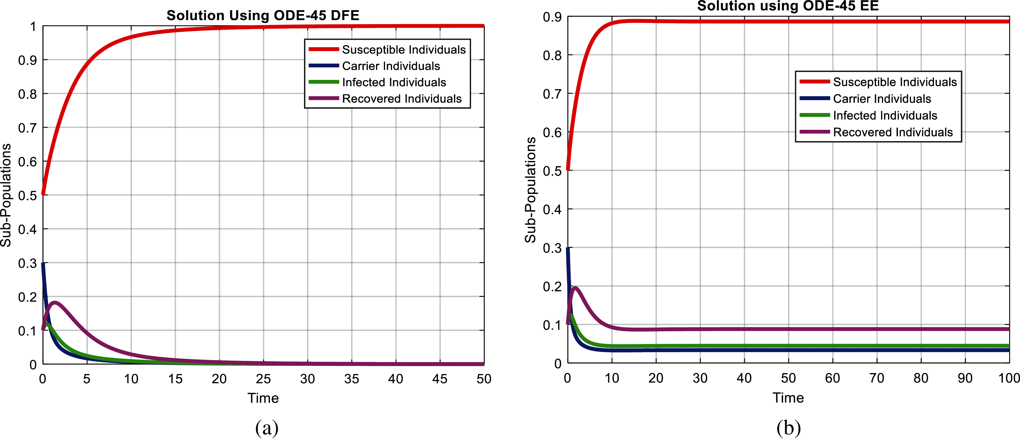
Figure 1: Combined graphical behaviors for DFE and EE at different subpopulations of the pneumonia disease (a) subpopulations for DFE at any time t (b) subpopulations for EE at any time t

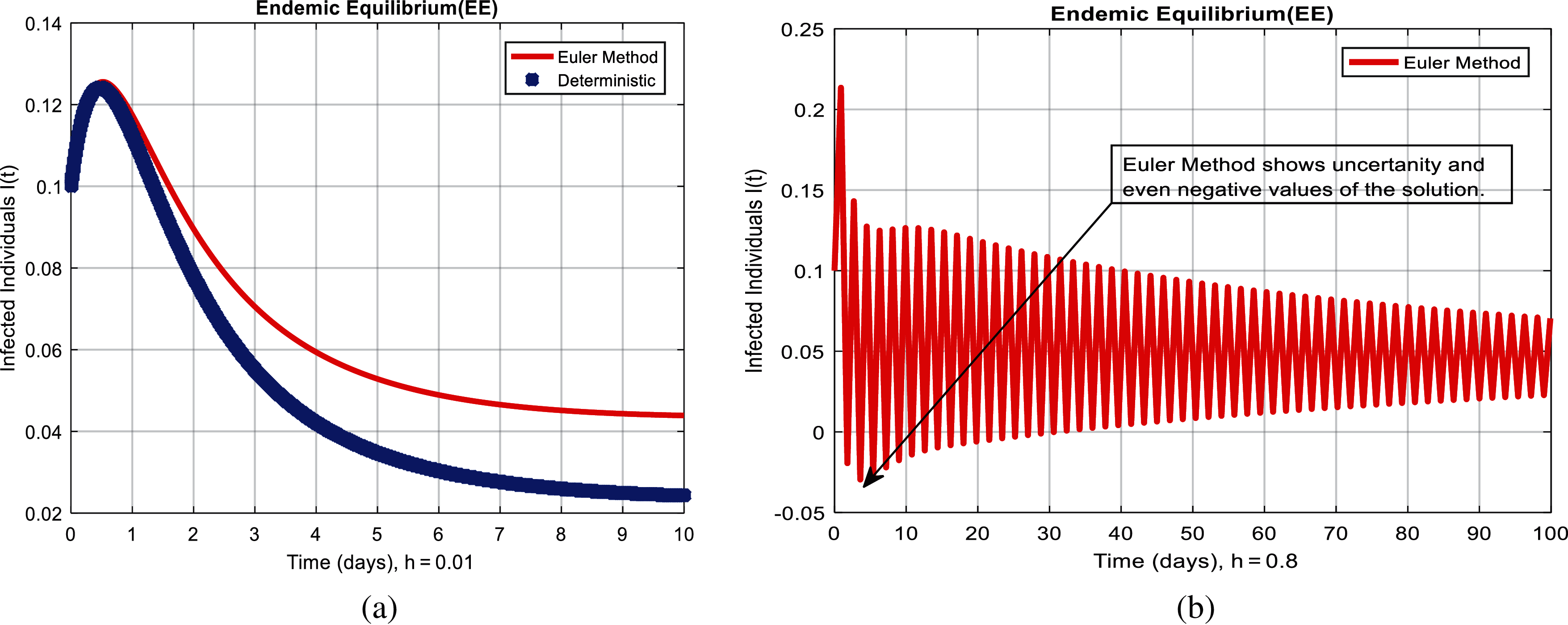
Figure 2: Euler method for the behavior of infected individuals at different time-step sizes (a) infected individuals at h=0.01 (b) infected individuals at h=0.8

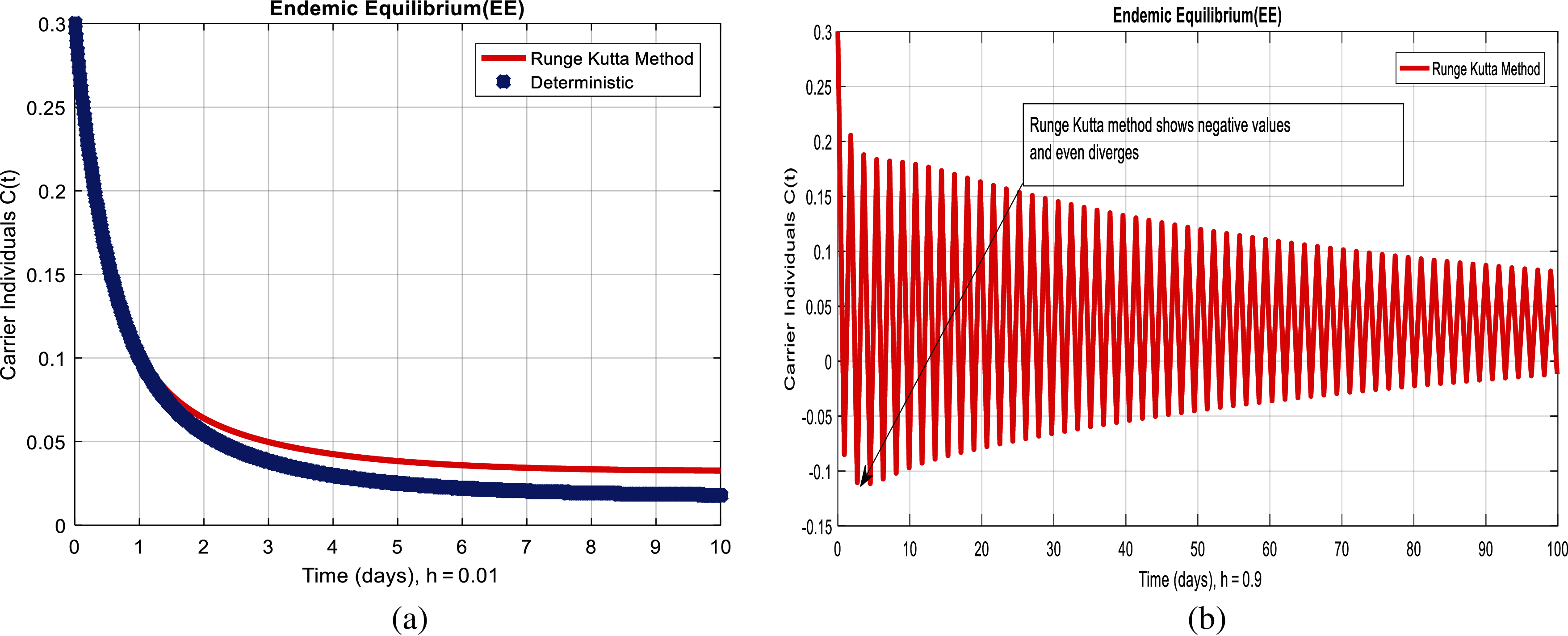
Figure 3: Runge Kutta method for the behavior of carrier individuals at different time-step sizes (a) carrier individuals at h=0.01 (b) carrier individuals at h=0.9

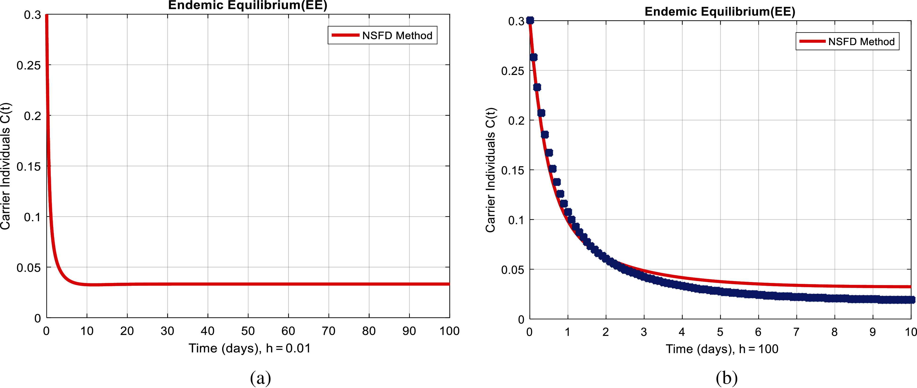
Figure 4: NSFD method for the behavior of carrier individuals at different time-step sizes (a) carrier individuals at h=0.01. (b) carrier individuals at h=100

5.6 Comparison Section

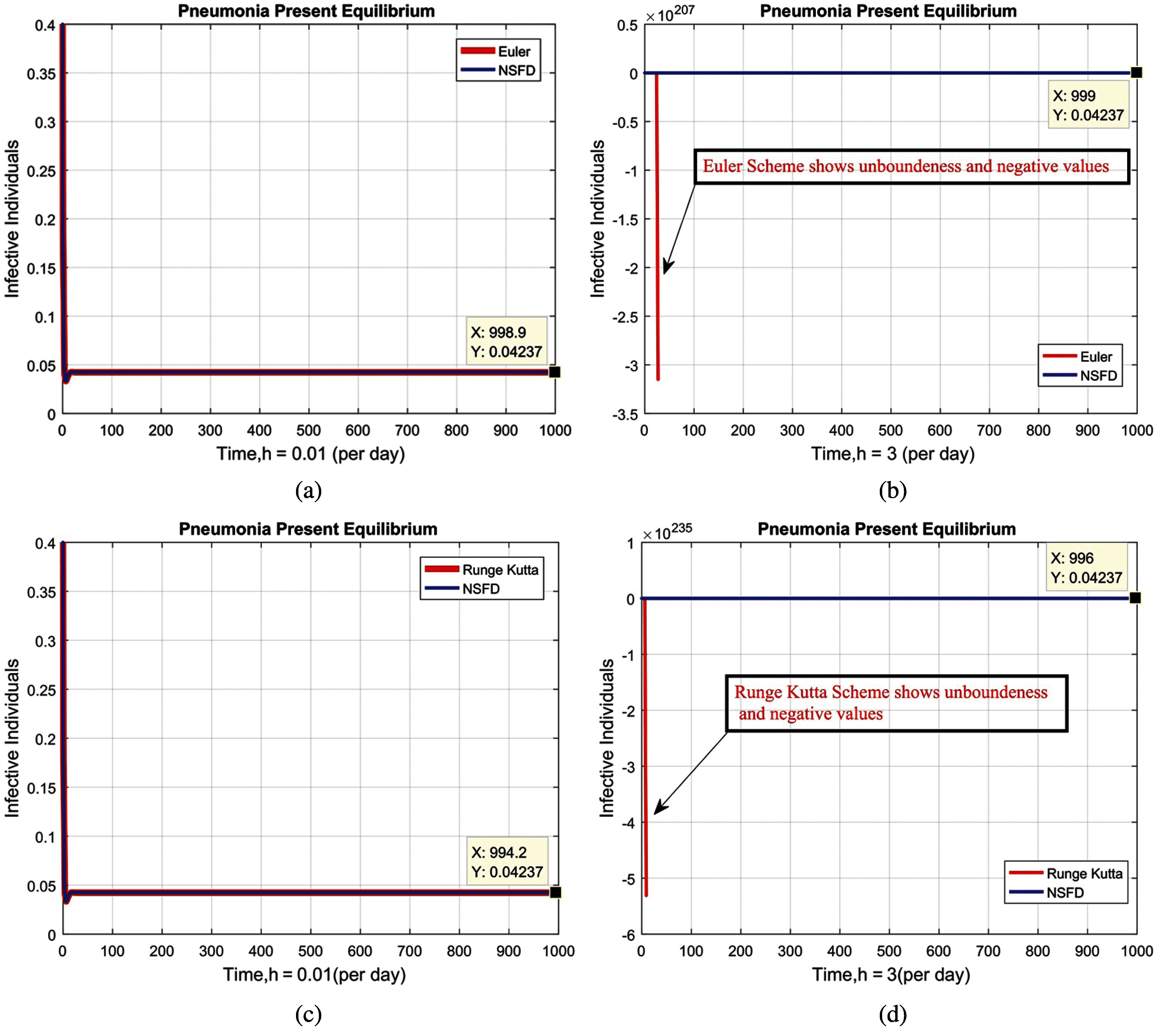
Figure 5: Combined graphical behaviors of NSFD with Euler and Runge Kutta methods at different time-step sizes (a) infective individuals for EE at h=0.01 (Euler and NSFD) (b) infective individuals for EE at h=3 (Euler and NSFD) (c) infective individuals for EE at h=0.01(Runge Kutta and NSFD) (d) infective individuals for EE at h=3(Runge Kutta and NSFD)

6  Results and Discussion

We present the solution to the system (1–4) via Matlab ordinary differential equations-45 at disease-free and endemic equilibria of the model in Figs. 1a and 1b. Also, the solutions of the system (5–8) via the Euler method at different time step sizes are in Figs. 2a and 2b. The solution of the system (9) via the Runge Kutta method at different time step sizes is in Figs. 3a and 3b. In the same, we plot the solutions of the system (10–13) via the NSFD method in Figs. 4a and 4b. In Figs. 5a–5d, the comparison section shows the investigation of computer methods such as Euler and Runge Kutta with NSFD approximations. Here, we observe that Euler and Runge Kutta show negativity and unboundedness and violate the dynamical properties of the model. However, our proposed numerical approximation is reliable, inexpensive, independent of the time step, and an efficient computational method.

7  Conclusion

We here investigated analyses of pneumonia infections via well-known computing techniques. Computer results of epidemic models are an authentic tool to cross-check the dynamical analysis of the model. For the sake of computational analysis, Euler, Runge Kutta, and the non-standard finite difference techniques (NSFD) are presented. Throughout the analysis, we observe that Euler and Runge Kutta are time-dependent techniques. Even when we increase the duration of the time step, these techniques violate such dynamic properties as positivity, boundedness, and dynamical consistency. However, NSFD is always convergent and independent of the size of the time step. These things could be observed from the comparison section. This idea could be extended to different types of disease modeling.

Acknowledgement: We thank LetPub (https://www.letpub.com) for its linguistic assistance during the preparation of this manuscript.

Funding Statement: The authors received no specific funding for this study.

Conflicts of Interest: The authors declare that they have no conflicts of interest to report regarding the present study.

References

 1.  E. Mochan, D. Swigon, G. Ermentrout, S. Luken and G. A. Clermont, “Mathematical model of intra-host pneumococcal pneumonia infection dynamics in murine strains,” Journal of Theoretical Biology, vol. 35, no. 3, pp. 44–54, 2014. [Google Scholar]

 2.  G. L. Drusano, W. Liu, S. Fikes, R. Cirz, N. Robbins et al., “Interaction of drug-and granulocyte-mediated killing of pseudomonas aeruginosa in a murine pneumonia model,” The Journal of Infectious Diseases, vol. 210, no. 8, pp. 1319–1324, 2014. [Google Scholar]

 3.  E. J. Ndelw, M. Kgosimore, F. S. Massawe and L. Namkinga, “Mathematical modelling and analysis of treatment and screening of pneumonia,” Mathematical Theory and Modeling, vol. 05, no. 10, pp. 21–39, 2015. [Google Scholar]

 4.  K. Kosasih, U. R. Abeyratne, V. Swarnkar and R. Triasih, “Wavelet augmented cough analysis for rapid childhood pneumonia diagnosis,” IEEE Transactions on Biomedical Engineering, vol. 62, no. 4, pp. 1185–1194, 2015. [Google Scholar]

 5.  A. C. G. Cesar, L. F. C. Nascimento, K. C. C. Mantovani and L. C. P. Vieira, “Fine particulate matter estimated by mathematical model and hospitalizations for pneumonia and asthma in children,” Revista Paulista de Pediatria, vol. 03, no. 4, pp. 18–23, 2016. [Google Scholar]

 6.  C. Marchello, A. P. Dale, T. N. Thai, D. S. Han and M. H. Ebell, “Prevalence of atypical pathogens in patients with cough and community-acquired pneumonia: A meta-analysis,” the Annals of Family Medicine, vol. 14, no. 6, pp. 552–566, 2016. [Google Scholar]

 7.  Y. H. Cheng, S. H. You, Y. J. Lin, S. C. Chen, W. Y. Chen et al., “Mathematical modeling of post co-infection with influenza a virus and streptococcus pneumoniae with implications for pneumonia and COPD-risk assessment,” International Journal of Chronic Obstructive Pulmonary Disease, vol. 12, no. 8, pp. 1973–1989, 2017. [Google Scholar]

 8.  K. Kosasih and U. Abeyratn, “Exhaustive mathematical analysis of simple clinical measurements for childhood pneumonia diagnosis,” World Journal of Pediatrics, vol. 13, no. 5, pp. 446–456, 2017. [Google Scholar]

 9.  G. T. Tilahun, O. D. Makinde and D. Malonza, “Modelling and optimal control of pneumonia disease with cost-effective strategies,” Journal of Biological Dynamics, vol. 11, no. 2, pp. 400–426, 2017. [Google Scholar]

10. M. Raj, M. Reddy, M. Mufeed and S. Karthika, “HMM based cough sound analysis for classifying asthma and pneumonia in pediatric population,” International Journal of Pure and Applied Mathematics, vol. 118, no. 18, pp. 609–616, 2018. [Google Scholar]

11. M. Kizito and J. Tumwiine, “A mathematical model of treatment and vaccination interventions of pneumococcal pneumonia infection dynamics,” Journal of Applied Mathematics, vol. 20, no. 18, pp. 01–16, 2018. [Google Scholar]

12. F. K. Mbabazi, J. Y. T. Mugisha and M. Kimathi, “Modeling the within-host co-infection of influenza a virus and pneumococcus,” Applied Mathematics and Computation, vol. 33, no. 9, pp. 488–506, 2018. [Google Scholar]

13. G. T. Tilahun, O. D. Makinde and D. Malonza, “Co-dynamics of pneumonia and typhoid fever diseases with cost effective optimal control analysis,” Journal of Applied Mathematics and Computation, vol. 31, no. 6, pp. 438–459, 2018. [Google Scholar]

14. G. T. A. Tilahun, “Optimal control analysis of pneumonia and meningitis confection,” Computational and Mathematical Methods in Medicine, vol. 20, no. 19, pp. 01–15, 2019. [Google Scholar]

15. M. Naveed, D. Baleanu, M. Rafiq, A. Raza, A. H. Soori et al., “Dynamical behavior and sensitivity analysis of a delayed coronavirus epidemic model,” Computers, Materials and Continua, vol. 65, no. 1, pp. 225–241, 2020. [Google Scholar]

16. K. Kosasih and U. Abeyratne, “Exhaustive mathematical analysis of simple clinical measurements for childhood pneumonia diagnosis,” World Journal of Pediatrics, vol. 13, no. 5, pp. 446–456, 2019. [Google Scholar]

17. G. T. Tilahun, “Modeling co-dynamics of pneumonia and meningitis diseases,” Advances in Difference Equations, vol. 20, no. 19, pp. 01–18, 2019. [Google Scholar]

18. F. K. Mbabazi, J. Y. Mugisha and M. Kimathi, “Hopf-bifurcation analysis of pneumococcal pneumonia with time delays,” Abstract and Applied Analysis, vol. 20, no. 19, pp. 01–36, 2019. [Google Scholar]

19. D. Otoo, P. Opoku, S. Charles and A. P. Kingsley, “Deterministic epidemic model for pneumonia dynamics with vaccination and temporal immunity,” Infectious Disease Modelling, vol. 05, no. 1, pp. 42–60, 2020. [Google Scholar]

20. O. C. Zephaniah, U. I. R. Nwaugonma, I. S. Chioma and O. Adrew, “A mathematical model and analysis of an SVEIR model for streptococcus pneumonia with saturated incidence force of infection,” Mathematical Modeling and Applications, vol. 05, no. 1, pp. 01–16, 2020. [Google Scholar]

21. A. Raza, M. S. Arif and M. Rafiq, “A reliable numerical analysis for stochastic gonorrhea epidemic model with treatment effect,” International Journal of Biomathematics, vol. 12, no. 5, pp. 445–465, 2019. [Google Scholar]

22. S. M. Jung, R. Kinoshita, R. N. Thompson, N. M. Linton, Y. Yang et al., “Epidemiological identification of a novel pathogen in real time: Analysis of the atypical pneumonia outbreak,” Journal of Clinical Medicine, vol. 09, no. 3, pp. 01–18, 2020. [Google Scholar]

23. P. Saha, D. Mukherjee, P. K. Singh, A. Ahmadian, M. Ferrara et al., “Graphcovidnet: A graph neural network-based model for detecting COVID-19 from CT scans and X-rays of chest,” Scientific Reports, vol. 11, no. 1, pp. 01–20, 2021. [Google Scholar]

24. V. Gupta, N. Jain, P. Katariya, A. Kumar, S., Mohan et al., “An emotion care model using multimodal textual analysis on COVID-19,” Chaos, Solitons & Fractals, vol. 144, no. 1, pp. 01–18, 2021. [Google Scholar]

25. N. Jain, S. Jhunthra, H. Garg, V. Gupta, S. Mohan et al., “Prediction modelling of COVID using machine learning methods from B-cell dataset,” Results in Physics, vol. 21, no. 1, pp. 01–19, 2021. [Google Scholar]

26. N. Jain, A. Ghosh, S. P. Mondal, M. Y. Bajuri, A. Ahmadian et al., “Identification of dominant risk factor involved in spread of COVID-19 using hesitant fuzzy MCDM methodology,” Results in Physics, vol. 21, no. 2, pp. 01–15, 2021. [Google Scholar]

27. A. Raza, A. Ahmadian, M. Rafiq, S. Salashour, M. Naveed et al., “Modeling the effect of delay strategy on transmission dynamics of HIV/AIDS disease,” Advances in Difference Equations, vol. 663, no. 1, pp. 01–19, 2020. [Google Scholar]

28. N. Ahmed, A. Raza, M. Rafiq, A. Ahmadian, N. Batool et al., “Numerical and bifurcation analysis of SIQR model,” Chaos, Solitons and Fractals, vol. 150, no. 1, pp. 01–15, 2021. [Google Scholar]

29. J. E. M. Diaz, A. Raza, N. Ahmed and M. Rafiq, “Analysis of a nonstandard computer method to simulate a nonlinear stochastic epidemiological model of coronavirus-like diseases,” Computer Methods and Programs in Biomedicine, vol. 204, no. 1, pp. 01–10, 2021. [Google Scholar]

30. A. Akgul, M. S. Iqbal, U. Fatima, N. Ahmed, Z. Iqbal et al., “Optimal existence of fractional order computer virus epidemic model and numerical simulations,” Mathematical Methods in the Applied Sciences, vol. 7437, no. 1, pp. 01–13, 2021. [Google Scholar]

31. U. Fatima, D. Baleanu, N. Ahmed, S. Azam, A. Raza et al., “Numerical study of computer virus reaction diffusion epidemic model,” Computers, Materials and Continua, vol. 66, no. 3, pp. 3183–3194, 2021. [Google Scholar]

32. A. Raza, A. Ahmadian, M. Rafiq, S. Salahshour and I. R. Laganà, “An analysis of a nonlinear susceptible-exposed-infected-quarantine-recovered pandemic model of a novel coronavirus with delay effect,” Results in Physics, vol. 21, no. 1, pp. 01–07, 2021. [Google Scholar]

33. W. Shatanawi, A. Raza, M. S. Arif, M. Rafiq, M. Bibi et al., “Essential features preserving dynamics of stochastic dengue model,” Computer Modeling in Engineering and Sciences, vol. 126, no. 1, pp. 201–215, 2021. [Google Scholar]

34. A. Raza, M. S. Arif, M. Rafiq, M. Bibi, M. Naveed et al., “Numerical treatment for stochastic computer virus model,” Computer Modeling in Engineering and Sciences, vol. 120, no. 2, pp. 445–465, 2019. [Google Scholar]

35. M. S. Arif, A. Raza, K. Abodayeh, M. Rafiq and A. Nazeer, “A numerical efficient technique for the solution of susceptible infected recovered epidemic model,” Computer Modeling in Engineering and Sciences, vol. 124, no. 2, pp. 477–491, 2020. [Google Scholar]

36. W. Shatanawi, A. Raza, M. S. Arif, M. Rafiq, M. Bibi et al., “Essential features preserving dynamics of stochastic dengue model,” Computer Modeling in Engineering and Sciences, vol. 126, no. 1, pp. 201–215, 2021. [Google Scholar]

37. M. A. Noor, A. Raza, M. S. Arif, M. Rafiq, K. S. Nisar et al., “Non-standard computational analysis of the stochastic COVID-19 pandemic model: An application of computational biology,” Alexandria Engineering Journal, vol. 61, no. 1, pp. 619–630, 2021. [Google Scholar]

38. K. Abodayeh, A. Raza, M. S. Arif, M. Rafiq, M. Bibi et al., “Numerical analysis of stochastic vector borne plant disease model,” Computers, Materials and Continua, vol. 63, no. 1, pp. 65–83, 2020. [Google Scholar]

39. K. Abodayeh, A. Raza, M. S. Arif, M. Rafiq, M. Bibi et al., “Stochastic numerical analysis for impact of heavy alcohol consumption on transmission dynamics of gonorrhoea epemic,” Computers, Materials and Continua, vol. 62, no. 3, pp. 1125–1142, 2020. [Google Scholar]

40. H. Jansen and E. H. Twizell, “An unconditionally convergent discretization of the SEIR model,” Mathematics and Computer Simulation, vol. 58, no. 1, pp. 147–158, 2002. [Google Scholar]

This work is licensed under a Creative Commons Attribution 4.0 International License, which permits unrestricted use, distribution, and reproduction in any medium, provided the original work is properly cited.