Energy Efficiency Trade-off with Spectral Efficiency in MIMO Systems

Rao Asif; Mustafa Shakir; Jamel Nebhen; Ateeq Rehman; Muhammad Shafiq; Jin-Ghoo Choi

doi:10.32604/cmc.2022.020777

Rao Muhammad Asif1, Mustafa Shakir1, Jamel Nebhen2, Ateeq Ur Rehman3, Muhammad Shafiq4,* and Jin-Ghoo Choi4

1Department of Electrical Engineering, Superior University, Lahore, 54000, Pakistan
2College of Computer Engineering and Sciences, Prince Sattam Bin Abdulaziz University, Alkharj, 11942, Saudi Arabia
3Department of Electrical Engineering, Government College University, Lahore, 54000, Pakistan
4Department of Information and Communication Engineering, Yeungnam University, Gyeongsan, 38541, Korea
*Corresponding Author: Muhammad Shafiq. Email: shafiq@ynu.ac.kr
Received: 06 June 2021; Accepted: 07 August 2021

Abstract: 5G technology can greatly improve spectral efficiency (SE) and throughput of wireless communications. In this regard, multiple input multiple output (MIMO) technology has become the most influential technology using huge antennas and user equipment (UE). However, the use of MIMO in 5G wireless technology will increase circuit power consumption and reduce energy efficiency (EE). In this regard, this article proposes an optimal solution for weighing SE and throughput tradeoff with energy efficiency. The research work is based on the Wyner model of uplink (UL) and downlink (DL) transmission under the multi-cell model scenario. The SE-EE trade-off is carried out by optimizing the choice of antenna and UEs, while the approximation method based on the logarithmic function is used for optimization. In this paper, we analyzed the combination of UL and DL power consumption models and precoding schemes for all actual circuit power consumption models to optimize the trade-off between EE and throughput. The simulation results show that the SE-EE trade-off has been significantly improved by developing UL and DL transmission models with the approximation method based on logarithmic functions. It is also recognized that the throughput-EE trade-off can be improved by knowing the total actual power consumed by the entire network.

Keywords: Energy efficiency; spectral efficiency; throughput; massive MIMO; downlink; uplink; base stations; power consumption

With the current revolution of 5G wireless cellular technology and its achievements in large-scale multiple input multiple output (MIMO) systems, wireless networks have been optimized by 10 times in terms of efficiency, spectral efficiency (SE) and throughput. The existing standards for 3G and 4G mobile networks cannot meet the challenging pace of data rates, and the number of antennas is huge, because they can only allow up to 8 antenna ports [1]. Massive MIMO has the ability to handle applications with high data rates base stations (BS) with a large number of antennas and efficient services for users. The development and progress of this emerging technology show that massive MIMO has become a gold mine of research progress in the field of wireless communications [2]. In addition, although a large number of antennas are managed at a BS with a much more complex system, it provides higher efficiency, SE and throughput [3]. On the other hand, in the past 30 years, the average data rate of wireless data transmission has doubled every 18 months [4]. The 5G mobile network standard is under consideration. However, rapid development and urgent needs encourage the use of the 33–46 GHz frequency band during the test phase, where 5G practices the unfinished standard at the 28 GHz frequency [5].

The old wireless network system faces complexity, such as low reliability, poor connection, low efficiency, low energy efficiency, low spectrum efficiency, and low throughput. The number of mobile-connected smart devices and smart phone users on existing cellular networks has grown exponentially. Considering the above facts and Martin Cooper's law requirements (data and voice doubled every 2.5 years), there is an urgent need for high-quality services and optimized wireless networks to increase capacity and connectivity to meet future needs [6]. In this regard, the energy efficiency (EE) of massive MIMO systems has become an urgent consideration in 5G because it involves a large number of antennas and increased circuit power consumption (PC). Massive MIMO systems can handle all technical issues, optimizing EE by processing more antennas and reasonable circuit power consumption [7].

The massive MIMO model has great potential in 5G [8]. It has thousands of antennas and can provide higher specytum effeciency and energy effeciency. However, each antenna is assigned a dedicated frequency, including digital-to-analog converters and analog-to-digital converters, and noise amplifiers. For this reason, a large number of active antennas have been adopted, consuming more power. Therefore, the hardware cost in BS has increased. By providing more antennas for many users on the same radio channel frequency, the spectrum efficiency can be significantly improved. However, power consumption requirements reduce the advantages of energy efficiency. It has been experienced in previous systems that minimizing the low resolution triggered by power consumption is disadvantageous.

The optimization method of spectrum efficiency and energy efficiency should make it possible to connect the best number of antennas with the least power consumption. massive MIMO has been recently proposed, which is a potential technology that can enhance network throughput and energy efficiency [9,10]. Throughput is affected by the efficiency of spatial multiplexing based on antenna channel effects [11]. Due to concerns about the hardware cost of power consumptions and a large number of antennas, the use of more efficient hardware and low-cost circuits has reduced the throughput of the network. The energy efficiency of the network depends on less power consumptions. Following are the authors’ contributions to the trade-off between energy efficiency and throughput:

• We considered a multi-cell scenario, in which uplink (UL) and downlink (DL) transmissions are calculated based on the Wyner model and computed the optimized relations for selecting numbers of UEs and multiple antennas.

• We optimized the parameters for selecting optimal antennas and users through an approximation method based on a logarithmic function and verified the SE-EE optimization relationship.

• We formed expressions in the massive MIMO network of UL and DL models and calculated different combinations and precoding schemes simultaneously.

• We also formulated the optimal trade-off between throughput-EE using combining and precoding schemes by considering total circuit power consumption.

The rest of this paper is organized as follows. Section 2 summarizes the related work. Section 3 introduces the system model proposed for UL and DL in Wyner model. Section 4 investigates the EE-SE trade-off and calculates the optimal relationship for selecting multiple antennas and UEs. Section 5 calculates the complete actual power and studies the combination of UL and DL networks and precoding schemes. Section 6 discusses the results and validates the model. The last section draws our conclusions.

The power consumption and throughput of the user equipment decrease in a large-scale MIMO system. So, the trade-off between SE and EE and network throughput becomes crucial. We can find a power consumption model in [12], in which a closed-form approximation model for the uplink network is proposed to obtain ideal method for the trade-off between EE and SE. In [13], authors consider an evaluation criterion for the trade-off between EE and SE. The Rayleigh fading (RF) channels have been evaluated using a more general closed-form approximation method. This model compared with a single-input single-output (SISO) network and shows that when the PC model is considered, the MIMO system is an EE enhancer and reduces the number of antennas on the transmitter side.

In [14], the uplink and downlink system models of the distributed MIMO network are composed of various PC models to drive the expression of trade-offs, and the strength of the digital antenna is optimized by considering the PC model. In [15–17], Maximum Ratio combination scheme-based approximation is used for the trade-off between EE and SE. This model shows that adding antennas can increase efficiency but reduce SE, the best value of SE that can maximize EE.

The model proposed in [18] has considered the PC model of the transceiver PC and the radiating PC, and at the same time uses a tight expression form to achieve the best EE-SE trade-off. In [19], the method based on the Pareto optimal set uses the proposed multi-objective optimization method to calculate the EE-SE compromise method. The method takes into account the number of antennas available at the PC and BS, and the Cobb-Douglas production model calculates a trade-off matrix to convert the optimization function into a single objective function. As a result, an optimized PC for the largest available antenna in the network is realized that optimize the trade-off through various priorities.

In [20–22], authors consider the channel state information of the transmitter to derive the expression of the signal-to-noise ratio based on the number of PCs and antennas to optimize the trade-off. In [23], the author proposed two algorithms for complex optimization methods to obtain optimization in EE-SE trade-off. The original algorithm is practiced through the improved Big Grey Wolf optimization algorithm. The second algorithm is the improved Lion algorithm, which is formed to increase the convergence speed and help make a better trade-off between SE and EE. In [24], a user-centric (UC) access point selection method has been proposed to improve the performance of the MIMO system. In [25], the effect of antenna channel on MIMO throughput calculated that the spatial multiplexing efficiency would be reduced due to power imbalance. In [9], the author developed a model to maximize throughput and EE. In [19], we can also find another model that contains 400 antennas and multiple transmitters for throughput analysis. This model provides a detailed background for studying the EE and throughput of wireless networks. In [25], a further throughput analysis is proposed by considering some approximations and assumptions. However, the proliferation UEs and limitations on power consumption have made the trade-off between SE and EE and network throughput open. However, the surge of UEs and the limitation of power consumption make the optimization of throughput, SE and EE trade-offs a real challenge. We also need to consider the trade-offs of EE, SE, and throughput in the same system to give full play to the advantages of 5G technology.

The system model describes UL and DL transmission models in a multi-cell scenario. We assume the Wyner model for UL and DL transmission because it is simple and analytical tractable. As shown in Fig. 1, the two-cell network composed of cell j and cell l describes the system model of interface signals and desired signals during inter-cell and intra-cell interferences. Therein, we also consider signal-to-noise-ratio (SNR) as weight parameter. 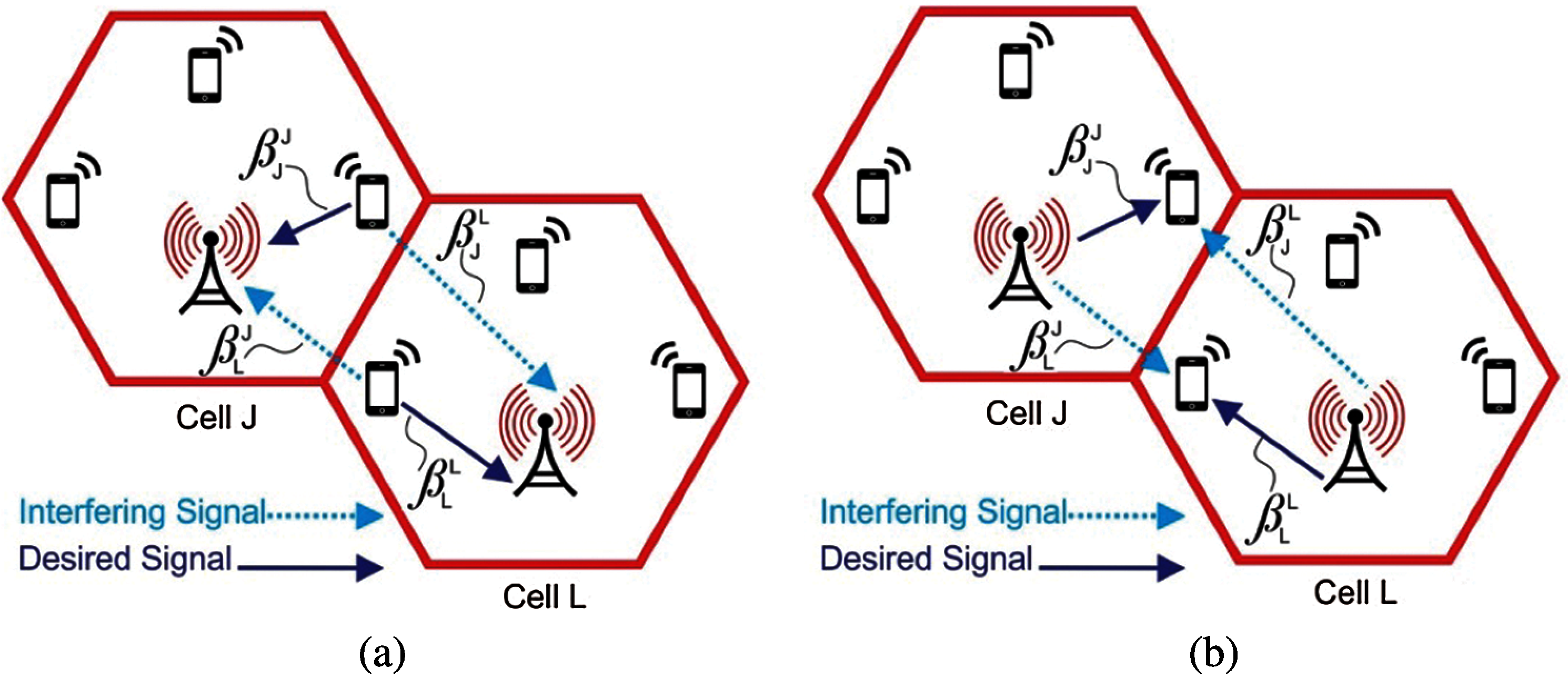The notations βll, βll, βlj, βjj, and βjl and each UE in cell l preserves the same average channel gain βll from BS to be served [24]. The average channel gain βlj is also similar for that of BS of the cell j when each UE in cell j has same average gain as βjl and βjj. The Wyner model specifies that intra-cell gain and inter-cell gain are equal as assumed i.e., βll=βjj and βlj=βjl. The ratio of inert-cell and intra-cell channels gain are formed as follows,

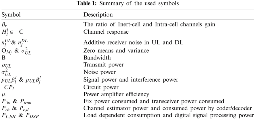
Figure 1: System model for the desired and interfering signals in Cell l and Cell j: (a) UL Transmission; (b) DL transmission

The ratio of average gain used in the modeling βr varies in [0–1] where βr close to 0 indicates that inter-cell interference is small, and βr a value close to 1 means it is strong. The channel response symbols used in this paper are Hll∈C and Hjl ∈C and the relation with channel gain is written as,

Based on the above facts, the following is the model of UL and DL transmission signals. Before we proceed, we have described a summary of the used symbols in Tab. 1.

For the enhancement of SE, we illustrate the UL transmission based on the Wyner model in Fig. 1a. We assume k active UEs in each cell under UL network. The channel response of kth desired UE in a cell l and BS is given by Hlkl€ CM up to k = 1 to k=K and the channel response is as follows,

where SjkUL is the kth UE signal in cell l, the the receiver noise denoted by nlUL∼CN(OMj,σUL2{\rm I}Ml). The terms OMj and σUL2 are zero means and variance respectively. ρUL > 0 is used for the uplink SNR. Let BS of cell l receives a signal transmitted by the desired UEs as K, and UL signal ylkULϵ CM is given by,

VlkULylUL=ρUL VlkULHlklsliUL+ρUL ∑i=1i≠kKl⁡VlkULHlnlslnUL+ρUL ∑n=1Kn⁡VlkULHlilsjnUL+nlUL (4)

where ρUL VlkULHlklsliUL considered as the desired signal, ρUL ∑i=1i≠kKl⁡VlkULHlnlslnUL term formed as intra-cell interference, ρUL ∑n=1Kn⁡VlkULHlilsjnUL given as intercell interference, and nlUL is noise.

ρUL is used for transmitting power and σUL2 is noise power. Consider Eq. (1) and (6) for βr≠1 then SE can be formulated as follows,

where pULβll , pULβjl, and σUL2 are signal power, interference power, and noise power respectively.

For the enhancement of SE, we illustrate here the DL transmission based on the Wyner model in Fig. 1a. We discussed the average channel gain in the previous section. In the DL model, the Kth active UEs of each cell receives a signal send by serving BS using linear precoding schemes. Same as UL, the DL channel response of Kth active UEs of each cell receives a signal sent by serving BS is (Hlkl)H and received DL signal in cell l is modeled as,

yjdl=ρDLHlkl)HwlkrlkSlk+ρDL ∑i=1i≠kKl⁡(Hlkj)HWlirjiSli+ρDL ∑j=1j≠lL⁡∑i=1Kl⁡(HlkDL)HWlirlisji+nlDL (9)

where ρDLHlkl)Hwlkrlkslk is desired signal, with intra-cell interference, intercell interference, and noise signals respectively. Moreover, wlkrlkand slk are precoding vector and DL transmitted signal. As per Wyner model as Eq. (1), the βr relation with SE becomes,

SEl=∑k=1k⁡Log2(1+M∑i=1i ≠kk⁡G(φlil)+βr∑i=1k⁡G(φjij)+1SNRl) (10)

SEl=∑k=1K⁡E{Log2(1+ρDL |Hll|2ρDL∑k=1i≠kk⁡|HlklHlil|2|Hlil|2+ρDL∑i=1k⁡|HjklSjkUL|2|Hll|2+σDL2)}(11)

As discussed in the literature, SE will increase as more BS antennas and multiple UEs are installed in the cell, and this increase in SE will lead to an increase in PC. This phenomenon will reduce the overall EE, so a mechanism that can jointly improve SE and EE is needed. This section considers the Wyner model of the two-unit scheme shown in Fig. 1 to analyze the EE-SE trade-off. The selection of multiple antennas and UEs for optimizing the EE-SE trade-off is discussed in the following.

We defined an assumption of active UE in cell l and having no interfering signal. The SE in cell l is given as the first step in antenna selection in [26] as follows,

where ρUL is a transmit power, σUL2 is a noise power. To select numbers of the antenna (M) for the optimizing of EE, the circuit power (CP) is also evaluated as it increases when multiple antennas have selected. In this case, the cell l is chosen to have circuit power CPl then EE relation with M becomes with logarithm function-based approximation:

where ETP is effective to transmit power, and μ has a range in [0<μ≤1] for the power amplifier efficiency with bandwidth B. Hence,

The total power consumption has also M times power consumption of circuit components (PCC) power. Hence, Eq. (16) becomes,

We take M number of antennas, PCC as circuit consumption, CP as circuit power into account prior to [26] where M effects only one power consumption model and we modified based on the requirement as,

where log2(M CPl+MPCC) is SE. The final expression of selection for multiple antennas is given by,

As the number of UEs increases (such as the number of antennas), the SE increases with the increase in power consumption, resulting in a decrease in EE. As shown in Fig. 1, the Wyner model with K antenna in both cells having relative channel gain as Eq. (1), the SE of cell l is written as,

The tradeoff relation of EE-SE is formed in Eq. (22) prior to [28] and we computed,

where the power consumption of M times BS (MPCC), CPl, and K time UEs are considered. The change of EE concerning change in SE can show the tradeoff scenario. In this regard, the derivate of EE concerning SE is taken by logarithm function-based approximation as follows,

K(M−K(2SEl−1)−Kβr+M−K)−1ν0+CPl+MPCC+KPUE=K SEl(1−(2SEl−1M−K)Kβr−1+K)−2v0loge(2)M−K2SEl (23)

We put Eq. (23) into Eq. (22). Hence, the trade-off between EE and SE is optimized as,

In this section, we consider circuit power consumption model and the UL and DL model to optimize the trade-off between SE and throughput. In this model, the transmit power, circuit power consumed by hardware at the BS side, coding/decoding power, and digital signal processing power are as considered to evaluate the trade-off between EE and throughput. In this regard, the expression formed for the BS l in massive MIMO network [28] is given by,

where the CP model considers the fixed power (Pfix) consumed by transceiver (Ptran), channel estimator power (Pch) consumed power by coder/decoder (Pc,d), load-dependent consumption (PL,bH), and digital signal processing power (PDSP ). For the overall power consumed by BS l for the UL and DL, we simply derive the expression as follows,

where PSig is an overall power consumed in transmission and receiving of signal and PR,T, PComUL, and PPreDL are the transmitter/receiver power, combining vectors, and precoding vectors consumed power, respectively. PComUL and PPreDL both are computed for combining and precoding vector as follows,

The illustration of combining schemes as multicell MMSE, single-cell MMSE, RZF, ZF, and MR with their power consumption for the UL signal is derived in Tab. 2. For DL signals, the precoding vector in [29] uses the same vector. Our power consumption calculation model is written in Tab. 3. The power consumed by the transmission of the UL and DL signals through the pilot sequence can be written as,

TTPl=τpilτcoh∑k=1kl⁡1uUElpl+τULτcoh∑k=1kl⁡1uUElρUL+τDLτcoh∑k=1kl⁡1uUElρDL (29)

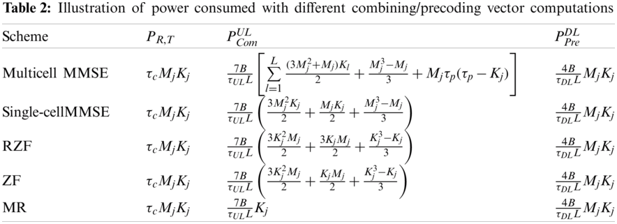
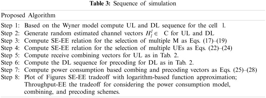
where total transmit power consist of the total transmit power of the pilot signal τpilτcoh∑k=1kl⁡1uUElpl, total transmit power of UL signal τULτcoh∑k=1kl⁡1uUElρUL, and that of DL signal τDLτcoh∑k=1kl⁡1uUElρDL. The simulation parameters and results are discussed in the next section.

We analyze the SE, EE, and throughput expressions of UL and DL using the simulation results. The model is simulated in MATLAB, and the simulation sequence is shown in Tab. 3. We select M antennas, and K UEs considering the throughput calculation of M-MMSE, S-MMSE, RZF, ZF, MR combining and precoding schemes. In the first step, the two-cell network composed of cell j and cell l assumes the Wyner model of interface signals and desired signals during inter-cell and intra-cell interferences. The ratio of inert-cell and intra-cell channel gain is formed in Eq. (1) and UL and DL sequences for the cell are computed in Section 3. The second step generates random estimated channel vectors of desired UE in a cell, and BS is given by Hlkl€ CM up to k = 1 to k=K as given in Eq. (3) for UL transmission. Same as UL, the DL channel response (Hlkl)H is generated by active and BS while the SE, SNR, and channels gain are also taken into account as computed in sections 3.1 and 3.2. In third step, SE-EE relation is computed for the selection of M number of antennas by considering PCC, and CP as computed in Eqs. (17)–(19). Fourth step computes the SE-EE relation for the selection of multiple UEs as formulated in Eqs. (22)–(24) where MPCC, CPl, and K time UEs are considered. The change of EE concerning change in SE computes tradeoff scenario and the derivate of EE concerning SE is taken by logarithm function-based approximation. Fifth step computes the combining schemes as multicell MMSE, single-cell MMSE, RZF, ZF, and MR with their power consumption for the UL signal is derived in Tab. 2. In next step, DL signal for computing the precoding vector uses the same vector as used in UL. The power consumed by the transmission of the UL and DL signals through the pilot sequence is computed in Eq. (29). Step.7 computes the power consumption-based combing and precoding vectors as given in Eqs. (25)–(28) by considering the Pfix consumed by transceiver (Ptran), Pch consumed power by coder/decoder (Pc,d), load-dependent consumption (PL,bH), and digital signal processing power (PDSP ). Last step of simulation sequence generates the plots for SE-EE tradeoff with logarithm-based function approximation. The optimal tradeoff of EE with SE and throughput is discussed in detail as follows.

As discussed that CPl increases with M times in the selection of multiple antennas as Eq. (16). Fig. 2a illustrates the SE-EE tradeoff. The x-axis represents the SE in Bit/s/Hz and the y-axis represents the EE in bit/joule. The results of Fig. 2a are elaborated in Tab. 5 where CPl=0,5,10,15 Watts are considered, numbers of antennas are 10 with a bandwidth of 200 KHz, σ2β00= −3dBm, and μ=0.5. As shown in Fig. 2a and concluded in Tab. 5, for the optimal tradeoff the SE increases from 0 to 10 [Bit /s/Hz] when CPl wattage increased up to 15 watts but decreases the EE from 2×107 to 2.5×105 as [21] expresses this fact. The optimal points for the tradeoff of SE-EE are shown in Fig. 2a that are improved as compared to [23] where our model has less effect of the decline in EE at given parameters.

As computed in Eqs. (18) and (19), the CPl +ETP are fixed as 15 w and 2 watt with Multiple M for optimizing the tradeoff of SE-EE illustrated in Fig. 2b. The x-axis represents the SE in Bit /s/Hz and the y-axis represents the EE in bit/joule. In Tabs. 4 and 5, we inscribed the simulation parameters used for the simulation results shown in Fig. 2, where M=5, 20, 100, 1000 are considered with a bandwidth of 200 KHz, σ2β00= −3dBm, and μ=0.5. In Fig. 2, we can see that the optimal tradeoff of SE increases from 2 to 10.5 [Bit /s/Hz] with several multiple antennas. However, the CPl+ETP wattages are fixed while it decreases the EE from 2×105 to 1.8×104. We see that the optimal points for the tradeoff of SE-EE are improved compared to that of [23]. As computed in Eqs. (23) and (24), different M/K ratio is taken into account for optimizing the tradeoff of SE-EE. In Fig. 3, the x-axis represents the SE in Bit /s/Hz and the y-axis represents the EE in bit/joule. The simulation parameters regarding the simulation results in Fig. 3 are shown in Tab. 6, where M/k=2, 4, 8, 16 are considered with the same bandwidth, σ2β00, and μ used in multiple antenna selections. We see the optimal tradeoff in Fig. 3, where the SE increases from 14 to 48 [Bit /s/Hz] as it increases with several multiple antennas while the notable parameter is that there is not much decrement in EE as it only decreases 3×105 to 4×105. The optimal points for the tradeoff of SE-EE are shown in Fig. 3a that are improved as compared to that of [22].

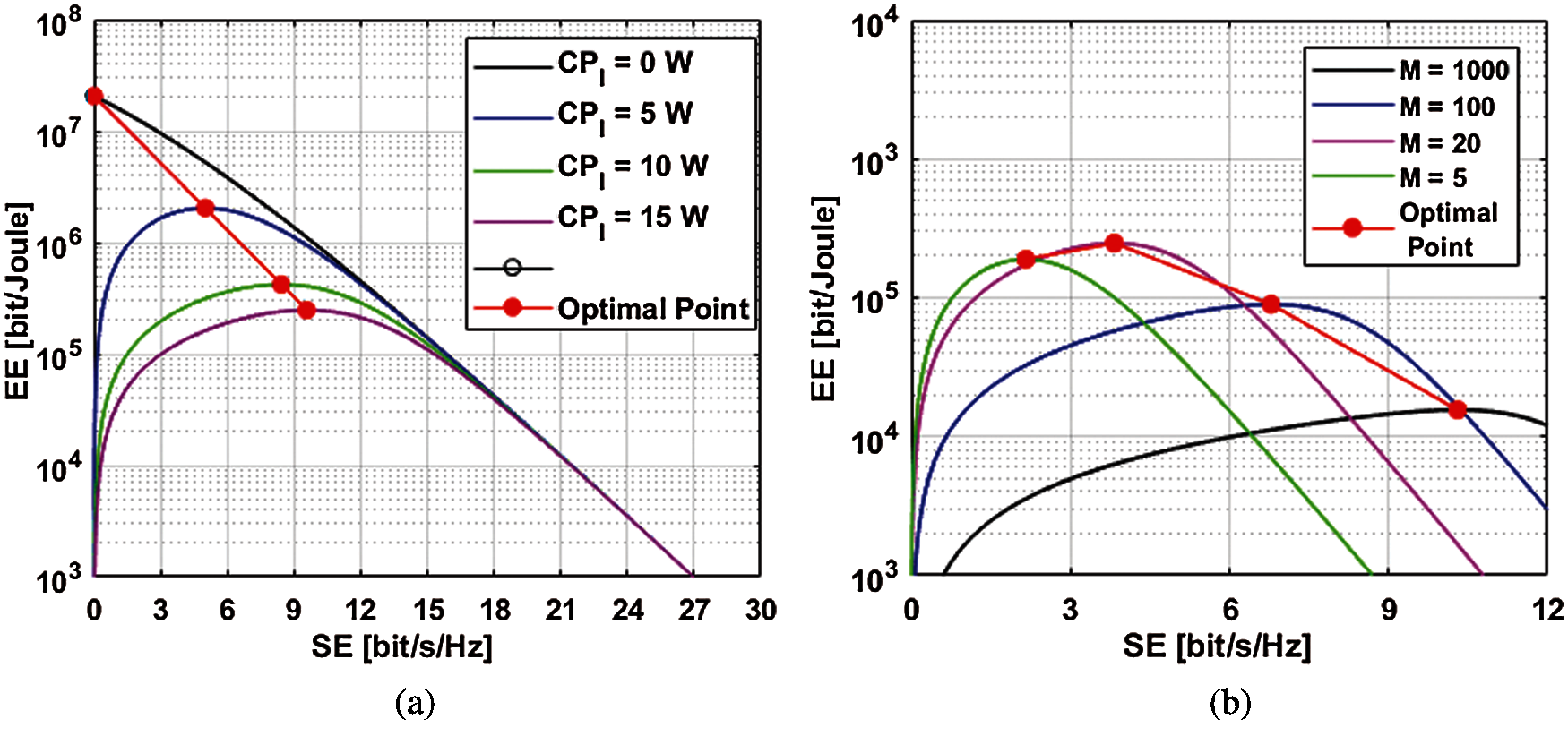
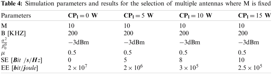
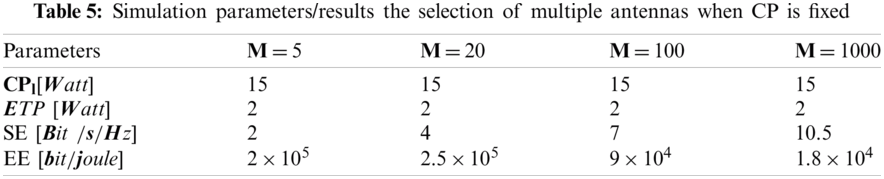
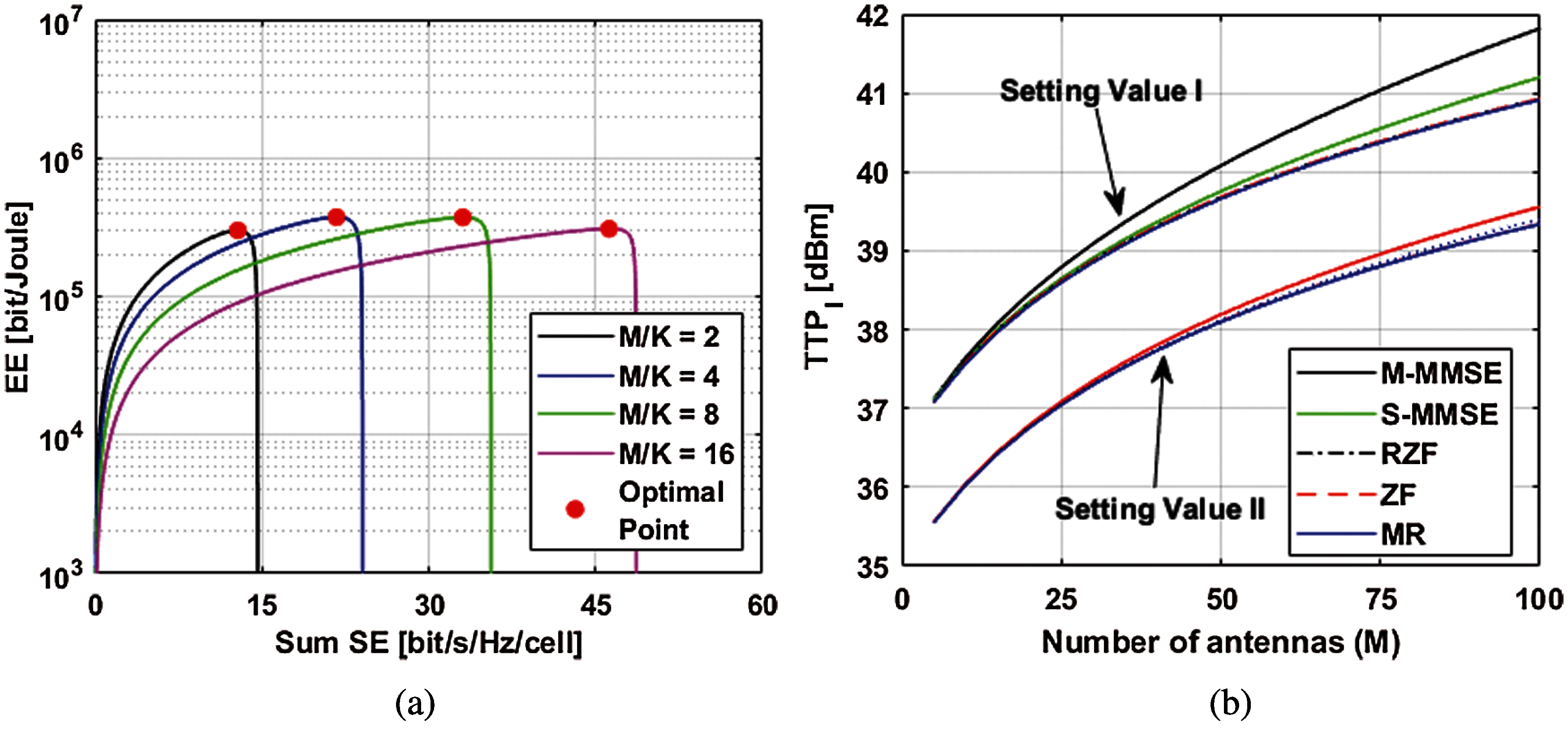
Figure 2: Throughput-EE tradeoff: (a) for different CPl in the case of Me antenna selections (b) for different M in case of multiple antenna selections

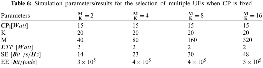
Figure 3: EE-SE tradeoff: (a) when different M/K are considered in case of multiple UEs selection (b) Results of multiple CP models of two setting values with different combining/precoding schemes

The trade-off between EE and throughput is slightly different because it caters to all power consumption models of UL and DL with different combining and precoding schemes schemes, as shown in Tab. 3. In order to find the total power consumption of all the models calculated in this section, multiple antennas are considered. Figs. 3b and 4b show the results.

The x-axis represents the varying numbers of of antennas, and the y-axis represents TTP in dBm. Various power consumption parameters are given in the Tab. 3. The best trade-off requires the total transmit power of all combing and precoding vectors, such as 41.8, 41.2, 40.9, 40.9 and 40.9 dBm of M-MMSE, S-MMSE, RZF, ZF and MR. The setting value-I is shown in Fig. 3b. Therein, we observe that after setting the power consumption value to half, the dBm of M of ZM, RZF, M-MMSE, S-MMSE and MR are reduced to 39.5, 39.45, 39.40, 39.40 and 39.40 dBm, respectively. Set value-II shown the Tab. 7.

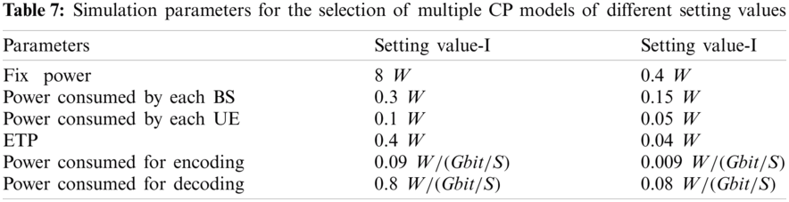
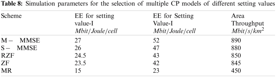
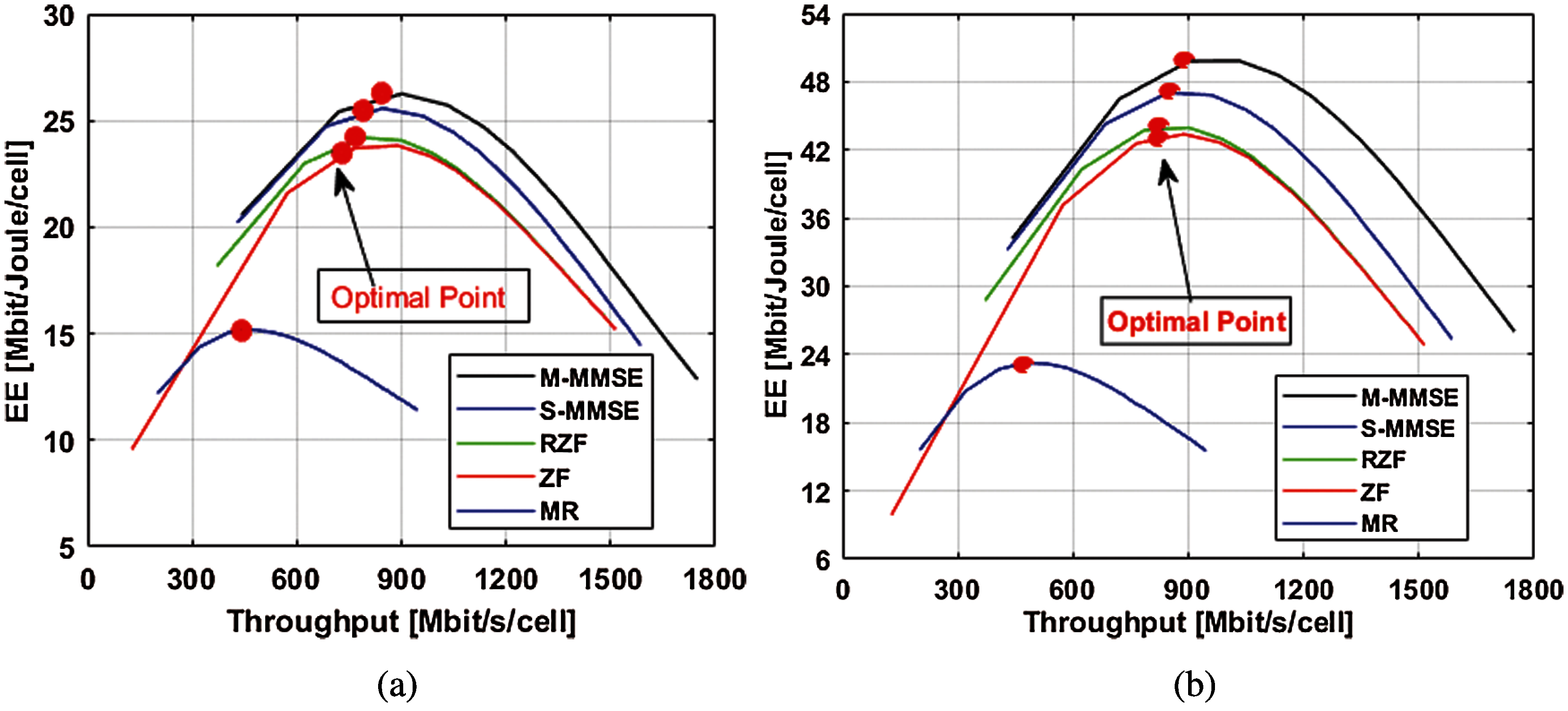
Figure 4: Throughput-EE tradeoff: (a) for the setting value-I, (b) for the setting value-II

The optimized results of the tradeoff between EE and throughput are shown in Tab. 7 with different combining and precoding schemes for UL and DL for all power consumption models separately. The final expression is given in Eq. (29) and two setting values are considered for the optimal tradeoff of EE-Throughput. The x-axis represents the throughput values in Mbit/s/km2 and the y-axis represents the EE in Mbit/Joule/cell. The power consumption models values in setting value-II as shown in Fig. 4b are half of the setting value-I as shown in Fig. 4a. Therefore, the EE is almost doubled as 27 is 52, 26 is 47, 24.5 is 43, 23.5 is 42, and 15 is 23 for M-MMSE, S-MMSE, RZF, ZF, and MR respectively (see Tab. 9). The above-mentioned values of EE are optimized value at throughput (Mbit/s/km2) of 890, 880, 850, 845, and 450 for different schemes. Our model indicates that reducing the total power consumption not only increases the EE but does not affect the throughput as in [25] it does.

In this article, we optimized the trade-off between EE and SE and throughput in the proposed massive MIMO system, and modeled UL and DL systems using the Wyner model. In the first step, we adopted two cell scenarios and calculated the expressions for uplink and downlink transmission based on the Wyner model. We proposed an optimization model for these two for both tradeoffs. We have calculated the parameters for selecting multiple antennas and selecting multiple users because these terms enhance SE and lower EE. The model verifies the optimization relationship of SE-EE through the approximation based on logarithmic function, and finds significant enlightenment to the results. The circuit power consumption is modeled to evaluate the trade-off between EE and throughput, while considering transmit power, circuit power consumed by the BS side hardware, encoding/decoding power, and digital signal processing power. In this regard, the UL and DL models for different combining and precoding schemes are used to formulate expressions for the BS in the massive MIMO network and calculate the total power consumption. We take and take M antennas and K UEs to calculate the throughput of M-MMSE, S-MMSE, RZF, ZF, MR combining and precoding schemes. The EE throughput trade-off result of power consumption model through the combining and precoding scheme is optimized. Moreover, it also has received the ability to fix the throughput by reducing the power consumption. The optimized trade-off results are verified in our model. The findings of this work assume that by optimizing EE to enhance SE and throughput in UL and DL transmissions, massive MIMO systems can be developed. We finally improve the EE. We optimize the choice of antenna and UE by evaluating actual power consumption.

In this paper, we considered both the uplink and downlink transmission while hardware and singular processing could be included to optimize the energy efficiency of massive MIMO systems in the future. However, massive MIMO encourages ultra-high frequency, so improving EE and SE are still open areas for further research.

Acknowledgement: This work was supported by the Deanship of Scientific Research at Prince Sattam bin Abdulaziz University, Saudi Arabia.

Conflicts of Interest: The authors declare that they have no conflicts of interest to report regarding the present study.

References

R. M. Asif, J. Arshad, M. Shakir, S. M. Noman and A. U. Rehman, “Energy efficiency augmentation in massive MIMO systems through linear precoding schemes and power consumption modeling,” Wireless Communications and Mobile Computing, vol. 1, no. 1, pp. 1–13, 2020.
E. G. Larsson, O. Edfors, F. Tufvesson and T. L. Marzetta, “Massive MIMO for next generation wireless systems,” IEEE Communications Magazine, vol. 52, no. 2, pp. 186–195, 2014.
J. Y. Jang, W. S. Lee, J. H. Ro, Y. H. You and H. K. Song, “Weighted gauss-seidel precoder for downlink massive MIMO systems,” Computers Materials and Continua, vol. 67, no. 2, pp. 1729–1745, 2021.
S. Cherry, “Edholm's law of bandwidth,” IEEE Spectrum, vol. 41, no. 7, pp. 58–60, 200
S. Bashir, M. H. Alsharif, I. Khan, M. A. Albreem, A. Sali et al., “Mimo-terahertz in 6G nano-communications: Channel modeling and analysis,” Computers Materials and Continua, vol. 66, no. 1, pp. 263–274, 2021.
J. Arshad, A. Rehman, A. U. Rehman, R. Ullah and S. O. Hwang, “Spectral efficiency augmentation in uplink massive MIMO systems by increasing transmit power and uniform linear array gain,” Sensors, vol. 20, no. 17, pp. 1–15, 2020.
A. Salh, L. Audah, Q. Abdullah, N. Shahida, M. Shah et al., “Energy-efficient low-complexity algorithm in 5G massive MIMO systems,” Computers Materials and Continua, vol. 67, no. 3, pp. 3189–3214, 2021.
P. Chan-Yeob, H. R. Jae, J. Y. Jang and S. Hyoung-Kyu, “An enhanced jacobi precoder for downlink massive MIMO systems,” Computers Materials and Continua, vol. 68, no. 1, pp. 137–148, 2021.
T. M. Nguyen and L. B. Le, “Joint pilot assignment and resource allocation in multicell massive MIMO network: Throughput and energy efficiency maximization,” in Proc. WCNC, LA, USA, pp. 393–398, 2015.
Y. Huang, S. He, J. Wang and J. Zhu, “Spectral and energy efficiency tradeoff for massive MIMO,” IEEE Transactions on Vehicular Technology, vol. 67, no. 8, pp. 6991–7002, 2018.
X. Chen, “Throughput multiplexing efficiency for MIMO antenna characterization,” IEEE Antennas and Wireless Propagation Letters, vol. 12, no. 1, pp. 1208–1211, 2013.
O. Onireti, F. Héliot and M. A. Imran, “On the energy efficiency-spectral efficiency trade-off in the uplink of CoMP system,” IEEE Transactions on Wireless Communications, vol. 11, no. 2, pp. 556–561, 20
F. Héliot, M. A. Imran and R. Tafazolli, “On the energy efficiency-spectral efficiency trade-off over the MIMO Rayleigh fading channel,” IEEE Transactions on Communications, vol. 60, no. 5, pp. 1345–1356, 2012.
O. Onireti, F. Heliot and M. A. Imran, “On the energy efficiency-spectral efficiency trade-off of distributed MIMO systems,” IEEE Transactions on Communications, vol. 61, no. 9, pp. 3741–3753, 2013.
O. K. Rayel, G. Brante, J. L. Rebelatto, R. D. Souza and M. A. Imran, “Energy efficiency-spectral efficiency trade-off of transmit antenna selection,” IEEE Transactions on Communications, vol. 62, no. 12, pp. 4293–4303, 2014.
H. Q. Ngo, E. G. Larsson and T. L. Marzetta, “Energy and spectral efficiency of very large multiuser MIMO systems,” IEEE Transactions on Communications, vol. 61, no. 4, pp. 1436–1449, 2013.
S. Mukherjee and S. K. Mohammed, “On the energy-spectral efficiency trade-off of the MRC receiver in massive MIMO systems with transceiver power consumption,” in Proc. IEEE GLOBECOM, Austin, USA, pp. 11404–11410, 2014.
S. Mukherjee and S. K. Mohammed, “Energy-spectral efficiency trade-off for a massive SU-mIMO system with transceiver power consumption,” in Proc. IICC, London, UK, pp. 1938–1944, 2015.
N. Achir, M. Debbah and P. Muhlethaler, “Massive MIMO cooperative communications for wireless sensor networks: throughput and energy efficiency analysis,” in Proc. ISPIMRC, Washington, pp. 590–594, 2014.
A. Salh, L. Audah, N. S. M. Shah and S. A. Hamzah, “Trade-off energy and spectral efficiency in a downlink massive MIMO system,” Wireless Personal Communications, vol. 106, no. 2, pp. 897–910, 2019.
B. Jiang, B. Ren, Y. Huang, T. Chen, L. You et al., “Energy efficiency and spectral efficiency tradeoff in massive MIMO multicast transmission with statistical CSI,” Entropy, vol. 22, no. 9, pp. 1–13, 2020.
L. You, J. Xiong, A. Zappone, W. Wang and X. Gao, “Spectral efficiency and energy efficiency tradeoff in massive MIMO downlink transmission with statistical CSIT,” IEEE Transactions on Signal Processing, vol. 68, no. 3, pp. 2645–2659, 2020.
S. M. Nimmagadda, “Optimal spectral and energy efficiency trade-off for massive MIMO technology: Analysis on modified lion and grey wolf optimization,” Soft Computing, vol. 24, no. 16, pp. 12523–12539, 2020.
N. Li, Y. Gao and K. Xu, “On the optimal energy efficiency and spectral efficiency trade-off of CF massive MIMO SWIPT system,” Journal on Wireless Communications and Networking, vol. 1, no. 1, pp. 1–10, 2021.
J. Choi, “On throughput improvement using immediate re-transmission in grant-free random access with massive mimo,” IEEE Transactions on Wireless Communications, vol. 19, no. 12, pp. 8341–8350, 2020.
E. Björnson, J. Hoydis and L. Sanguinetti, “Massive MIMO networks: Spectral, energy, and hardware efficiency,” Foundation Trends Signal Process, Hanover, USA, vol. 11, pp. 154–655, 2017. [Online]. Available: https://massivemimobook.com/wp/.
X. Li, E. Bjornson, S. Zhou and J. Wang, “Massive MIMO with multi-antenna users: When are additional user antennas beneficial?,” in Proc. ICT, Kuala Lumpur, Malaysia, pp. 464–471, 2017.
E. Björnson, L. Sanguinetti, J. Hoydis and M. Debbah, “Optimal design of energy-efficient multi-user MIMO systems: Is massive MIMO the answer?,” IEEE Transactions on Wireless Communications, vol. 14, no. 6, pp. 3059–3075, 2015.
E. Björnson, E. G. Larsson and M. Debbah, “Massive MIMO for maximal spectral efficiency: How many users and pilots should be allocated?,” IEEE Transactions on Wireless Communications, vol. 15, no. 2, pp. 1293–1308, 2016.

Computers, Materials & Continua DOI:10.32604/cmc.2022.020777
Article