Computers, Materials & Continua DOI:10.32604/cmc.2022.020793
Article

Data Wipe-Off Technique for Tracking Weak GPS Signals

Dah-Jing Jwo* and Sheng-Feng Chiu

Department of Communications, Navigation and Control Engineering, National Taiwan Ocean University, Keelung, 202301, Taiwan
*Corresponding Author: Dah-Jing Jwo. Email: djjwo@mail.ntou.edu.tw
Received: 08 June 2021; Accepted: 23 August 2021

In this paper, the data wipe-off (DWO) algorithm is incorporated into the vector tracking loop of the Global Positioning System (GPS) receiver for improving signal tracking performance. The navigation data, which contains information that is necessary to perform navigation computations, are binary phase-shift keying (BPSK) modulated onto the GPS carrier phase with the bit duration of 20 ms (i.e., 50 bits per second). To continuously track the satellite’s signal in weak signal environment, the DWO algorithm on the basis of pre-detection method is adopted to detect data bit sign reversal every 20 ms. Tracking accuracy of a weak GPS signal is decreased by possible data bit sign reversal every 20 ms to the predetection integration time (PIT) or integration interval. To achieve better tracking performance in weak signal environment, the coherent integration interval can be extended. However, increase of the integration interval lead to decrease of the tracking accuracy by possible data bit sign reversal every 20 ms to the integration interval. When the integration interval of the correlator is extended over 20 ms in low C/No levels, the navigation DWO algorithm can be employed to avoid energy loss due to bit transitions. The method presented in this paper has an advantage to continuously estimate the navigation data bit and achieve improved tracking performance. Evaluation of the tracking performance based on the various integration intervals for the vector tracking loop of a GPS receiver will be presented.

Keywords: Global positioning system (GPS); integration interval; data wipe-off; weak signal

1  Introduction

The Global Positioning System (GPS) [1–4] is a satellite-based navigation system [5,6] that provides a user with the proper equipment access to useful and accurate positioning information anywhere on the globe. Generally, the GPS receiver accomplishes the following two major functions: the tracking of pseudorange and the solution of navigation information. The signal tracking tries to adjust the local signal to have the same code phase with the received satellite signal. Each tracking channel measures the pseudorange and pseudorange rate, respectively, and then sends the measurements to the navigation processor, which solves for the user's position, velocity, clock bias and drift (PVT).

As the most vulnerable parts of a receiver, the carrier and code tracking loops play a key role in a GPS receiver. Traditional GPS receivers utilize the scalar tracking loop (STL) to track signals from different satellites independently. The STL consists of correlator, discriminator, loop filter, and numerically control oscillator (NCO) in each channel. The intermediate frequency (IF) signal is correlated with internally generated replica signal, and the output of correlator consists of in-phase (I) and quadrature-phase (Q) components via integrate-and-dump operation. The discriminator measures code phase error and carrier frequency error. These are passed to navigation filter and through loop filter to control NCO. Specifically, a delay lock loop (DLL) is used to track the code phase of the incoming pseudorandom code and a carrier tracking loop, such as a frequency lock loop (FLL) or a phase lock loop (PLL), is used to track the carrier frequency or phase. The tracking results from different channels are then combined to estimate the navigation solutions. The drawback of STL is that it neglects the inherent relationship between the navigation solutions and the tracking loop status. In that sense, a STL is more like an open loop system and provides poor performance when scintillation, interference, or signal outages occur.

The vector tracking loop (VTL) [7,8] provides a deep level of integration between signal tracking and navigation solutions in a GPS receiver. The VTL is a very attractive technique as it can provide tracking capability in degraded signal environment. In the VTL structure, all channels are processed together in one processor which is typically an estimator, such as the extended Kalman filter (EKF) [5]. In a VTL, each tracking loop update is also based on information from other tracking loops and results in several important improvements over the traditional STL, such as increased interference immunity, robust dynamic performance, and the ability to operate at low signal power and bridge short signal outages [9–13]. The conventional VTL based on the discriminator consists of correlator, discriminator and NCO, where the loop filter is removed in each channel. The discriminator outputs of each channel are passed to the navigation filter, which then provides feedback to NCO. The code loop NCO in STL is replaced by the estimated user positions, to control the update of the local code. The Doppler frequency and the pseudoranges are calculated from and can be used as the measurement of the navigation filter, usually an EKF. The navigation filter can be employed to estimate the navigation state PVT of the receiver. The error signals arise from the estimated user positions and the satellite positions calculated by the ephemeris. When one channel experiences interference or signal outages in the VTL, the information from other satellites can be used estimate the status of this channel. In general, it is known that the VTL based on the discriminator gives users an accurate position and Doppler frequency than the scalar vector tracking loop. The navigation processor in turn predicts the code phases.

The data wipe off (DWO), also referred to as the data bit wipe-off, or data wiping approach [14–16] can be utilized in the vector tracking loop of a GPS receiver to improve the tracking capability. The navigation data are binary phase-shift keying (BPSK) modulated onto the GPS carrier phase with a navigation data bit duration of 20 ms (i.e., 50 bit/s). Correlation integration intervals generally do not exceed the duration of a navigation data bit for those cases where the receiver operates in open sky conditions. Particularly, signal integration intervals from 10 to 20 ms are sufficient for open sky operations where the received signal C/No generally varies in the range from 32 to 50 dB-Hz. In a GPS receiver, the predetection integration time (PIT) should be less than the navigation data bit period. In order to increase the integration interval without loss of the correlation, one of the strategies is to remove the data bit of the GPS signal. Navigation DWO approach enable longer coherent integration times by removing the 50 Hz navigation data from the received signal. The DWO techniques are therefore employed to avoid energy loss that occurs due to bit transitions during the correlation integration. These techniques are most effective for GPS receivers that already have high anti-jam immunity and are not expected to significantly improve the tracking thresholds of most unaided GPS receivers. Different levels of signal quality, e.g., carrier-to-noise ratio (C/No), will influence I and Q values in the same coherent integration interval. Increase of integration interval will increase the anti-interference ability. In the case that C/No is low, it can improve the value by extending the coherent integration interval. Since the energy is decreased by the possible data bit sign reversal every 20 ms, thus the data wipe-off algorithm can be applied to avoid this situation.

This paper presents the vector tracking loop performance improvement of a GPS receiver using the data wipe-off techniques. The paper is organized as follows. In Section 2, preliminary background on the signal processing for the GPS receiver tracking loop is reviewed. The data wipe-off approach is introduced in Section 3. In Section 4, the navigation filter processing is introduced. In Section 5, simulation experiments are carried out to evaluate the performance and effectiveness. Conclusions are given in Section 6.

2  Signal Processing for the GPS Receiver Tracking Loop

A typical functional diagram of the GPS receiver signal processing is shown as in Fig. 1. The GPS signal is given by

s(t)=AC(t)D(t)cos⁡(ωt+θ)+n(t)(1)

where A is the amplitude, ω is the frequency at the antenna, θ is the Doppler frequency offset and n(t) is the thermal noise produced by the filter and amplifier plus the noise that entered the antenna.

Figure 1: Block diagram of the global positioning system (GPS) receiver signal processing

GPS receivers utilize an omni-directional antenna to receive the GPS signals. These are passed through a band-pass filter and low noise amplifier before being down-converted to an intermediate frequency (IF) by a mixer. Many GPS receivers use two down-conversions to reach baseband, where the analog signal is sampled and converted into digital in-phase and quadrature-phase channels by multiplication by sine and cosine versions of the local oscillator (mixing) frequency. Some receivers sample at an intermediate frequency, before down-converting to baseband. The down-conversion from RF to IF is achieved by mixing the RF signal with a local oscillator (LO), LO=2cos⁡(ω1t).

The signal at IF plus the noise at IF, and the upper band can be represented as

sIF(t)+nIF(t)+upperband=2cos⁡(ω1t)[s(t)+n(t)] (2)

which, after low pass filtering, yields

sIF(t)+nIF(t)=AC(t)D(t)cos⁡[(ω−ω1)t+θ)]+n(t)cos⁡[(ω−ω1)t)] (3)

The in-phase (I) component is realized by mixing sIF(t) and nIF(t) with an LO equal to LOI=2cos⁡(ω2t) and the quadrature-phase (Q) component is realized by mixing sIF(t) and nIF(t) with an LO equal to LOQ=2cos⁡(ω2t+900). The two LO’s are 90o phase-shifted with respect to one another. Due to the fact that ω−ω1−ω2=0, the in-phase and quadrature-phase components

Is(t)=A2C(t)D(t)cos⁡(θ);Qs(t)=−A2C(t)D(t)sin⁡(θ) (4)

with the noises in the in-phase and quadrature-phase components, respectively, given by

In(t)=12n(t);Qn(t)=−12n(t) (5)

Signals sampled using analog-to-digital conversion, the in-phase and quadrature-phase components, respectively, at time, tk,k=0,1,2,…, can be written as

Is,k=A2CkDkcos⁡(θk);Qs,k=−A2CkDksin⁡(θk) (6)

with the corresponding noises

In,k=12nk;Qn,k=−12nk (7)

The Doppler shift can be removed from the signal via phase rotation, which is achieved in a carrier tracking loop via a numerically controlled oscillator (NCO), which creates cosine and sine components that operate at a reference phase offset θrD. Let θrD,k be the reference phase offset at time tk, then the in-phase component of the signal is

ID,k=A2CkDkcos⁡(θk−θrD,k);QD,k=A2CkDksin⁡(θk−θrD,k) (8)

which can be multiplied with the digital reference C/A code at time tk, Crp,k.

IC,k=A2CkCrp,kDkcos⁡(θk−θrD,k);QD,k=A2CkCrp,kDksin⁡(θk−θrD,k) (9)

The expected value of the accumulated correlated in-phase signal component is shown to be

IA,k=E[∑k=1MIC,k]=A2Di∑k=1ME[CkCrp,k]cos⁡(θk−θrD,k)=A2DiR(τ)∑k=1Mcos⁡(θk−θrD,k) (10)

where R(τ)=E[CkCrp,k] represents the normalized autocorrelation function. Assuming the navigation data Di remains unchanged (+1 or −1) within the integration interval T, the relation holds: T=MΔtk, where M is the number of samples summed within epoch T, which is 1 ms for the length of the C/A code sequence. Using the linear approximation θk−θrD,k≈2πfit+Δθi, if the kth sample point is the endpoint of the kth subinterval for both summations, then the summation has the form

∑k=1Mcos⁡(θk−θrD,k)≈1Δtk∫0Tcos⁡(2πfit+Δθi)dt (11)

An approximation of the accumulated in-phase signal component can be shown to be

IA,k=A2DiR(τ)MT∫0Tcos⁡(2πfit+Δθi)dt (12)

The integral in the above equation can be approximated and simplified as follow

∫0Tcos⁡(2πfit+Δθi)dt=12πfisin⁡(2πfit+Δθi)|0T=12πfi[sin⁡(2πfiT+Δθi)−sin⁡(Δθi)]=12πfi[2sin⁡(2πfiT+Δθi−Δθi2)cos⁡(2πfiT+Δθi+Δθi2)]=1πfisin⁡(πfiT)cos⁡(πfiT+Δθi) (13)

and the accumulated in-phase signal component IA,k may be written as

IA,k=A2MDiR(τ)sin⁡c(πfiT)cos⁡(πfiT+Δθi) (14)

Assuming the noise IC,n is a zero-mean white Gaussian noise

IA,n=E[∑k=1MIC,n]=∑k=1ME[IC,n]=0 (15)

with variance

σn2=E[(∑k=1MIC,n)2]=E[(1Δtk∫0TIc,ndt)2]=E[(1ΔtkIc,nT)2]=(TΔtk)2E[Ic,n2] (16)

Since the Fourier transform of the two-sided bandwidth Gaussian white noise is N02T, we have

E[Ic,n2]=∫01TN02dt=N02T (17)

with the variance given by

σn2=T2Δtk2N0=M2ΔtkN0 (18)

In order to normalize the noise variance, the in-phase component is multiplied by the factor

Since S=A22 represents the average power of a GPS signal, the ith accumulated in-phase component at time tk is given by

Ii=2ΔtkMN0(IA,k+IA,n)=2SN0TDiR(τ)sin⁡c(πfiT)cos⁡(πfiT+Δθi)+nI (19)

Similarly, the ith accumulated quadrature-phase component at time tk may be written as

Qi=2SN0TDiR(τ)sin⁡c(πfiT)sin⁡(πfiT+Δθi)+nQ (20)

The signal energy for a given pair of accumulated I and Q is computed as I2+Q2.

3  The Data Wipe-Off Approach

Correlation integration intervals generally do not exceed the duration of a navigation data bit (20 ms) for those cases where the receiver operates in open sky conditions. If the integration interval is extended longer than the period of data bit, the loss of the correlation values will occur due to the data bit transmission. A DWO algorithm is commonly employed for performance improvement on the basis of pre-detection method to detect data bit sign reversal every 20 ms.

Employed to extend the integration interval of the correlator, there are two commonly used DWO algorithms: (1) an energy-based bit estimation algorithm; (2) a carrier phase discriminator based algorithm, to remove the data bit in I and Q correlation values. The DWO method in this paper utilizes the energy-based bit estimation algorithm, shown as in Fig. 2. The parameter D^k is the estimated data bit and k is the time epoch. The data bit of correlator output is stripped by estimated data bit. This method removes the navigation data bit in I and Q values and can prevent the estimation state from divergence due to the navigation data bit transition.

For illustration purpose, we assume that the correlator integration interval is 100 ms, which is five times of data bit transition. The initial point of navigation data bit is known due to acquisition process. We start tracking from this point. For the example of 100 ms interval, there are five 20 ms accumulated I values and five 20 ms accumulated Q values. The signal energy for a given pair of accumulated I and Q is computed as I2+Q2. It should be noted that the energy computation is insensitive to the sign polarity of a bit combination, i.e., bit combinations with an opposite sign (e.g., [1 1 −1 −1 −1] and [−1 −1 1 1 1]) have the same signal energy. The maximum energy bit combination is thus computed for the bit combinations where no opposite sign combinations are present. It therefore contains 16 possible bit combinations bit combinations, represented by the B matrix.

B=[111111111−1111−1−1⋮⋮⋮⋮⋮1−1−1−1−1]16×5 (21)

Figure 2: Block diagram for the data wipe-off (DWO) algorithm

Each row of B matrix corresponds to a particular bit combination. Energy computation is performed through a single matrix multiplication:

[I0.1s,1⋮I0.1s,16]=B⋅[I0.02s,1⋮I0.02s,5]; [Q0.1s,1⋮Q0.1s,16]=B⋅[Q0.02s,1⋮Q0.02s,5] (22)

where I0.02s,j,Q0.02s,j,j=1,…,5 are I and Q accumulated over the duration of the jth data bit inside the 100 ms tracking integration interval. Compute the sum of squares of I0.1s and Q0.1s

[E1⋮E16]=[I0.1s,12⋮I0.1s,162]+[Q0.1s,12⋮Q0.1s,162] (23)

A sign combination and a sequence of bit combinations that maximize the signal energy over tracking integration interval are chosen:

Emax=maxk(Ek),k=1,⋯,16 (24)

The discriminator input signals are as follow:

I0.1s=I0.1s,kmax,Q0.1s=Q0.1s,kmax (25)

As an example, the energy of possible sequential combinations is provided in Fig. 3, for which energy plots for two of the channels are shown. See [16] for further detailed information about the method.

4  Navigation Filter Processing

The GPS VTL differs from the traditional STL in that the task of navigation solutions, code tracking and carrier tracking loops for all satellites are combined into one loop. The central part of a VTL is an estimator, which is usually a Kalman filter to provide an estimation of signal parameters for all satellites in view and user PVT solutions based on both current and previous measurements from all satellites. The discriminator outputs of each channel are passed to the navigation filter. The DWO method using carrier phase discriminator is incorporated into the GPS VTL to remove the navigation data bit in I and Q correlation values. Fig. 4 shows the system configuration of the vector tracking loop with DWO mechanism.

Figure 3: Energy of possible sequential combinations

Figure 4: System configuration of the vector tracking loop (VTL) with DWO mechanism

The nonlinear filters deal with the case governed by the nonlinear stochastic difference equations:

where the state vector xk∈ℜn, process noise vector wk∈ℜn, measurement vector zk∈ℜm, and measurement noise vector vk∈ℜm. Both the vectors wk and vk are zero mean Gaussian white sequences having zero cross-correlation with each other:

E[wkwiT]=Qkδki;E[vkviT]=Rkδki;E[wkviT]=0; for all i and k

where Qk is the process noise covariance matrix, and Rk is the measurement noise covariance matrix.

When selecting EKF as the navigation state estimator in the GPS receiver, using b and d to represent the GPS receiver clock bias and drift, the differential equation for the clock error is written as b˙=d+ub and d˙=ud, where ub∼N(0,Sf) and ud∼N(0,Sg) are independent Gaussianly distributed white sequences. The dynamic process of the GPS receiver in lower dynamic environment can be represented by the PV (Position-Velocity) model, where three position states, three velocity states, and two clock states are involved, so that the state to be estimated is a 8×1 vector.

Information for the receiver dynamic includes the pseudorange, range-rate and Doppler frequency, discussed as follows. Mathematical model for the pseudorange observable is given by

and the satellite-to-antenna range rate is given by

where i is the receiver channel number, bk and b˙k are the clock bias and drift, respectively. The Doppler frequency can be represented by

fi,k=−ρ˙i,k/λφ (26)

The code phase error (in chip) can be written as

Δτi,k=ρi,k−ρ^i,k−λτ (27)

and the Doppler frequency error (in Hz) can be found as

Δfi,k=fi,k−f^i,k−=−ρ˙i,k−ρ˙^i,k−λφ (28)

where λφ is the carrier wave length, and λτ is the code chip length. The carrier phase error (in rad) is given by

Δφi,k=πΔfi,kT+φ0 (29)

where T is the code integration interval and φ0 is the initial phase. The correlator accumulator outputs for I and Q arms, respectively, are given by

IE/P/L=ADR(Δτ+δj)sin⁡c(πΔfT)cos⁡(Δφ)+nI (30)

and

QE/P/L=ADR(Δτ+δj)sin⁡c(πΔfT)sin⁡(Δφ)+nQ (31)

In the above equation, δj is the early/prompt or prompt/late correlator spacing, D is the navigation data, and the correlation function R(τ) takes the form

R(τ)={1−|τ|0|τ|≤1|τ|>1 (32)

The normalized amplitude of the GPS signal amplitude As is given by A=As/σnoise=2TS/No, where σnoise is the standard deviation of the noise. The discriminators cover the code and carrier frequency. The code phase error based on the discriminator is obtained using

Δτ^i,k=1(IE,k2+QE,k2−IL,k2+QL,k2)2(IE,k2+QE,k2+IL,k2+QL,k2) (33)

where Δτ^i,k represents the estimation of the code phase error. The error of carrier frequency from the discriminator output is evaluated using

Δf^i,k=ATAN2(dot,cross)(tk−tk−1) (34)

where the notations dot=IP,k⋅IP,k−1+QP,k⋅QP,k−1 and cross=IP,k⋅IP,k−1−QP,k⋅QP,k−1. The measurements used for navigation Kalman filter include the predicted pseudorange error (Δρ^k) and range-rate error (Δρ˙^k) are given by

Δρ^k=λτ⋅Δτ^k (35)

and

Δρ˙^k=−λφ⋅Δf^k (36)

respectively.

If the measurement equation for the navigation filter is composed of pseudorange and range-rate observables, zk=[ρk1⋯ρkiρ˙k1⋯ρ˙ki]T the measurement matrix Hk is an (n×8) matrix

where (hx,ihy,ihz,i) is the line-of-sight unit vector.

5  Results and Discussion

Several tests have been carried out for confirmation of the effectiveness and justification of the performance. Simulation was conducted using a personal computer. The computer codes were developed by the authors using the Matlab® software. The commercial softwares Satellite Navigation Toolbox (SatNav) [17] and Inertial Navigation System Toolbox (INS) [18] by GPSoft LLC were employed. The trajectory of vehicle was generated by Inertial Navigation Toolbox software and the information related to satellite signals used for navigation processing was generated by the Satellite Navigation Toolbox software. The simulation scenario is as follows. The experiment was conducted on a simulated vehicle trajectory originating from the position of (0, 0, 0) m location in the local tangent East-North-Up (ENU) frame. Fig. 5 shows the test trajectory and the skyplot configuration during the experiment. Tab. 1 presents description of the carrier-to-noise ratio for the visible satellites in simulation, where the C/No varies from 25 to 47 dB-Hz.

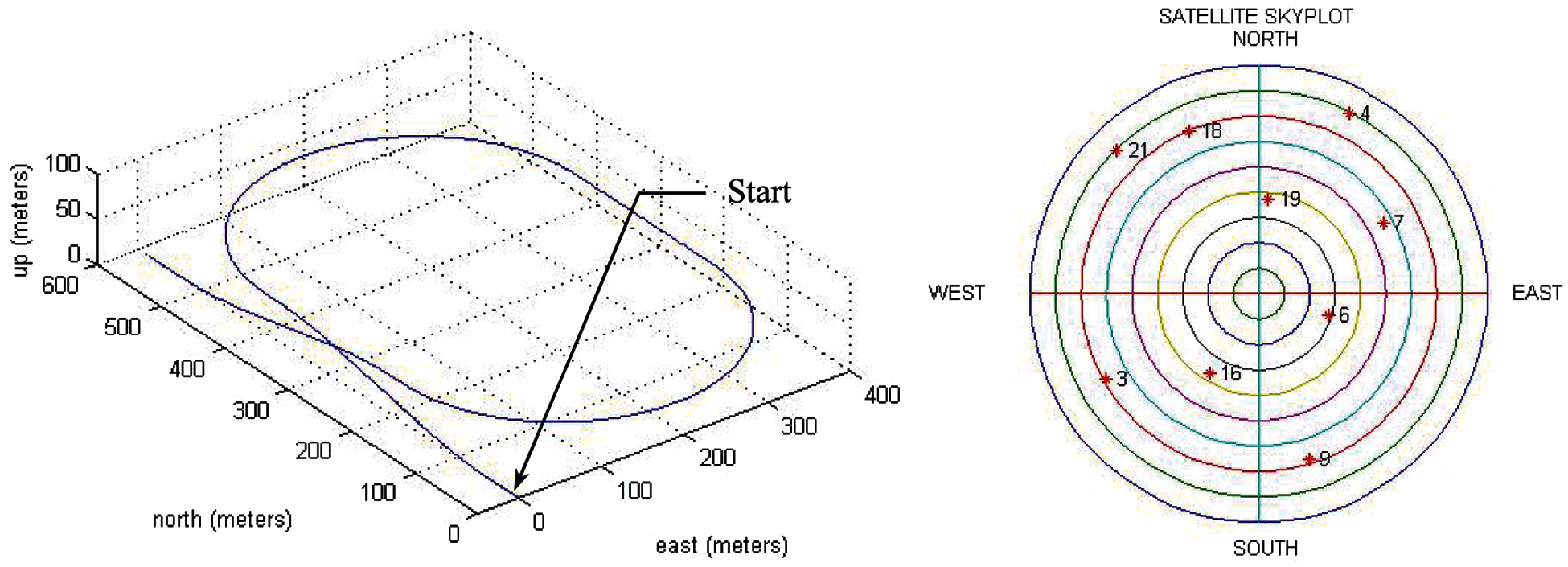
Figure 5: The three dimensional test trajectory and the skyplot configuration during theexperiment

The following discussion presents performance comparison for the design with DWO algorithm involved when various integration intervals are involved. Figs. 6 and 7 present the results in three of the channels (i.e., PRNs 3, 6 and 9) for the case of 20 ms integration interval employed. Fig. 6 presents the code phase and Doppler frequency errors in three of the channels tracking errors for the code phase and Doppler frequency errors in three of the channels, while Fig. 7 shows the corresponding energies for the in-phase components. It should be noticed that the three sets of energies for the three channels for the quadrature-phase components are very close each other and almost not distinguishable and therefore only the in-phase energies are compared.

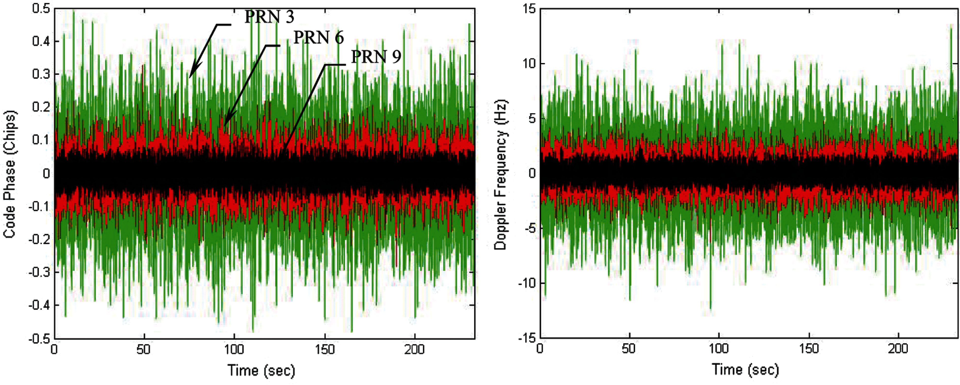
Figure 6: Tracking errors for the code phase and Doppler frequency-20 ms integration interval

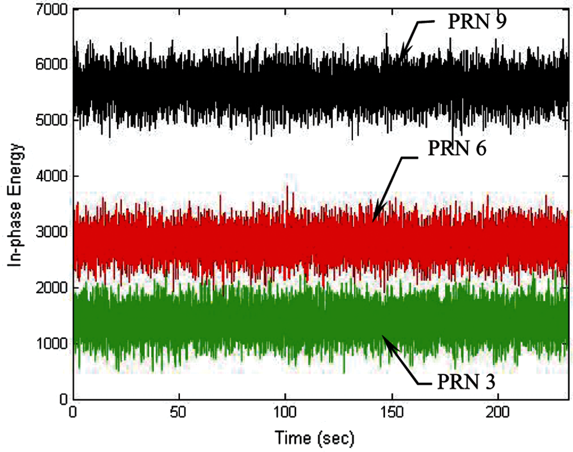
Figure 7: Energies for the in-phase component in three of the channels-20 ms integration interval

To overcome the problem of loss of lock when the signal is weak, the DWO approach is applied to mitigate the influence of navigation data on I and Q. Increase of the integration interval can effectively increase the energy in the I arm. Figs. 8 and 9 present the results for the cases when the integration interval is increased to 60 ms. In such case, the tracking errors for the code phase and Doppler frequency errors are shown in Fig. 8, followed by the energies for the in-phase component in three of the channel shown in Fig. 9. It can be seen that tracking accuracy was remarkably improved when longer integration interval was adopted. Further increase of the integration interval from 60 to 100 ms is discussed with the results shown in Figs. 10 and 11. Fig. 10 presents the tracking errors for the code phase and Doppler frequency, while Fig. 11 shows the corresponding energies for the in-phase component in three of the channels. Under the low-quality signal environments, it is very useful for accuracy improvement by extending the integration interval.

Figure 8: Tracking errors for the code phase and Doppler frequency-60 ms integration interval

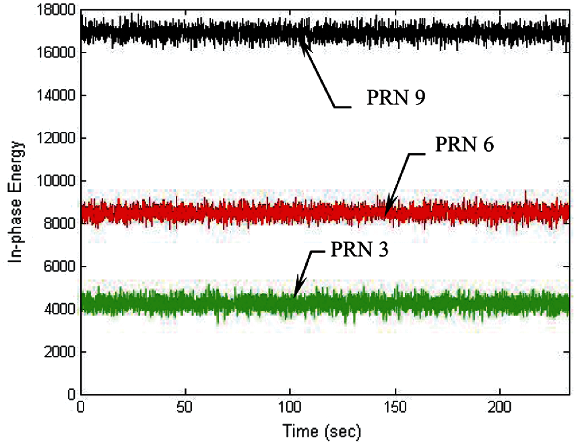
Figure 9: Energies for the in-phase component in three of the channels-60 ms integration interval

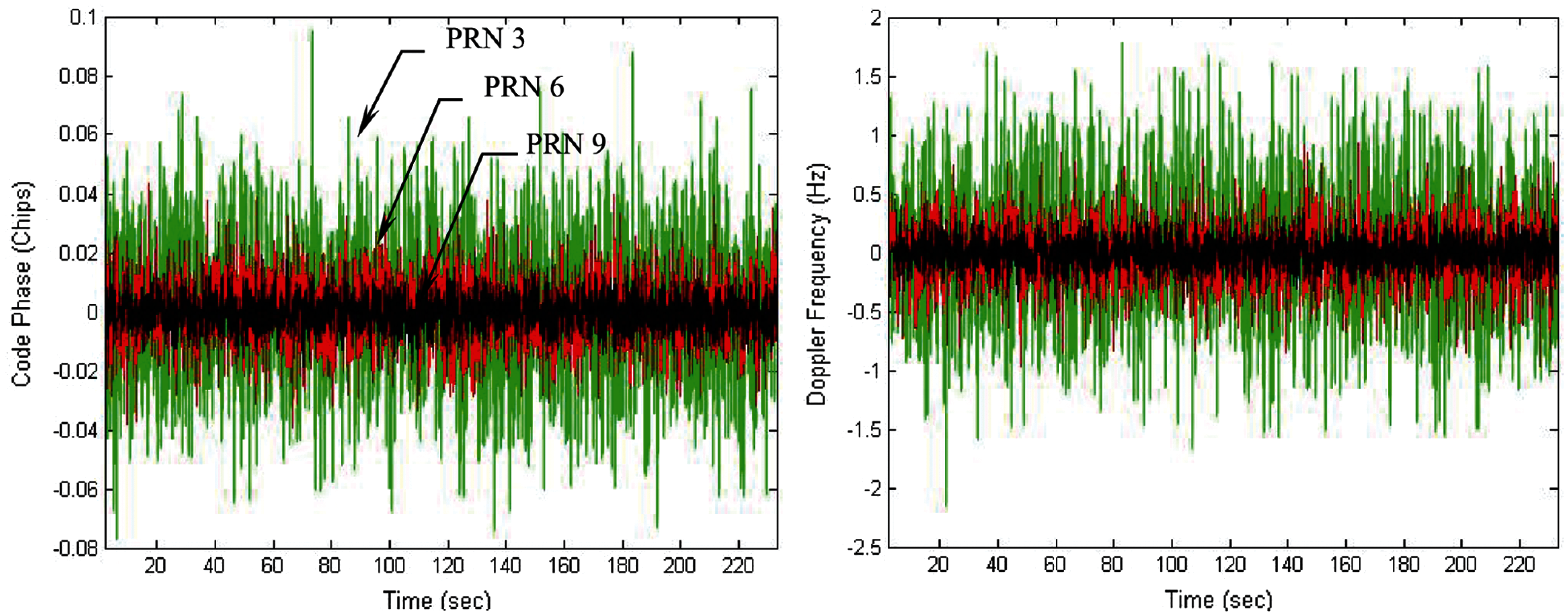
Figure 10: Tracking errors for the code phase and Doppler frequency-100 ms integration interval

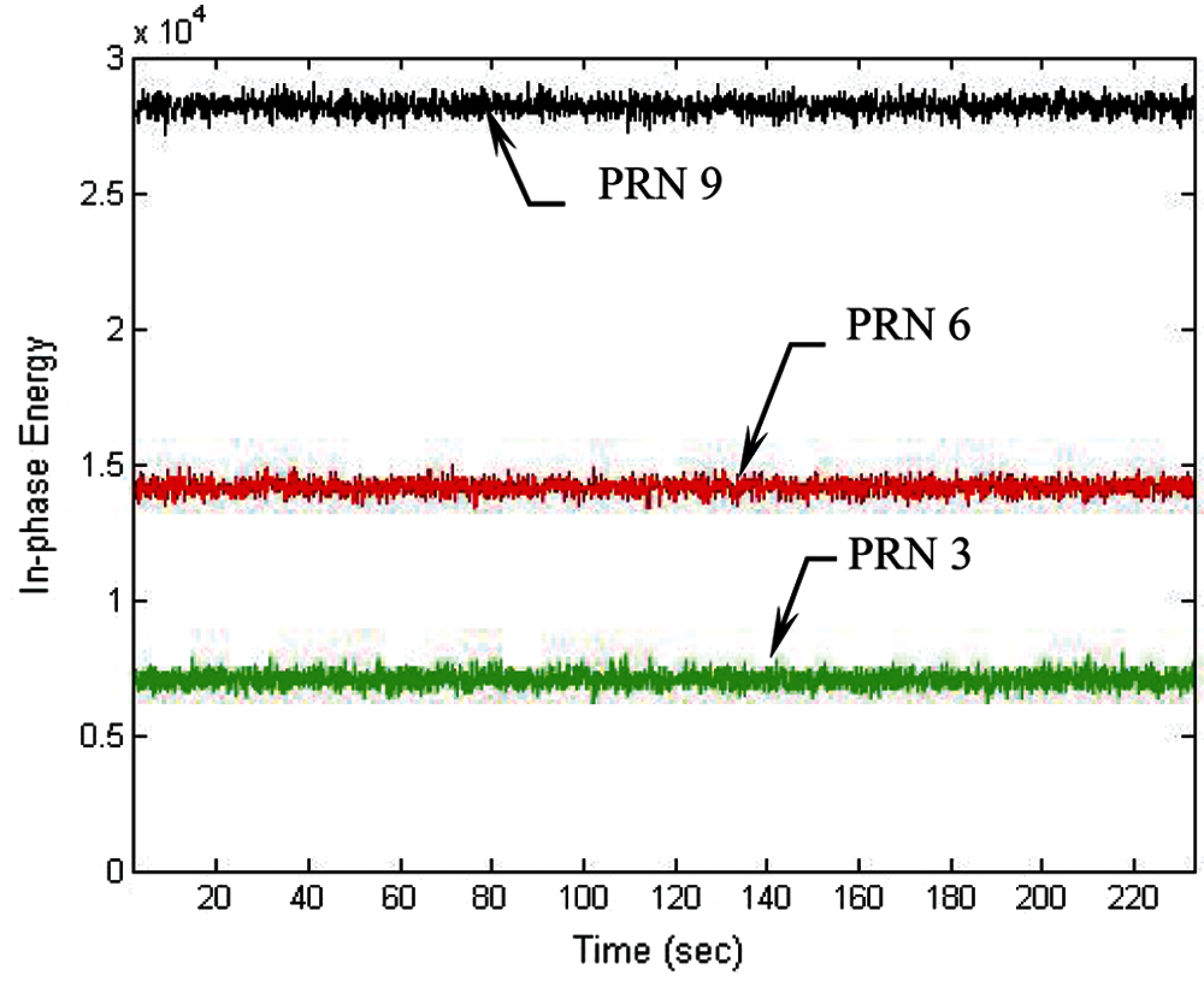
Figure 11: Energies for the in-phase component in three of the channels-100 msintegration interval

As an example on the weak signal environment, the performance for PRN 3 is illustrated. Fig. 12 provides code phase and Doppler frequency errors for PRN 3, where the integration intervals used were 20, 60 and 100 ms, respectively. Fig. 13 gives the energy for the in-phase components for various integration intervals. With higher C/No, the energy in the I arm becomes higher, and the discriminator provide better tracking accuracy. Position errors for the VTL for various integration intervals are presented in Fig. 14 and the error statistics are summarized in Tab. 2.

Figure 12: Code phase and Doppler frequency errors for PRN 3

Figure 13: Energies for the in-phase components for various integration intervals for PRN 3

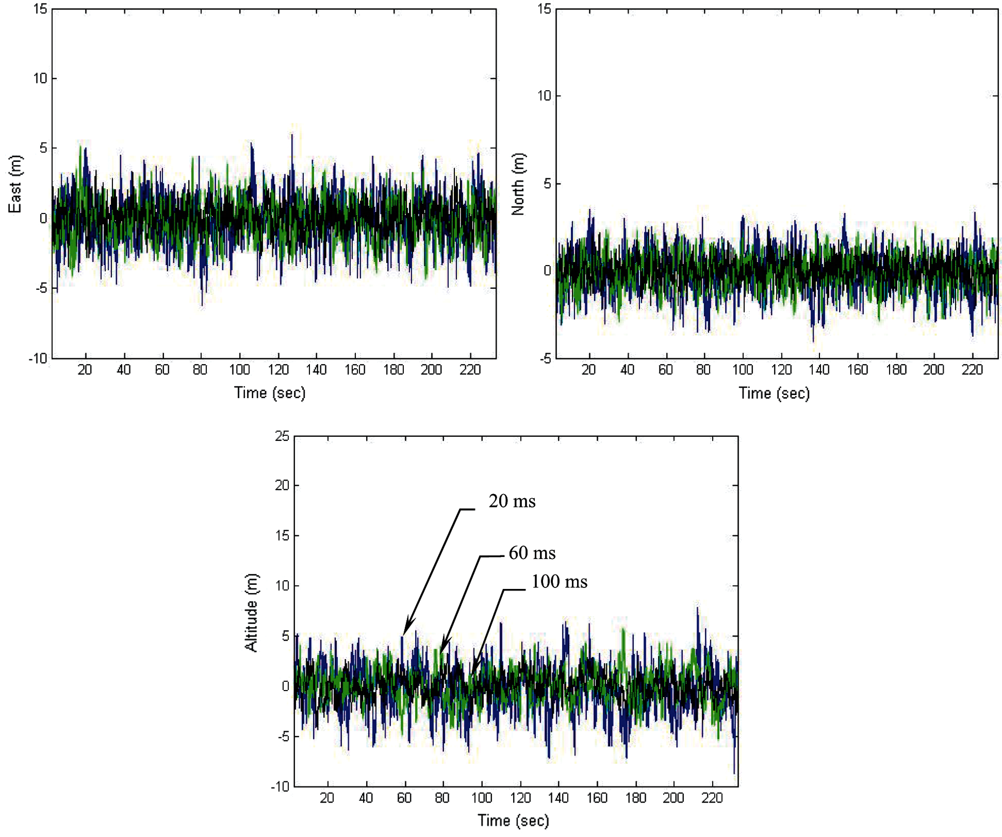
Figure 14: Position errors for the VTL for various integration intervals

6  Conclusions

This paper employs the data wipe-off algorithm for the GPS receiver to improve the tracking and navigation accuracy. Conventional GPS receivers use scalar tracking loop and satellite signals from each channel are processed independently. On the vector tracking loop, signals in these channels can be shared with each other for improved tracking performance under the low-quality signal environment. The accumulated energy might be decreased by the possible data bit sign reversal every 20 ms to the integration interval. To resolve the problem, a data wipe off algorithm is presented on the basis of pre-detection method to detect data bit sign reversal every 20 ms. The data wipe-off method based on the energy-based bit estimation algorithm is employed to avoid energy loss due to bit transitions. The integration interval of the correlator can be extended over 20 ms in low C/No levels.

Examples have been presented for illustration. The method presented in this paper has an advantage to continuously estimate the navigation data bit and achieves improved tracking performance. Tracking accuracy of a weak GPS signal is increased by extending the coherent integration interval. In the weak signal environment, it is especially useful by extending integration interval. The coherent integration interval has been extended over 20 ms. Position errors based on various integration intervals, including 20, 60 and 100 ms, are presented. The results show that the tracking accuracy increases when longer integration interval is utilized. The simulation results show that the vector tracking loop with data wipe-off module enables improved tracking and navigation accuracy and demonstrates good potential in dealing with degraded signals.

Funding Statement: This work has been partially supported by the Ministry of Science and Technology, Taiwan [Grant numbers MOST 101-2221-E-019-027-MY3 and MOST 109-2221-E-019-010].

Conflicts of Interest: The authors declare that they have no conflicts of interest to report regarding the present study.

This work is licensed under a Creative Commons Attribution 4.0 International License, which permits unrestricted use, distribution, and reproduction in any medium, provided the original work is properly cited.