DOI:10.32604/cmc.2022.020847
| Computers, Materials & Continua DOI:10.32604/cmc.2022.020847 | |
| Article |
IRKO: An Improved Runge-Kutta Optimization Algorithm for Global Optimization Problems
1Department of Computer Science and Engineering, Kongu Engineering College, Perundurai, 638060, Tamil Nadu, India
2Department of Electrical & Electronics Engineering, Dayananda Sagar College of Engineering, Bengaluru, 560078, Karnataka, India
3Rajasthan Rajya Vidyut Prasaran Nigam, Sikar, 332025, Rajasthan, India
4Mechanical Engineering Department, College of Engineering, King Khalid University, Abha, 61421, Saudi Arabia
5Mechanical Engineering Department, Faculty of Engineering, Kafrelsheikh University, Egypt
6Clean and Resilient Energy Systems (CARES) Laboratory, Texas A&M University, Galveston, 77553, TX, USA
7College of Arts and Sciences, Prince Sattam bin Abdulaziz University, Wadi Aldawaser, 11991, Saudi Arabia
*Corresponding Author: Kottakkaran Sooppy Nisar. Email: n.sooppy@psau.edu.sa
Received: 11 June 2021; Accepted: 22 July 2021
Abstract: Optimization is a key technique for maximizing or minimizing functions and achieving optimal cost, gains, energy, mass, and so on. In order to solve optimization problems, metaheuristic algorithms are essential. Most of these techniques are influenced by collective knowledge and natural foraging. There is no such thing as the best or worst algorithm; instead, there are more effective algorithms for certain problems. Therefore, in this paper, a new improved variant of a recently proposed metaphorless Runge-Kutta Optimization (RKO) algorithm, called Improved Runge-Kutta Optimization (IRKO) algorithm, is suggested for solving optimization problems. The IRKO is formulated using the basic RKO and local escaping operator to enhance the diversification and intensification capability of the basic RKO version. The performance of the proposed IRKO algorithm is validated on 23 standard benchmark functions and three engineering constrained optimization problems. The outcomes of IRKO are compared with seven state-of-the-art algorithms, including the basic RKO algorithm. Compared to other algorithms, the recommended IRKO algorithm is superior in discovering the optimal results for all selected optimization problems. The runtime of IRKO is less than 0.5 s for most of the 23 benchmark problems and stands first for most of the selected problems, including real-world optimization problems.
Keywords: Engineering design; global optimization; local escaping operator; metaheuristics; Runge-Kutta optimization algorithm
The term “optimization” relates to determining the best values of different system components to complete the systems engineering at the lowest possible price. In machine learning and artificial intelligence, practical applications and problems are typically constrained, unconstrained, or discrete [1,2]. As a result, finding the best solutions using standard numerical programming approaches is difficult. Numerous optimization methods have been established in recent years to enhance the performance of various systems and reduce computing costs. Conventional optimization techniques have several flaws and restrictions, such as convergence to a local minimum and an undefined search space. Many novel optimization approaches have been presented in recent years to address such flaws. Most systems are nonlinear and require advanced optimization techniques to be evaluated. Mathematical optimization techniques are often inspired by findings in nature. Such algorithms produce random solutions inside the search space and keep making improvements until these results converge to probable global optimums. Every metaheuristic algorithm does have its settings that influence the optimization process [3–6]. In general, each metaheuristic algorithms share common characteristics, such as the search strategy, which itself is divided into two sections, one of which is known as diversification and the latter of which has been known as intensification. The first phase of the algorithm creates random variables in the initial phase to explore potential search space locations. The optimization approach attempts to discover the best result from the search space in the second phase. An excellent optimization algorithm must balance the exploitation and exploration phase to prevent entrapment at the local minima. The highest complications of such algorithms are in having an exact balance between exploitation and exploration phases to avoid trap from local minima and still enhance the solution accuracy previously obtained [7–9]. As per the discussion by [10], there are no bad or good among the various optimization techniques, but one more suitable for a certain problem, that is, still has a gap for developing new optimization techniques.
The authors want to provide a more efficient and successful method, and hence this paper proposes an Improved Runge-Kutta Optimization (IRKO) algorithm, a revolutionary metaphor-free optimization method. The suggested IRKO is formulated from the basic version of the RKO algorithm [11], and it employs a particular slope computation ideology based on the Runge-Kutta technique as a search engine for optimization problems. To improve the solution quality of the IRKO, the Local Escaping Operator (LEO) [12] is integrated with the RKO. To thoroughly demonstrate the robustness and efficacy of the IRKO, a set of twenty-three classical benchmarks and three constrained engineering problems is employed.
The paper has been organized as follows: Section 2 confers the backgrounds of metaheuristic algorithms related works, and Section 3 discusses the formulation of the IRKO algorithm employing RKO and LEO concepts. Section 4 demonstrates the numerical simulation results on classical benchmark functions and real-world problems. Section 5 concludes the paper.
Metaheuristic algorithms are divided into four categories relying on the motivation for its development: (i) swarm behaviors, (ii) natural behaviors, (iii) human behaviors, and (iv) physics concepts.
2.1 Swarm Intelligence Algorithms
Swarms can inspire natural and social phenomena. Several algorithms have been developed and presented by many researchers. Particle Swarm Optimization (PSO) is a common approach derived from the natural behavior of swarming particles [13]. Each particle can be updated as per the local positions and its global best position. The PSO addresses various challenges, such as solving global optimization problems, power systems, power electronics, feature selection, image segmentation, electric vehicles, data clustering, and much more. Ant foraging behavior inspires the Ant Colony Optimization (ACO) algorithm [14]. The ants release pheromone on the earth naturally to ensure the colony members choose the ideal path. It has been employed in several optimization problems, as stated earlier. Firefly Algorithm (FA) is based on the flashing strobe of fireflies in the sea [15]. It was well-received and implemented in many applications, such as feature selection, data clustering, mechanical systems, power systems, and other optimization challenges. The Artificial Bee Colony (ABC) algorithm is designed to mimic the activity of a honey bee [16]. It contains three groups: bees who are working, onlookers that are observing, and Scouters who are searching for food. The ABC algorithm has numerous applications, such as global optimization, job shop scheduling, wireless sensor network, image segmentation, etc. In addition, various algorithms proved to be effective for optimization problems, such as Gray Wolf Optimizer (GWO) [17], Harris-Hawks Optimizer (HHO) [18], Whale Optimization Algorithm (WOA) [19], Aquila optimizer [20], slime mold algorithm [21], marine predator algorithm [22], equilibrium optimizer [23], salp swarm optimizer [24], etc.
Numerous techniques presented in the literature use natural evolution's inherent characteristics to address optimization challenges. Examples of several evolutionary algorithms are as follows. The Genetic Algorithm (GA) is the most often used evolutionary technique [25]. The GA was invented after Darwinian evolution. It has gained much interest and has been widely applied in various applications, such as power systems, power electronics, electric vehicles, facial recognition, network anomaly detection, and scheduling problems. The authors of [26] demonstrate differential evolution algorithm in 1997, and it is considered to be an effective algorithm for many real-world applications. For instance, text classification, global optimization, image classification, parallel machine scheduling, power systems, smart grid, microgrid, wireless sensor networks, etc. Other famous algorithms, called biogeography-based optimizer [27], sunflower optimization [28], invasive tumor growth [29], etc., have been proven in numerous optimization tasks.
Researchers presented numerous metaheuristic algorithms by mimicking real human actions. Teacher Learning-Based Optimizer (TLBO) is inspired by teachers’ impact on their student's achievement [30]. Various problems have been solved by applying TLBO, including problems with constraints. Socio-evolution learning optimizer is developed by mimicking the human's social learning grouped as families in a social environment. Additional human-based algorithms, such as Hunger Games Search Optimizer (HGSO) [31], political optimizer [32], harmony search [33], Jaya algorithm [34], Rao algorithm [35], etc., are some of the best algorithms for solving optimization problems.
To provide alternatives to optimization problems, physics-based algorithms rely on physical laws. Big Bang-Big Crunch is a prominent MH algorithm inspired by the universe's development, and it has been applied in various applications, such as data clustering, global optimization, and various engineering design problems. The law of gravity and mass relations inspired the Gravitational Search Algorithm (GSA) [36]. It has also gotten much press and has been utilized to enhance and address various applications, such as global optimization, feature selection, image segmentation, and so on, which are only a few examples. The multi-verse optimizer is based on physics’ multi-verses hypothesis. It has handled various problems, including global optimization, forecasting, power systems, feature selection, etc. Other physics-based algorithms, such as the Sine-Cosine Algorithm (SCA) [37], Ion-Motion Optimizer (IMO) [38], and equilibrium optimizer [23], are few best algorithms for solving optimization problems.
In general, population-based optimization algorithms begin procedures by randomly selecting candidate solutions. Such solutions are improved significantly by the algorithms and iteratively assessed against a specified fitness function, which is the basis of any algorithms. Due to the stochastic nature, obtaining an optimal or near-optimal solution in a single run is not sure. However, many random solutions and evolutionary rounds increase the possibility of discovering the global optima for the given problem. Regardless of the differences in algorithms used in metaheuristic approaches, the optimization process may be separated into two distinct phases: exploration and exploitation. This refers to the broad scope of searching by employing several solutions provided by the algorithms to circumvent search difficulties.
3 Improved Runge-Kutta Optimization (IRKO) Algorithm
Firstly, this section discusses the concepts of the RKO algorithm and LEO and then extends the discussion to the development of the IRKO algorithm using RKO and LEO.
3.1 Runge-Kutta Optimization (RKO) Algorithm
The RKO algorithm is characterized by the absence of metaphors and strict attention to the underlying mathematical structures [11]. It is inappropriate to describe the population-based technique's framework using metaphors, as doing so conceals the basis of the mathematics that power the optimizers. Thus, RKO was established considering the logic of the Runge-Kutta (RK) approach and the growth of a population of individuals. The RK employs a special formulation to handle ordinary differential equations. The fundamental premise of RKO is based on the RK method's suggested estimated gradient. The RKO employs that as a method of exploring the search space to form a set of rules. The initialization phase is the first step in algorithms, and this phase of the RKO is similar to other population-based algorithms. This section discusses only the main mathematical formulation RKO algorithm.
The solution space is divided into regions, with random solutions placed in each region. A set of search solutions are then placed into the various regions, and a balance between exploitation and exploration is established. To identify the search strategy in the RKO algorithm, the RK4 approach was applied. Thus, the search mechanism (SM) in RKO is represented in Eq. (1).
where k1, k2, k3, k4 are coefficients of the first-order derivative by the RK and
The RKO algorithm starts the procedure with a random population (solutions). Every time around, the solutions’ positions are updated by the RK method. RKO employs a solution and the search mechanism generated using the Runge-Kutta approach. To offer exploration and exploitation search, Eq. (3) is utilized.
where
where a and b are constant numbers, IT denotes current iteration, and MaxIT denotes the maximum number of iterations. The expressions for xc and xm are presented in Eq. (6).
where
3.1.3 Enhanced Solution Quality (ESQ)
The RKO employs ESQ to maximize the quality of the solution across iterations while avoiding local optima. Here's how the solution (
where
where v denotes a random number equal to
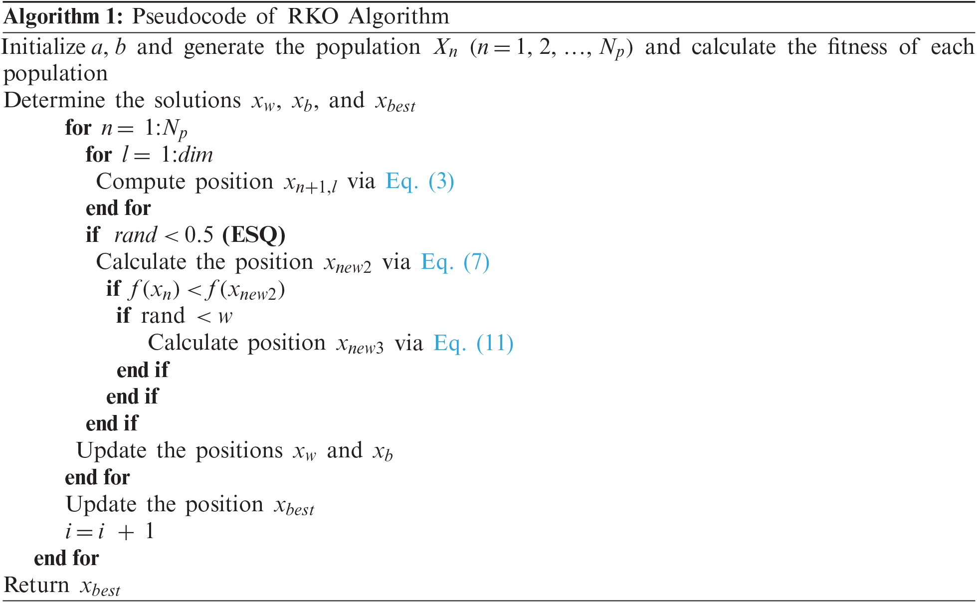
The authors of [3,6] presented an operator called the LEO, which is employed to boost the capabilities of a gradient-based optimizer. The LEO's updates ensure that the solutions are of superior quality. It can bypass local minima traps, and hence, it enhances convergence. LEO produces its
Else
End
End
where b is a normal distributed random number,
The
where
The value of
3.3 Development of Improved Runge-Kutta Optimization Algorithm
RKO algorithm struggles from being “trapped in the local minima situation.” Optimization could not be completed since the local region confined the system. This scenario often occurs in difficult and high-dimensional optimization problems. Additionally, producing new solutions is based on the results of the last iteration. This could slow down the algorithm's convergence speed, and hence, cause early convergence of the solutions. To increase search capabilities and handle difficult real-world problems, we enhance the RKO algorithm using the LEO concept. The proposed IRKO algorithm follows the RKO algorithm procedure step-by-step. LEO improves the diversification and intensification phase of the RKO algorithm along with the RK method. The initialization phase of the IRKO is similar to the RKO algorithm.
To examine the suggested solutions and improve the new suggested solutions in the next iteration, it is necessary to analyze the solutions in each iteration. As a result, each population is assessed to acquire its solution when each new population is randomly produced, an update that permits the new fitness to be upgraded using Eq. (3). Then, the new population is improved by the LEO mechanism, as mentioned in Eq. (12). Finally, the best position is achieved after updating the population using Eqs. (7) and (11) as similar to the RKO algorithm. Iterate the suggested IRKO until it meets the terminating condition. After that, the best option so far is discovered. The flowchart of the IRKO is shown in Fig. 1.
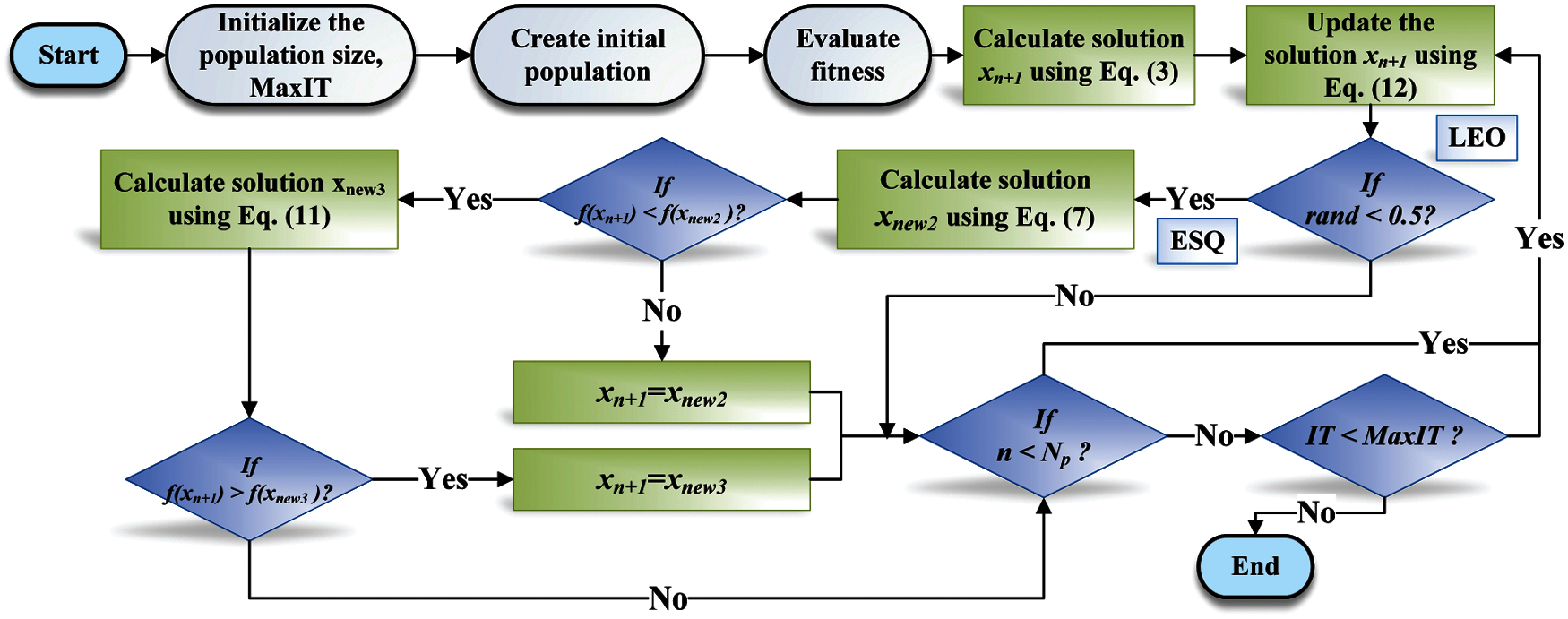
Figure 1: Flowchart of the IRKO algorithm
4 Numerical Simulation and Discussions
The performance of the IRKO is validated using twenty-three classical test benchmark functions and three real-world engineering problems. The IRKO has been simulated with a 30-population size and 500 maximum iterations to solve the benchmarks and engineering problems. The other control parameters are as follows. RKO and IRKO (a = 20 and b = 12), GWO and WOA (
Twenty-three benchmark functions, including unimodal, multi-modal, and fixed dimension multi-modal functions, were used to examine the IRKO's ability to exploit global solutions, explore the search space, and escape from the local minima trap. The benchmark test functions are provided in the weblink [39] for the reader's reference, in which the exploitation potential is assessed using the unimodal benchmarks (F1–F7), multi-modal benchmarks (F8–F13) meant to assess the exploration ability with a dimension of 30, and fixed dimension multi-modal test benchmarks (F14–F23) demonstrate the ability to explore low-dimensional search spaces. Several well-known optimization algorithms, such as GWO, HHO, SCA, IMO, HGSO, RKO, and WOA, have been evaluated against the same functions to confirm the superiority of the suggested IRKO algorithm. The simulation was carried out using a MATLAB 2020a installed on a laptop with an Intel Core i5 processor, 2.4 GHz clock speed, and 8 GB of RAM.
To confirm the performance of the proposed IRKO algorithm, the balance phase curve, average fitness curve, and trajectory curves are utilized and have been in Fig. 2. Fig. 2 shows the qualitative measures, such as the 2-D figure of all test functions (first column) and search history to confer the solutions in the search space (second column). The trajectory curves, balancing phase curves, and the average fitness curves are displayed in the third, fourth, and fifth columns of Fig. 2. In addition, Min, Mean, STD, and Run-Time (RT) values obtained by all selected algorithms are listed in Tab. 1. The boldface letters in the table indicate the best values. From Tab. 1, it is observed that the proposed IRKO produced the best results in terms of Min, Mean, and STD values on all 23 benchmark functions. However, the RT values of IRKO are slightly higher than the basic RKO version. This is due to the deployment of the LEO concept with the RKO algorithm. However, the proposed IRKO produces excellent performance in terms of reliability and robustness.
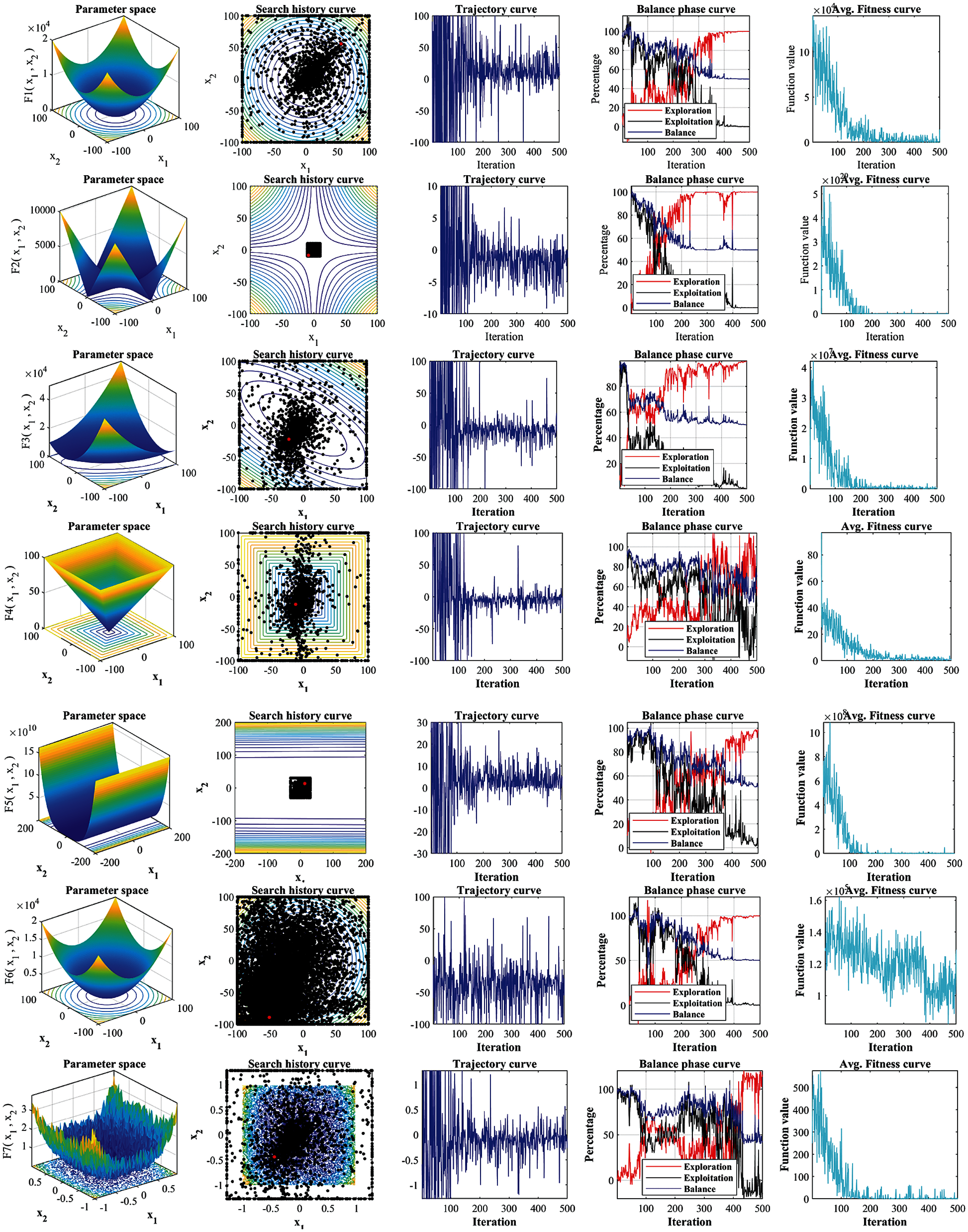
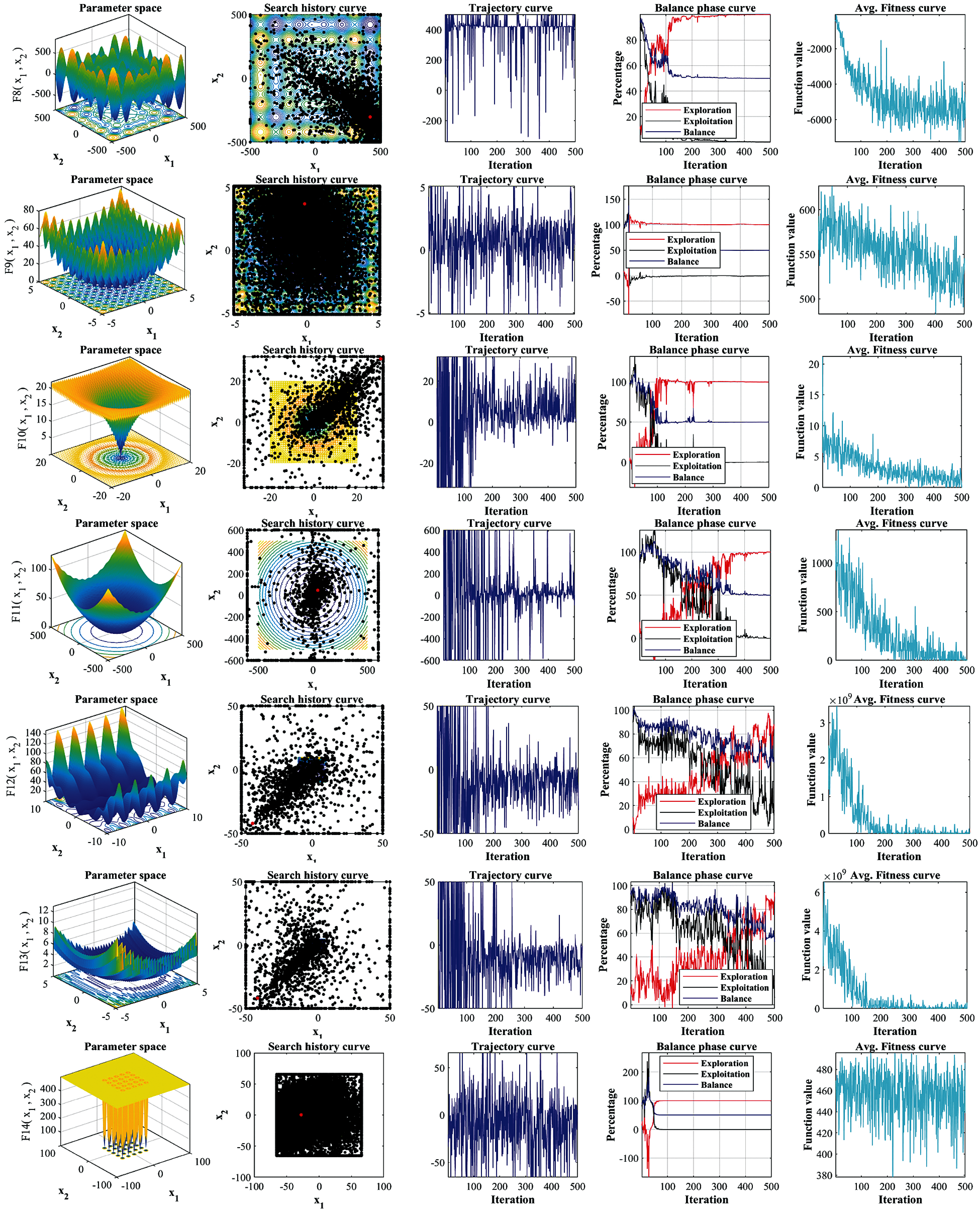

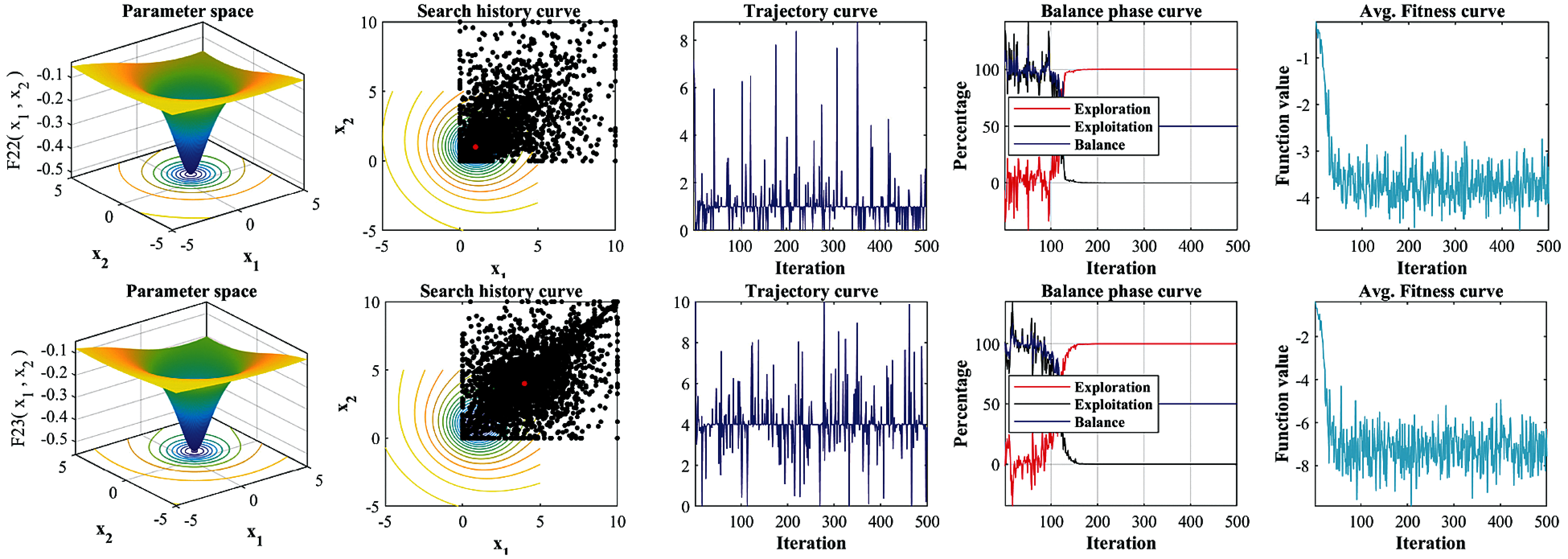
Figure 2: Qualitative results produced by IRKO algorithm on all selected benchmarks
The search's history explains how the algorithm search for the optimal solution in search space. The LEO concept enhances the behavior of the IRKO. This modality depicts the movement of the population about the best position for unimodal functions. The nature of the dispersion qualities of populations corresponds to the modality. When using IRKO to address multi-modal and unimodal functions, the exploration and exploitation capabilities are all enhanced. The trajectory curve indicated a high amplitude and frequency in the initial iterations and disappeared during the final iteration. As can be seen, IRKO has a high exploration ability early on and strong exploitation later on. Based on this behavior, the ideal approach is likely for the IRKO algorithm. The LEO in IRKO algorithm promotes the search optimization process to precisely and broadly focus on the local region. Compared to other recently proven methods, the LEO aids the RKO in efficiently and accurately discovering the search space. Fig. 3 illustrates the best solutions achieved so far throughout the iteration numbers. IRKO's convergence curves show a visible decay rate for unimodal functions. Meanwhile, other algorithms have a severe standstill, making the exploitation stage of the IRKO have a reliable exploration capability. The IRKO's multi-modal functions’ convergence curves indicate the seamless transition between exploitation and exploration.
It converges quickly with better results than the other counterparts in most of the remaining test functions. This is evident when it's understood that the IRKO performs well between exploitation and exploration stages since it captures nearby values for the best solutions. These solutions are exploited proficiently throughout the iterations to offer the best solutions. In addition, the reliability of all selected algorithms is assessed by visualizing the boxplot. Fig. 4 shows the boxplot analysis of all algorithms on selected benchmarks. It is visualized that the reliability of the proposed IRKO is superior to all other selected algorithms. To rank all algorithms, Friedman's rank test is carried out, and the FRT values of all algorithms are listed in Tab. 2. It is observed from Tab. 2 that the proposed IRKO algorithm stands first in most of the benchmark functions.
4.2 Real-World Optimization Problems
In this subsection, the IRKO algorithm has been tested in addressing three real-world engineering design problems, including welded beam, tension/compression spring, and pressure vessel. All these design problems have many inequality constraints. The method gets substantial solutions if it violates any of the criteria using the death penalty function.

The primary objective of the problem depicted in Fig. 5 is to minimize the cost of the welded beam and find the best cost by considering the constraints. The design variables are length (l), the thickness of the bar (b), the thickness of the weld (h), and height (t). It has constraints, such as beam end deflection (δ), bar buckling load (Pc), shear stress (τ), beam blending stress (θ), and side constraints, and consider x = [x1, x2, x3, x4] = [h, l, t, b]. The variable ranges are
Subjected to constraints:
Tab. 3 lists the results obtained by the IRKO and other selected algorithms, including RKO, GWO, HHO, WOA, IMO, HGSO, and SCA. From Tab. 3, it can be seen that the IRKO performing better than all selected methods and attained the minimum cost. Tab. 3 also lists the statistical data, such as Min, Mean, STD, and RT. Therefore, it is determined that the reliability of the suggested IRKO algorithm is better for the engineering design problem. Fig. 6 depicts the convergence curves and box plots of all algorithms while handling the problem. In addition, FRT values obtained by all algorithms are also listed. The proposed IRKO algorithm stands first in solving the welded beam design problem also.
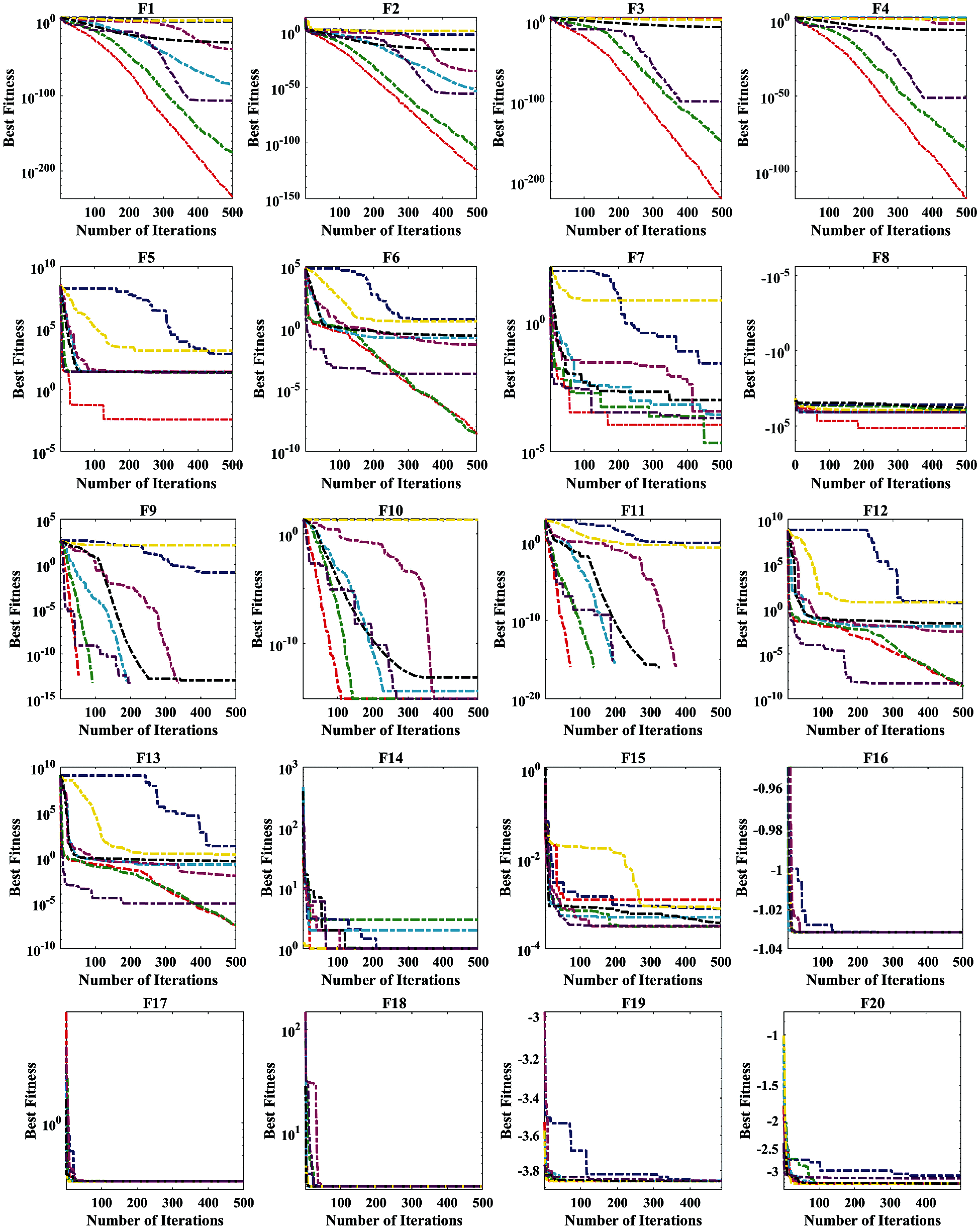
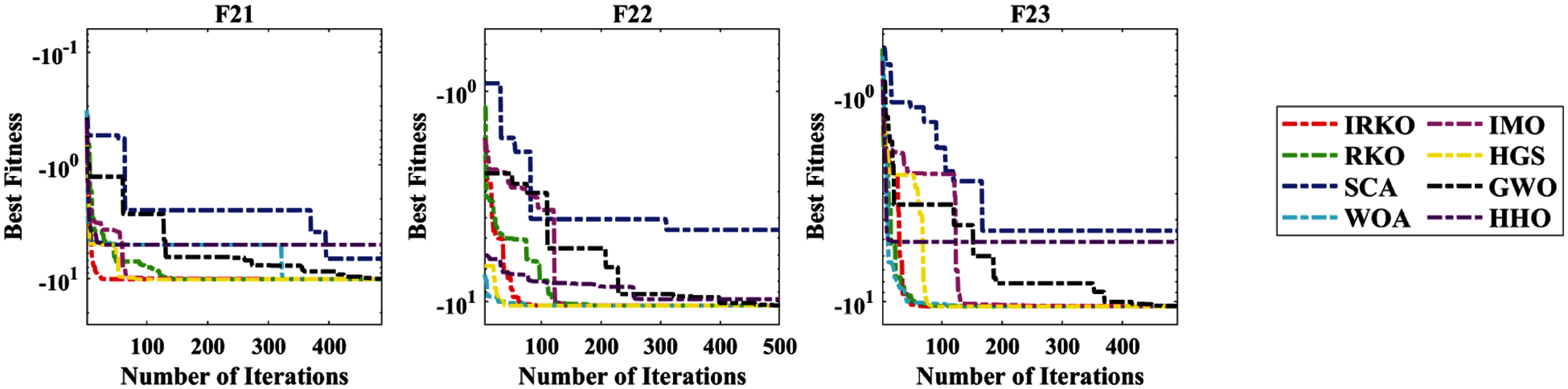
Figure 3: Convergence performance of all selected algorithms on traditional benchmarks
4.2.2 Tension/Compression Spring Design
Compression spring design has been considered as yet alternative traditional mechanical engineering problem. This problem is illustrated in Fig. 7, and the primary objective of this problem is to minimize the tension spring weight of the framework. The design variables of the tension/compression spring design problem are active coils (N), wire diameter (d), and mean coil diameter (D), and consider x = [x1, x2, x3] = [d, D, N]. The variable ranges are
Subjected to constraints:
Tab. 4 lists the results obtained by the IRKO and other selected algorithms, including RKO, GWO, HHO, WOA, IMO, HGSO, and SCA. From Tab. 4, it can be seen that the IRKO performing better than all other selected algorithms and attained the minimum tension spring weight. Tab. 4 also lists the statistical data, such as Min, Mean, STD, and RT. Therefore, it is determined that the reliability of the suggested IRKO algorithm is better for the compression spring design problem. Fig. 8 depicts the convergence curves and box plots of all algorithms while handling the problem. In addition, FRT values obtained by all algorithms are also listed. The proposed IRKO algorithm stands first in solving the tension/compression spring design problem also.
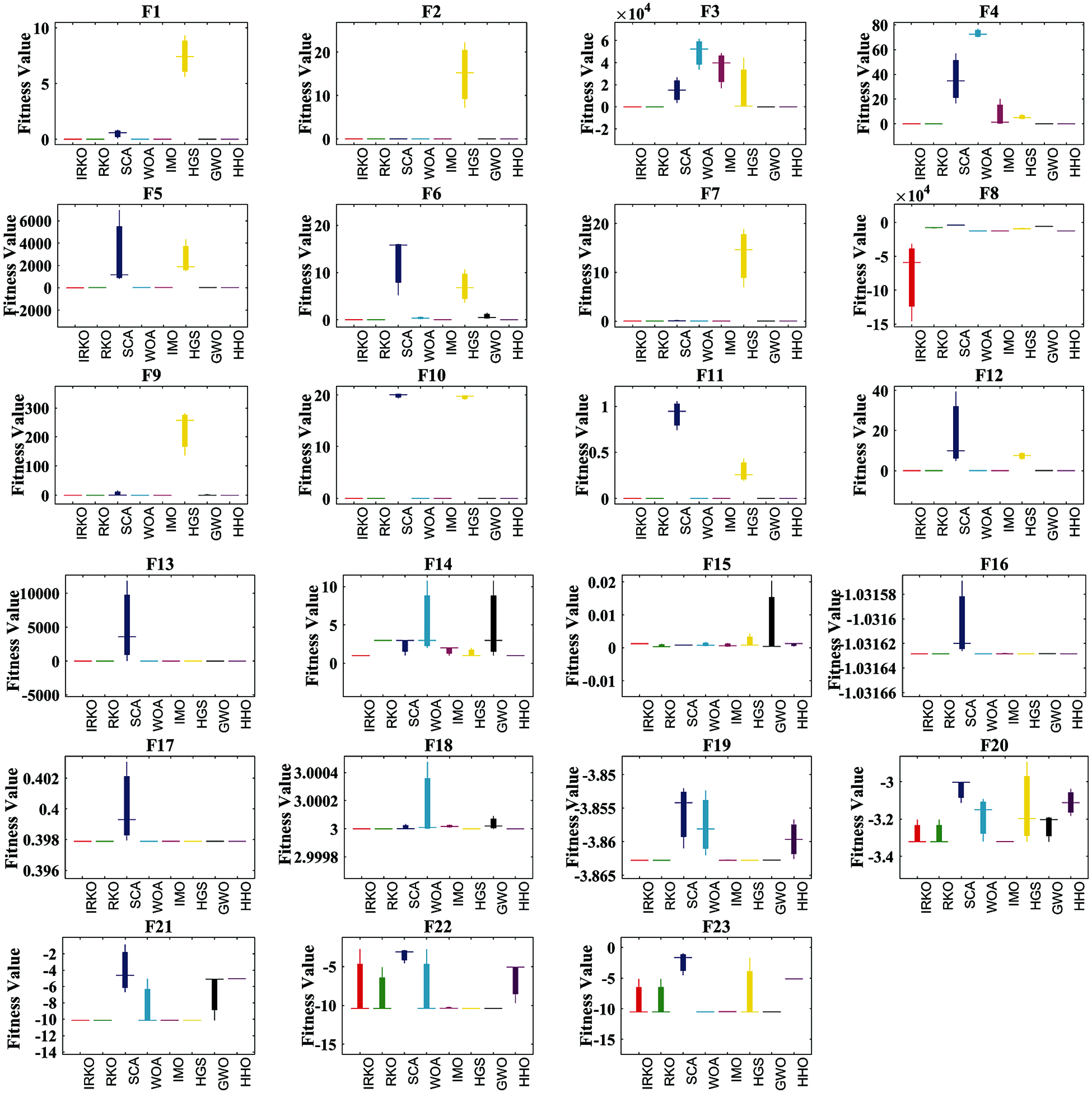
Figure 4: Boxplot analysis of all algorithms on selected benchmark functions
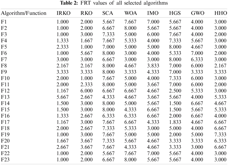
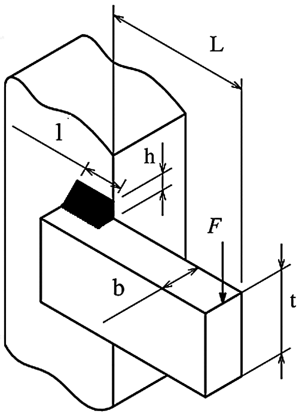
Figure 5: Welded beam design optimization problem

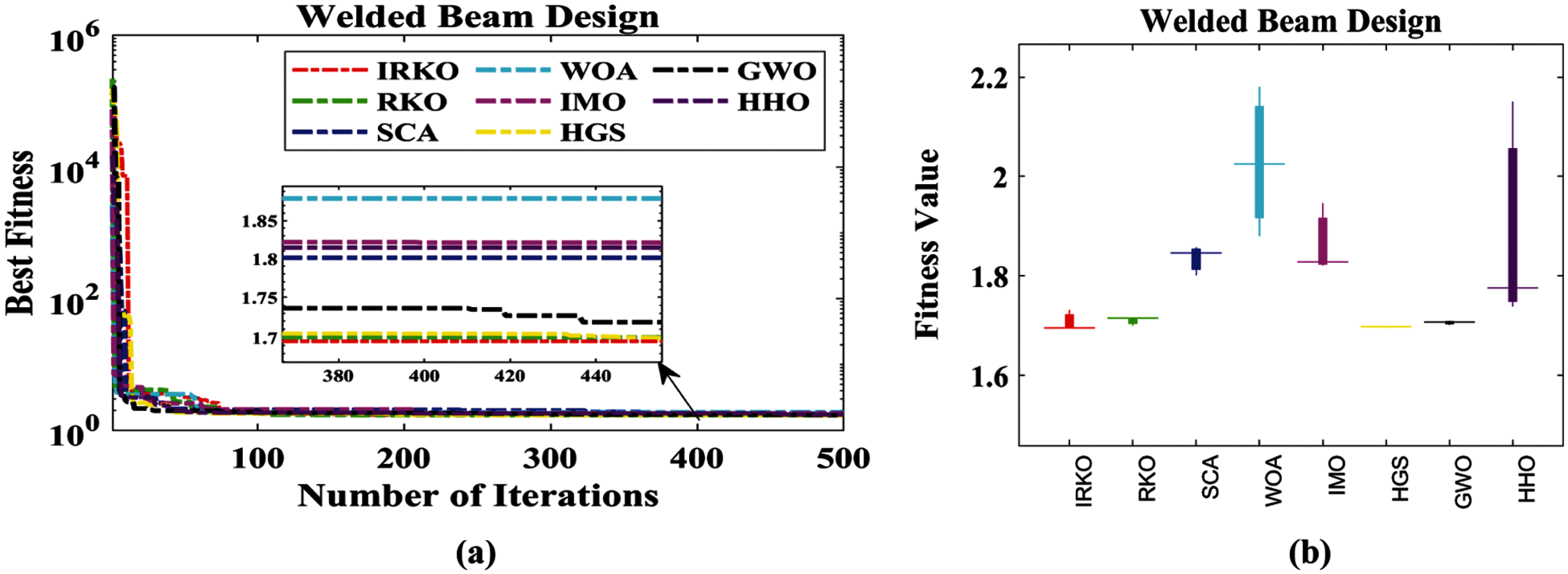
Figure 6: Curves of all algorithms for the welded beam design; (a) Convergence curve, (b) Boxplot
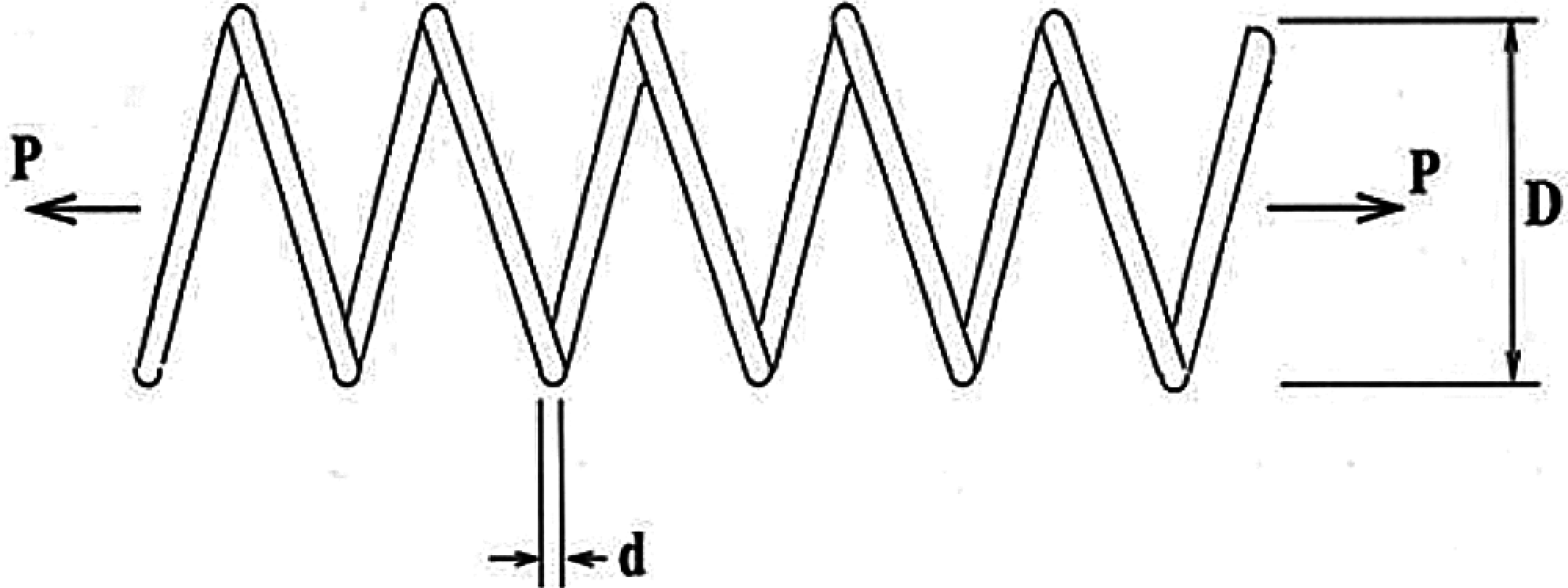
Figure 7: Tension/Compression spring design problem
The graphic view of the pressure vessel design framework is shown in Fig. 9. The pressure vessel has hemispherical heads and capped ends. The key objective is to minimize the construction cost. It has four constraints and four parameters (i.e., the length of the cylindrical section (L), the thickness of the head (Th), the inner radius (R), and the thickness of the shell (Ts)), and consider x = [x1x2x3x4] = [TsThRL]. The variable ranges are
Subjected to constraints:
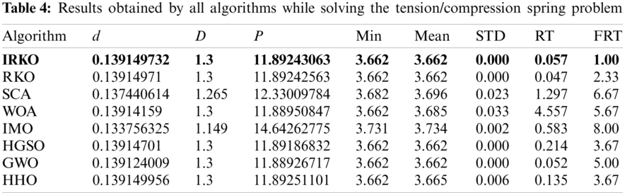
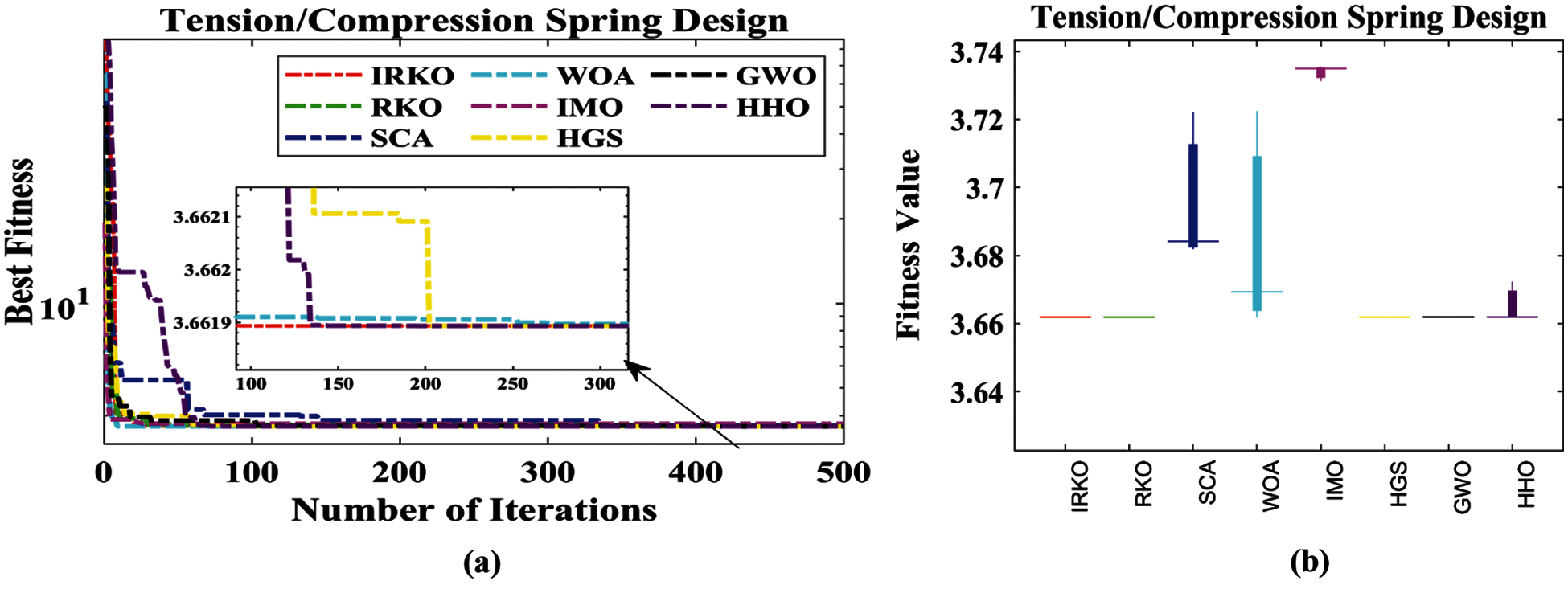
Figure 8: Curves of all algorithms for the compression spring; (a) Convergence curve, (b) Boxplot
Tab. 5 lists the results found by the IRKO and several selected algorithms, including RKO, GWO, HHO, WOA, IMO, HGSO, and SCA. From Tab. 5, it can be seen that the IRKO performing better than all other selected algorithms and attained the minimum construction cost. Tab. 5 also lists the statistical data, such as Min, Mean, STD, and RT. Therefore, it is concluded that the reliability of the proposed IRKO algorithm is better for the pressure vessel design problem. Fig. 10 depicts the convergence curves and box plots of all algorithms while handling the problem. In addition, FRT values obtained by all algorithms are also listed. The proposed IRKO algorithm stands first in solving the pressure vessel design problem.
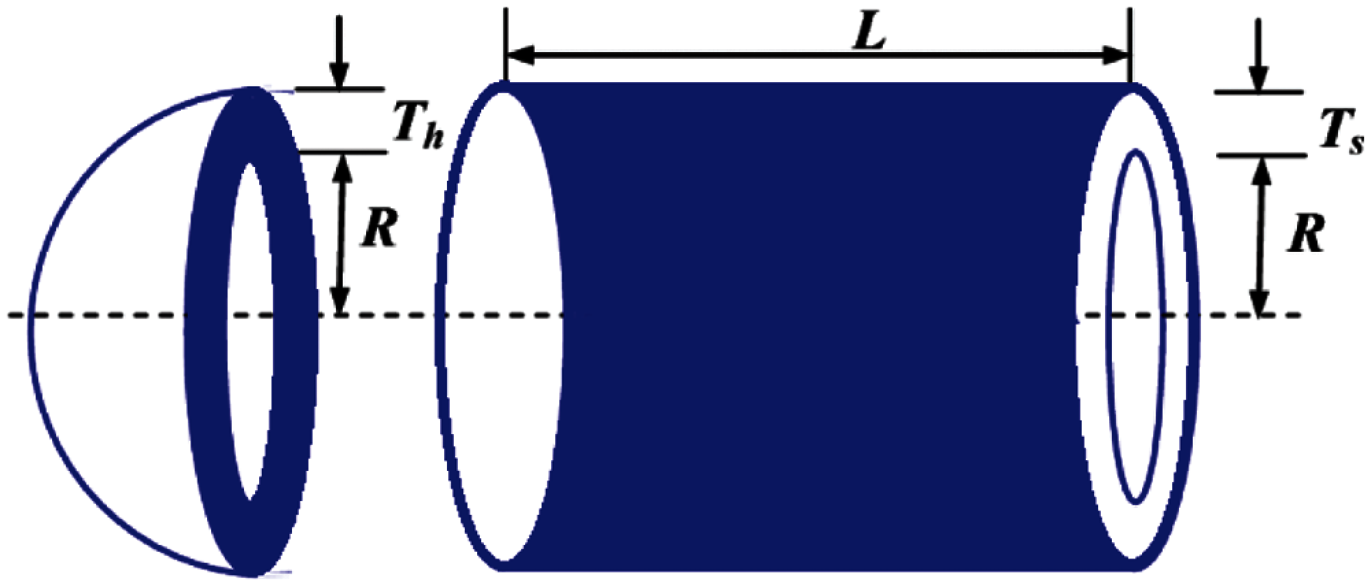
Figure 9: Pressure vessel design problem
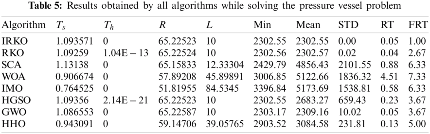
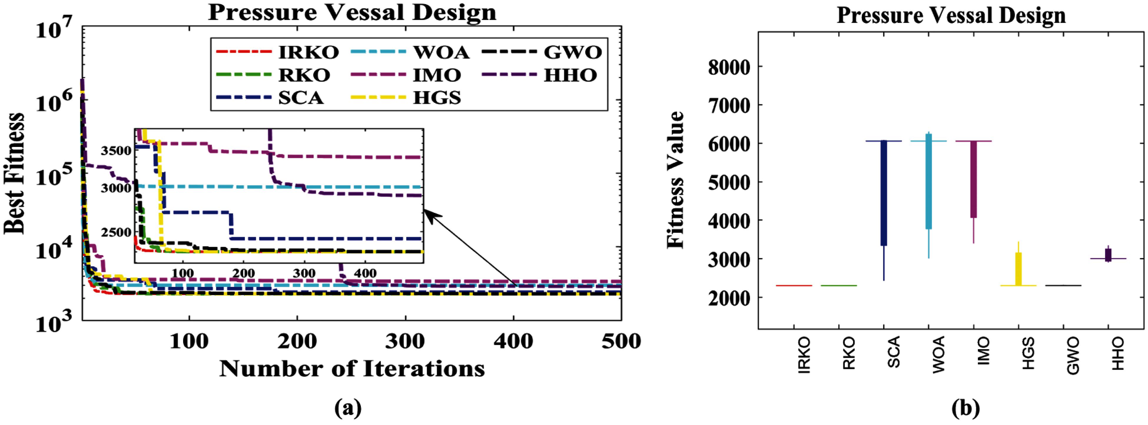
Figure 10: Curves of all algorithms for the pressure vessel problem; (a) Convergence curve, (b) Boxplot
In this paper, an enhanced variant of the RKO algorithm called IRKO algorithm is proposed. A local escaping operator concept is employed to improve the characteristics, i.e., exploration and exploitation capabilities of the original RKO algorithm. A 23 classical test suite and three engineering design problems—welded beam, tension/compression spring, and pressure vessel design problems are used to assess the performance of the IRKO algorithm. According to benchmark tests’ statistical findings, the IRKO produced outcomes that were either superior or relatively close to other selected algorithms. Furthermore, it may assess the proposed IRKO's suitability to real-world applications based on actual investigations of design problems.
From the earlier analysis, the IRKO might enable a broad range of future tasks. This includes applying the IRKO algorithm in numerous applications, such as image processing, feature selection, PV parameter estimation, power systems, power electronics, smart grid, big data applications, data mining applications, signal denoising, wireless sensor networks, artificial intelligence, machine learning, and other benchmark functions. Also applicable to situations depending on binary-, multi-, and many-objective optimizations.
Acknowledgement: The authors extend their appreciation to the Deanship of Scientific Research at King Khalid University, Saudi Arabia, for funding this work through the Research Group Program under Grant No: RGP. 2/108/42.
Funding Statement: The authors received no specific funding for this study.
Conflicts of Interest: The authors declare that they have no conflicts of interest to report regarding the present study.
1. J. D. Schaffer, Some Experiments in Machine Learning Using Vector Evaluated Genetic Algorithms. Nashville, USA: Vanderbilt University, pp. 115–152, 1985. [Google Scholar]
2. W. K. Wong and C. I. Ming, “A review on metaheuristic algorithms: Trends, benchmarking and applications,” in Proc. of Int. Conf. on Smart Computing and Communications, Malaysia, pp. 1–5, 2019. [Google Scholar]
3. M. Premkumar, P. Jangir and R. Sowmya, “MOGBO: A new multiobjective gradient-based optimizer for real-world structural optimization problems,” Knowledge-Based Systems, vol. 218, pp. 106856, 2021. [Google Scholar]
4. M. Premkumar, R. Sowmya, J. Pradeep, K. S. Nisar and M. Aldhaifallah, “A new metaheuristic optimization algorithms for brushless direct current wheel motor design problem,” Computers, Materials & Continua, vol. 67, no. 2, pp. 2227–2242, 2021. [Google Scholar]
5. M. Premkumar, P. Jangir, B. Santhosh Kumar, R. Sowmya, H. H. Alhelou et al., “A new arithmetic optimization algorithm for solving real-world multiobjective CEC-2021 constrained optimization problems: Diversity analysis and validations,” IEEE Access, vol. 9, pp. 84263–84295, 2021. [Google Scholar]
6. I. Ahmadianfar, O. Bozorg-haddad and X. Chu, “Gradient-based optimizer: A new metaheuristic optimization algorithm,” Information Sciences, vol. 540, pp. 131–159, 2020. [Google Scholar]
7. S. Kumar, P. Jangir, G. G. Tejani, M. Premkumar and H. H. Alhelou, “MOPGO: A new physics-based multi-objective plasma generation optimizer for solving structural optimization problems,” IEEE Access, vol. 9, pp. 84982–85016, 2021. [Google Scholar]
8. B. A. Khateeb, K. Ahmed, M. Mahmod and D. N. Le, “Rock hyraxes swarm optimization: A new nature-inspired metaheuristic optimization algorithm,” Computers, Materials & Continua, vol. 68, no. 1, pp. 643–654, 2021. [Google Scholar]
9. R. Fessi1, H. Y. Rezk and S. Bouallègue, “Grey wolf optimization-based tuning of terminal sliding mode controllers for a quadrotor,” Computers, Materials & Continua, vol. 68, no. 2, pp. 2265–2282, 2021. [Google Scholar]
10. D. H. Wolpert and W. G. Macready, “No free lunch theorems for optimization,” IEEE Transactions on Evolutionary Computation, vol. 1, no. 1, pp. 67–82, 1997. [Google Scholar]
11. A. Iman, A. H. Ali, A. H. Gandomi, X. Chu and H. Chen, “RUN beyond the metaphor: An efficient optimization algorithm based on runge kutta method,” Expert Systems with Applications, vol. 181, pp. 115079, 2021. [Google Scholar]
12. M. Premkumar, P. Jangir, C. Ramakrishnan, G. Nalinipriya, H. H. Alhelou et al., “identification of solar photovoltaic model parameters using an improved gradient-based optimization algorithm with chaotic drifts,” IEEE Access, vol. 9, pp. 62347–62379, 2021. [Google Scholar]
13. R. Eberhart and J. Kennedy, “A new optimizer using particle swarm theory,” in Proc. of the Sixth Int. Symp. on Micro Machine and Human Science, Japan, pp. 39–43, 1995. [Google Scholar]
14. M. Dorigo, V. Maniezzo and A. Colorni, “Ant system: Optimization by a colony of cooperating agents,” IEEE Transactions on Systems, Man, and Cybernetics: Part B (Cybernetics), vol. 26, no. 1, pp. 29–41, 1996. [Google Scholar]
15. W. C. Wang, L. Xu, K. W. Chau and D. M. Xu, “Yin-yang firefly algorithm based on dimensionally Cauchy mutation,” Expert Systems with Applications, vol. 150, pp. 113216, 2020. [Google Scholar]
16. D. Oliva, E. Cuevas and G. Pajares, “Parameter identification of solar cells using artificial bee colony optimization,” Energy, vol. 72, pp. 93–102, 2014. [Google Scholar]
17. S. Mirjalili, S. M. Mirjalili and A. Lewis, “Grey wolf optimizer,” Advances in Engineering Software, vol. 69, pp. 46–61, 2014. [Google Scholar]
18. A. A. Heidari, S. Mirjalili, H. Faris, I. Aljarah, M. Mafarja et al., “Harris hawks optimization: Algorithm and applications,” Future Generation Computer Systems, vol. 97, pp. 849–872, 2019. [Google Scholar]
19. N. Rana, M. S. A. Latiff, S. M. Abdulhamid and H. Chiroma, “Whale optimization algorithm: A systematic review of contemporary applications,” Neural Computing and Applications, vol. 32, pp. 16245–16277, 2020. [Google Scholar]
20. L. Abualigah, D. Yousri, M. Abd Elaziz, A. A. Ewees, M. A. A. Al-Qaness et al., “Aquila optimizer: A novel meta-heuristic optimization algorithm,” Computers & Industrial Engineering, vol. 157, pp. 107250, 2021. [Google Scholar]
21. M. Premkumar, R. Sowmya, P. Jangir, H. H. Alhelou, A. A. Heidari et al., “MOSMA: Multi-objective slime mould algorithm based on elitist non-dominated sorting,” IEEE Access, vol. 9, pp. 3229–3248, 2021. [Google Scholar]
22. A. Faramarzi, M. Heidarinejad, S. Mirjalili and A. H. Gandomi, “Marine predators algorithm: A nature-inspired metaheuristic,” Expert Systems with Applications, vol. 152, pp. 113377, 2020. [Google Scholar]
23. A. Faramarzi, M. Heidarinejad, B. Stephens and S. Mirjalili, “Equilibrium optimizer: A novel optimization algorithm,” Knowledge-Based Systems, vol. 191, pp. 105190, 2020. [Google Scholar]
24. M. Premkumar, C. Kumar, R. Sowmya and J. Pradeep, “A novel salp swarm assisted hybrid maximum power point tracking algorithm for the solar PV power generation systems,” Automatika, vol. 62, no. 1, pp. 1–20, 2021. [Google Scholar]
25. D. E. Goldberg and J. H. Holland, “Genetic algorithms and machine learning,” Machine Learning, vol. 3, no. 2, pp. 95–99, 1988. [Google Scholar]
26. F. Huang, L. Wang and Q. He, “An effective co-evolutionary differential evolution for constrained optimization,” Applied Mathematics and Computation, vol. 186, no. 1, pp. 340–356, 2007. [Google Scholar]
27. Q. Niu, L. Zhang and K. Li, “A biogeography-based optimization algorithm with mutation strategies for model parameter estimation of solar and fuel cells,” Energy Conversion and Management, vol. 86, pp. 1173–1185, 2014. [Google Scholar]
28. M. H. Qais, H. M. Hasanien and S. Alghuwainem, “identification of parameters for three-diode photovoltaic model using analytical and sunflower optimization algorithm,” Applied Energy, vol. 250, pp. 109–117, 2019. [Google Scholar]
29. D. Tang, S. Dong, Y. Jiang, H. Li and Y. Huang, “ITGO: Invasive tumor growth optimization algorithm,” Applied Soft Computing, vol. 36, pp. 670–698, 2015. [Google Scholar]
30. R. V. Rao, V. J. Savsani and J. Balic, “Teaching-learning-based optimization algorithm for unconstrained and constrained optimization problems,” Engineering Optimization, vol. 44, no. 12, pp. 1447–1462, 2012. [Google Scholar]
31. Y. Yang, H. Chen, A. A. Heidari and A. H. Gandomi, “Hunger games search: Visions, conception, implementation, deep analysis, perspectives, and towards performance shifts,” Expert Systems with Applications, vol. 177, pp. 114864, 2021. [Google Scholar]
32. M. Premkumar, R. Sowmya, P. Jangir and J. S. V. Siva Kumar, “A new and reliable objective functions for extracting the unknown parameters of solar photovoltaic cell using political optimizer algorithm,” in Proc. of Int. Conf. on Data Analytics for Business and Industry, Bahrain, pp. 1–6, 2020. [Google Scholar]
33. A. Banerjee, V. Mukherjee and S. P. Ghoshal, “An opposition-based harmony search algorithm for engineering optimization problems,” Ain Shams Engineering Journal, vol. 5, no. 1, pp. 85–101, 2014. [Google Scholar]
34. M. Premkumar, P. Jangir, R. Sowmya, R. M. Elavarasan and B. S. Kumar, “Enhanced chaotic JAYA algorithm for parameter estimation of photovoltaic cell/modules,” ISA Transactions, Article in press, pp. 1–28, 2021. [Google Scholar]
35. M. Premkumar, T. S. Babu, S. Umashankar and R. Sowmya, “A new metaphor-less algorithms for the photovoltaic cell parameter estimation,” Optik, vol. 208, pp. 164559, 2020. [Google Scholar]
36. E. Rashedi, H. N. Pour and S. Saryazdi, “GSA: A gravitational search algorithm,” Information Sciences, vol. 179, no. 13, pp. 2232–2248, 2009. [Google Scholar]
37. S. Mirjalili, “SCA: A sine cosine algorithm for solving optimization problems,” Knowledge-Based Systems, vol. 96, pp. 120–133, 2016. [Google Scholar]
38. B. Javidy, A. Hatamlou and S. Mirjalili, “Ions motion algorithm for solving optimization problems,” Applied Soft Computing, vol. 32, pp. 72–79, 2015. [Google Scholar]
39. M. Premkumar, “Classical benchmark test functions,” 2021. [Online]. Available: https://premkumarmanoharan.wixsite.com/mysite/downloads [Accessed: April 25, 2021]. [Google Scholar]
 | This work is licensed under a Creative Commons Attribution 4.0 International License, which permits unrestricted use, distribution, and reproduction in any medium, provided the original work is properly cited. |