DOI:10.32604/cmc.2022.020886
| Computers, Materials & Continua DOI:10.32604/cmc.2022.020886 | |
| Article |
Automatic Detection of Nephrops Norvegicus Burrows from Underwater Imagery Using Deep Learning
1ETSI Telecomunicación, Universidad de Málaga, Málaga, 29071, Spain
2Department of Computer Science, National University of Technology, Islamabad, 44000, Pakistan
3Instituto Español de Oceanografía, Centro Oceanográfico de Cádiz, Cádiz, 39004, Spain
4Marine Institute Rinville, Oranmore, Ireland
*Corresponding Author: Atif Naseer. Email: atif@uma.es
Received: 12 June 2021; Accepted: 12 August 2021
Abstract: The Norway lobster, Nephrops norvegicus, is one of the main commercial crustacean fisheries in Europe. The abundance of Nephrops norvegicus stocks is assessed based on identifying and counting the burrows where they live from underwater videos collected by camera systems mounted on sledges. The Spanish Oceanographic Institute (IEO) and Marine Institute Ireland (MI-Ireland) conducts annual underwater television surveys (UWTV) to estimate the total abundance of Nephrops within the specified area, with a coefficient of variation (CV) or relative standard error of less than 20%. Currently, the identification and counting of the Nephrops burrows are carried out manually by the marine experts. This is quite a time-consuming job. As a solution, we propose an automated system based on deep neural networks that automatically detects and counts the Nephrops burrows in video footage with high precision. The proposed system introduces a deep-learning-based automated way to identify and classify the Nephrops burrows. This research work uses the current state-of-the-art Faster RCNN models Inceptionv2 and MobileNetv2 for object detection and classification. We conduct experiments on two data sets, namely, the Smalls Nephrops survey (FU 22) and Cadiz Nephrops survey (FU 30), collected by Marine Institute Ireland and Spanish Oceanographic Institute, respectively. From the results, we observe that the Inception model achieved a higher precision and recall rate than the MobileNet model. The best mean Average Precision (mAP) recorded by the Inception model is 81.61% compared to MobileNet, which achieves the best mAP of 75.12%.
Keywords: Faster RCNN; computer vision; nephrops norvegicus; nephrops norvegicus stock assessment; underwater videos classification
The earth's ecosystem is mainly composed of oceans, as it produces 50% of the oxygen and 97% of the water. Also, it is a significant source of our daily food as it provides 15% of proteins in the form of marine animals. There are many studies in terrestrial ecosystems than in marine ecosystems because it is more challenging to study the marine ecosystem, especially in the deeper areas. Monitoring the habitats of marine species is a challenging task for biologists and marine experts. The environment features such as depth-based color variations and the turbidity or movement of species make it a challenge [1]. Several years ago, marine scientists used satellite, shipborne sensors, and camera sensors to collect underwater species’ images. In recent years with the advancement of technology, scientists use underwater Remotely Operated Vehicles (ROVs), Autonomous Underwater Vehicles (AUVs), sledge and drop frame structures equipped with high-definition cameras to record the videos and images of marine species. These vehicles can capture high-definition images and videos. Besides all this quality equipment, the underwater environment is still a challenge for scientists and marine biologists. The two main factors which make it difficult are the free natural environment and variations of the visual content, which may arise from variable illumination, scales, views, and non-rigid deformations [2].
The Norway lobster, Nephrops norvegicus, is one of the main commercial crustacean fisheries in Europe, where in 2018, the total allowable catch (TAC) was set at 32,705 tons for International Council for the Exploration of the Sea (ICES) areas 7, 8 and 9 [3]. Fig. 1 shows an individual Nephrops specimen. This species can be found in sandy-muddy sediments from 90 m to 800 m depth in the Atlantic NE waters and the Mediterranean Sea [4], where the sediment is suitable for constructing their burrows. Nephrops spend most of the time inside the burrows, and their emergence behavior is influenced by several factors: time of year, light intensity, tidal strength. These burrows can be detected through optimal lighting set-up during video recordings of the seabed. The burrows themselves can be easily identified from surface features once specialist training has been taken [5].
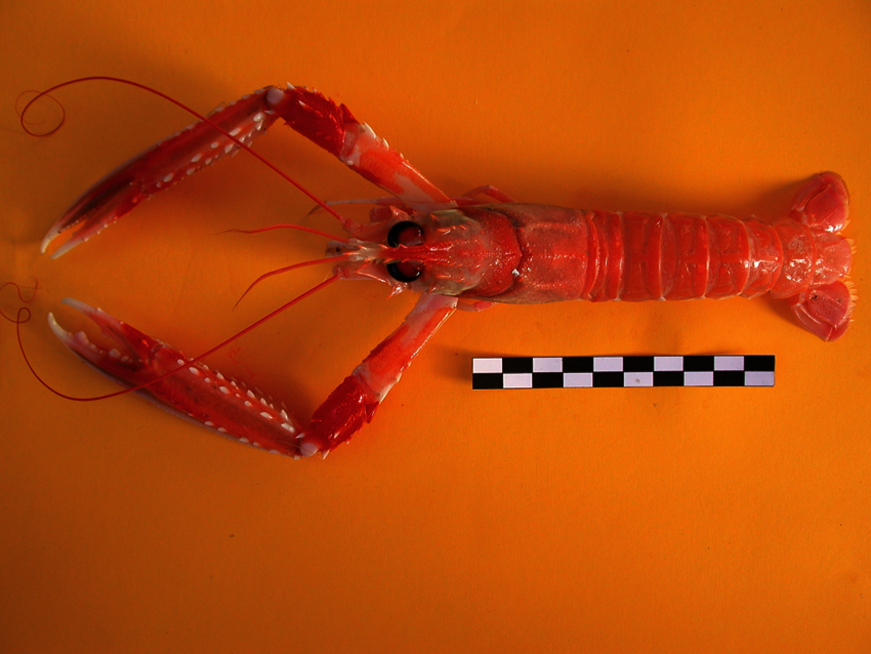
Figure 1: Nephrops norvegicus
A Nephrops burrow system typically can have single to multiple openings to different tunnels. A unique individual is assumed to occupy a burrow system [6]. Burrows show signature features that are specific to Nephrops, as shown in Fig. 2. They can be summarized as follows:
1. At least one burrow opening is particularly half-moon shape.
2. There is often proof of expelled sediment, typically in a wide delta-like ‘fan’ at the tunnel opening, and scratches and tracks are frequently evident.
3. The centre of all the burrow openings has a raised structure.
4. Nephrops may be present (either in or out of burrow).
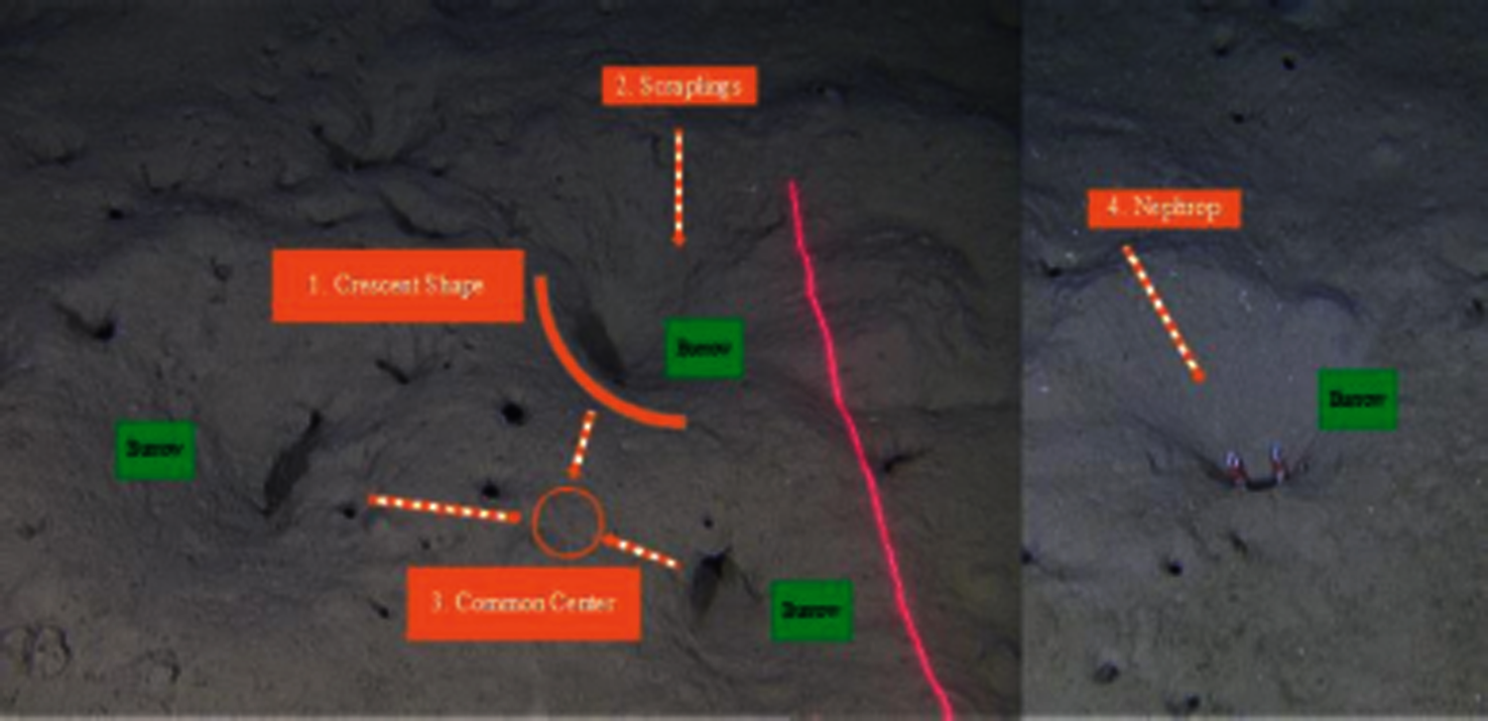
Figure 2: Nephrops burrows signature features
The Nephrops burrow system composed of one or more than one burrows of above-mentioned characteristics. The presence of more than one burrow nearby doesn't means the presence of more than one Nephrops.
The ICES is an international organization of 20 member countries. ICES is working on the marine sciences with more than 6000 scientists from 7000 different marine institutes of the member countries [7]. The working group on Nephrops Surveys (WGNEPS) is the expert group that specializes in Nephrops norvegicus underwater television and trawl surveys within ICES [6–8].
UWTV surveys to monitor the abundance of Nephrops populations were pioneered in Scotland in the early 90's. The estimation of Norway lobster populations using this method involves identifying and quantifying burrow density over the known area of Nephrops distribution that can be used as an abundance index of the stock [5,9]. Nephrops abundance from UWTV surveys is the basis of assessment and advice for managing these stocks [9].
Nephrops populations are assessed and managed by Functional Units (FU) where there is a specific survey for each FU. In 2019, a total of 19 surveys had conducted that cover the 25 FU's in ICES and one geographical subarea (GSA) in the Adriatic Sea [10] and shown in Fig 3. These surveys were conducted using standardized equipment and agreed protocols under the remit of WGNEPS.
This study considers data from the Gulf of Cadiz (FU 30) and the Smalls (FU 22) Nephrops grounds to detect the Nephrops’ burrows using the image data collected from different stations in each FU using our proposed methodology.
The underwater environment is hard to analyse as it presents formidable challenges for Computer Vision and machine learning technologies. The image classification and detection in underwater images are quite different as compared to other visual data. Also, data collection in an underwater environment is the biggest challenge. One reason for this is light, as light and water are not considered good friends because when light passes through the water, it cannot absorb and reach the sea surface, which makes the images or videos a blurring effect. Also, scattering, and non-uniform lighting make the environment more challenging for data collection.
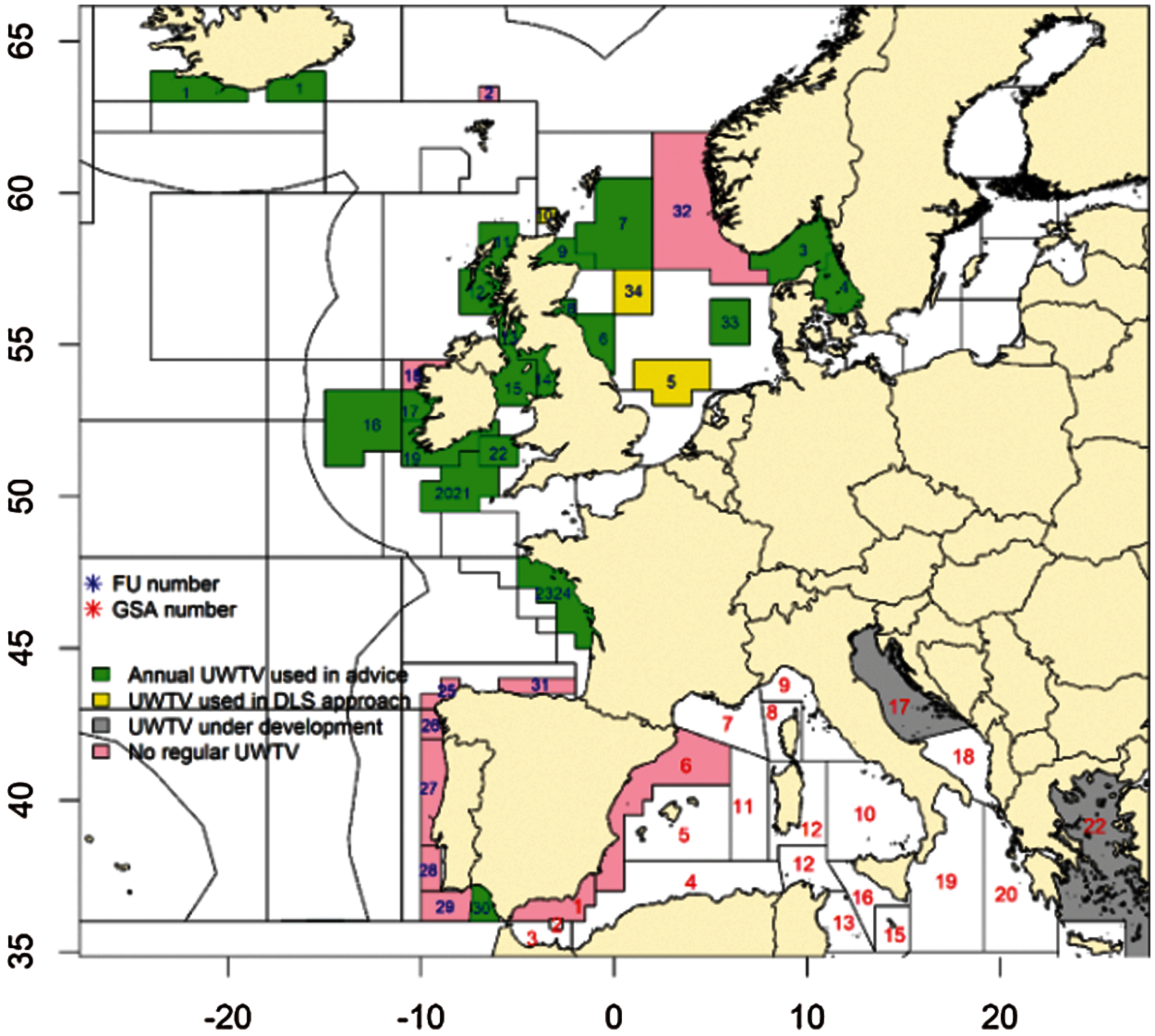
Figure 3: Nephrops UWTV survey coverage in 2019 (FU: Functional unit, GSA: Geographical sub area, DLS: data limited stock). the gulf of cadiz nephrops ground (FU 30) and the smalls nephrops ground (FU 22) [10]
Poor visibility is a common problem in the underwater environment. The poor visibility is due to the ebb and flow of tides and that cause fine mud particles to suspend in the water column. The ocean current is another factor that causes frequent luminosity change. The visual features like lightning conditions, colour changes, turbidity, and low pixel resolution make it challenging. Some of the environmental features such as depth-based colour variations and the turbidity or movement of species make the data collection very difficult in an underwater environment [1]. Thus, two main factors which make it difficult are the free natural environment and variations of the visual content, which may arise from variable illumination, scales, views, and non-rigid deformations [2].
Nephrops data are collected, and UWTV surveys are reviewed manually by trained experts. Many of the data were difficult to process due to complex environmental conditions. Burrows systems are quantified following the protocol established by ICES [6,8]. The image data (where this refers to video or stills data) for each station is reviewed independently by at least two experts, and the counts are recorded for each minute onto log sheet records. Each row of the log sheet records the minute, the number of burrows system count, and the time stamp. Count data are screened to check for any unusual discrepancies using Lin's Concordance Correlation Coefficient (CCC) with a threshold of 0.5. Lin's CCC [11] measures the ability of counters to precisely reproduce each other's counts on a scale of 0.5 to 1, where 1 is perfect concordance. Only stations with a threshold lower than 0.5 were reviewed again by the experts. Fig. 4 shows the current methodology used for the counting of Nephrops burrows.
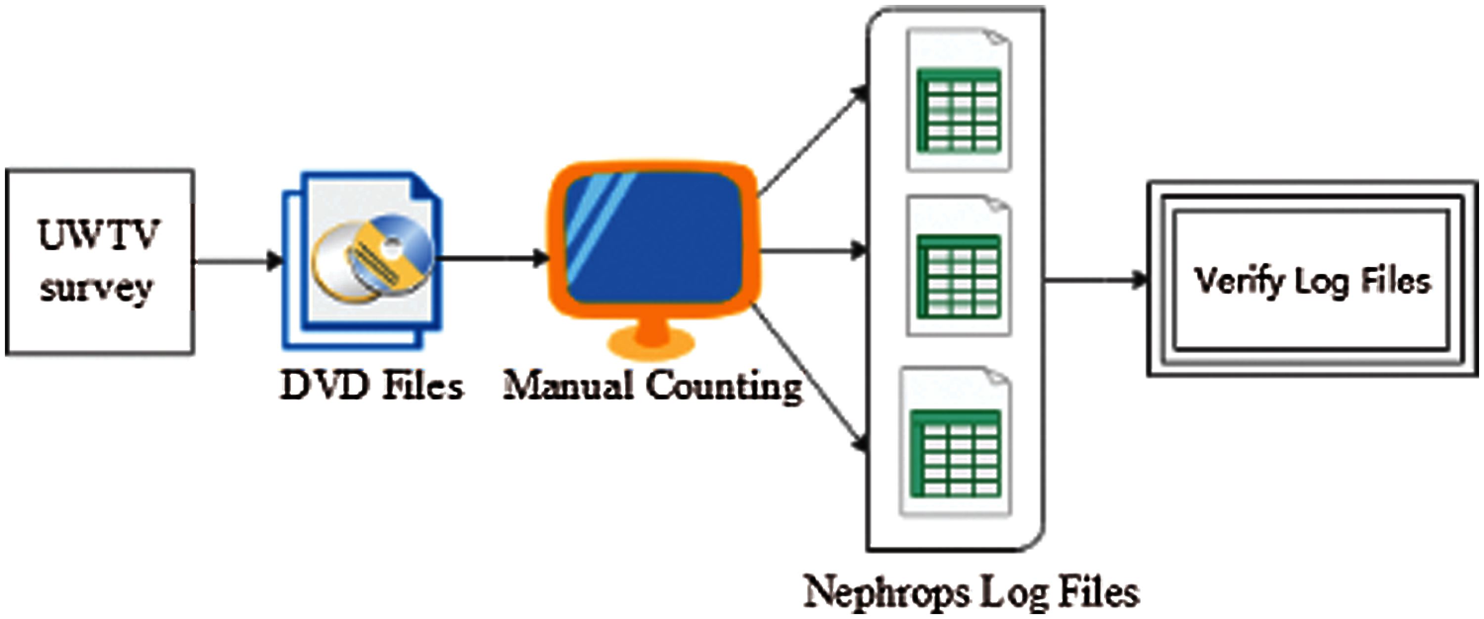
Figure 4: Current methodology for nephrops norvegicus burrows count
With the massive amount of data collected for videos and images, manually annotating and analysing it is a laborious job and requires a lot of data review and processing time. Due to limited human capabilities, the manual review of image data requires a lot of time by trained experts to process the data to be quality controlled and ready for use in stock assessment. Due to these factors, only a limited amount of collected data is used for analysis that usually does not provide deep insights into a problem [12].
Many scientists employ Artificial Intelligence-based tools to analyse marine species with the advancement of artificial intelligence and computer vision technology. Deep convolutional neural networks have shown tremendous success in the tasks of object detection [13,14], classification [15,16], and segmentation [17,18]. These networks are data-driven and require a huge amount of labelled data for training. To automatically detect and classify the Nephrops burrow systems, we propose a deep learning network that takes underwater video data as input. The network learns hierarchical features from the input data and detects the burrows in each input video frame. The cumulative sum of detections, all video frames give the final count of Nephrops burrows. The datasets from FU 30 and FU 22 were collected using different image acquisition systems (Ultra HD 4 K video camera and HD stills camera see section 2.1) from different Nephrops populations. The image data is annotated using the Microsoft VOTT image annotation tool [19].
This research aims to apply deep learning models to detect, classify, and count the Nephrops burrows automatically. We develop a deep learning model that uses the current state-of-the-art Faster RCNN [20] models Inceptionv2 [21] and MobileNetv2 [22] for object detection. We develop two data sets from the FU 30 and FU 22 stations. We achieve a mAP higher than 80% that is a positive indication to change the current paradigm of manual counting of Nephrops burrows. This paper makes a significant advancement for all the groups working on the Nephrops norvegicus counting for stock assessment where it is shown to detect and count the Nephrops burrows with high accuracy automatically. The rest of the paper is sectioned as follows. Data description is discussed in Section 2. The methodology is explained thoroughly in Section 3. The details of the experiments and results are discussed in Sections 4 and 5. Finally, the paper is concluded in Section 6.
2 Nephrops Study Area Description
2.1 Equipment Used for Nephrops Data Collection
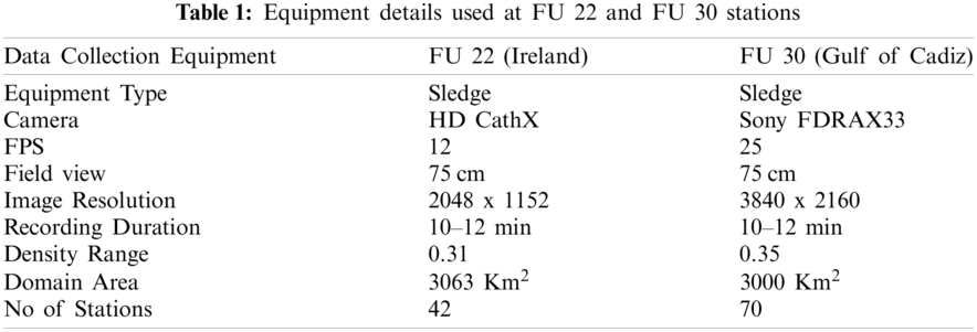
At FU 22, a sledge mounted with an HD video and stills CathX camera and lighting system at 75 ° to the seabed with a field view of 75 cm, confirmed using laser pointers were used [23]. High-definition still images were collected with a frame rate of 12 frames per second with a resolution of 2048 x 1152 pixels for a duration of 10 – 12 min. The image data was stored locally in a SQL server which was then analyzed using different applications. Fig. 5a shows the sledge used in data collection at FU 22.
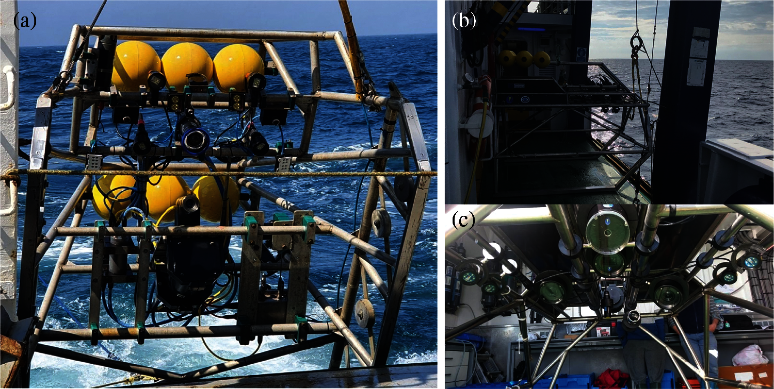
Figure 5: Sledge used in Ireland UWTV Survey (a) and sledge used in the gulf of cadiz UWTV survey: lateral VIew (b) and ventral view (c)
Similarly, at FU 30, a sledge was used to collect the data during the survey. Figs. 5a and 5c shows the sledge used in data collection at FU 30. The camera is mounted on top of the sledge with an angle of 45° to the seafloor. Videos were recorded using a 4 K Ultra High Definition (UHD) camera (SONY Handycam FDRAX33) with Lens of ZEISS® Vario-Sonnar 29.8 mm and optical zoom 10x. The sledge is equipped with a definition video camera and two reduced-sized CPUs with 700 MHz, 512 Mb RAM, and 16 GB storage. To record the video with good lighting condition four spotlights with independent intensity control is used. The equipment also has two-line laser separated 75 cm used to confirm the field of view (FOV) and a Li-ion battery of 3.7 V & 2400 mAh (480 Watt) to support the power of the whole system. Segments of 10–12-minute video duration was recorded at 25 frames per second, with a resolution of 3840 x 2160 pixels. The data were stored in hard disks and review later manually using by experts.
This paper obtained the data from the Smalls (FU 22) and Gulf of Cadiz (FU 30) UWTV surveys to conduct the experiments to detect Nephrops burrows automatically. Fig. 6a shows the map of MI-Ireland with stations carried out in 2018 to estimate the burrows. A station is a geostatistical location in the ocean where the Nephrops survey is conducted yearly. Fig. 6b shows the Gulf of Cadiz's map with stations carried out in 2018 and the Nephrops burrow density obtained using the manual count.
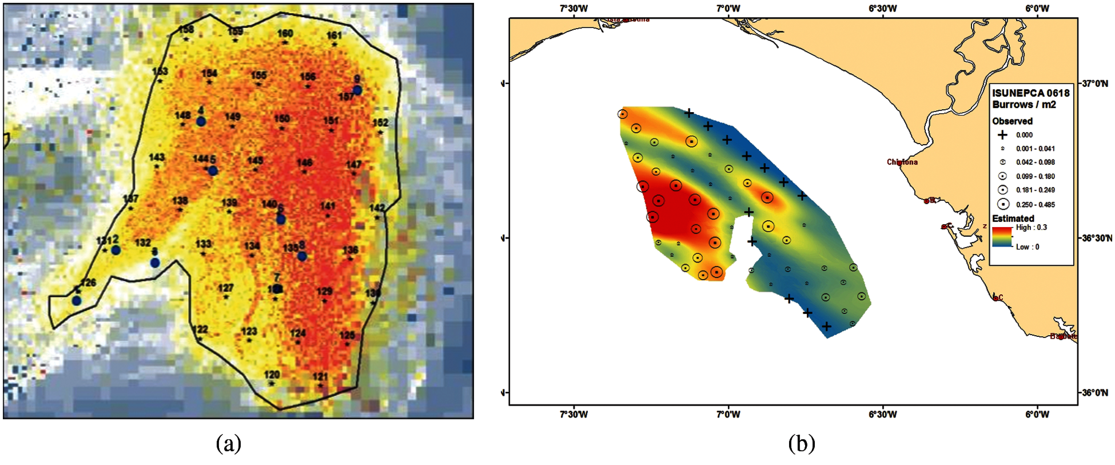
Figure 6: (a) Study area of Nephrops FU 22 at MI-Ireland in 2018 [23] (b) Study area of Nephrops FU 30 at the gulf of cadiz in 2018 survey showing the nephrops burrow density observed and geo-statistical nephrops abundance estimated [24]
The actual methodology used to count Nephrops is explained in introduction section and summary in Fig. 4. In this work, we replace the old paradigm of counting Nephrops and propose an automated framework that automatically detects and counts the number of Nephrops burrows with high speed and accuracy. Fig. 7 shows the high-level diagram of the proposed methodology. Video files are converted to frames using OpenCV and then images are manually annotated using the VOTT image annotation tool. The annotated data is verified by the marine experts before used for training the deep neural network. Fig. 8 shows the detailed steps of the research methodology used in this work.
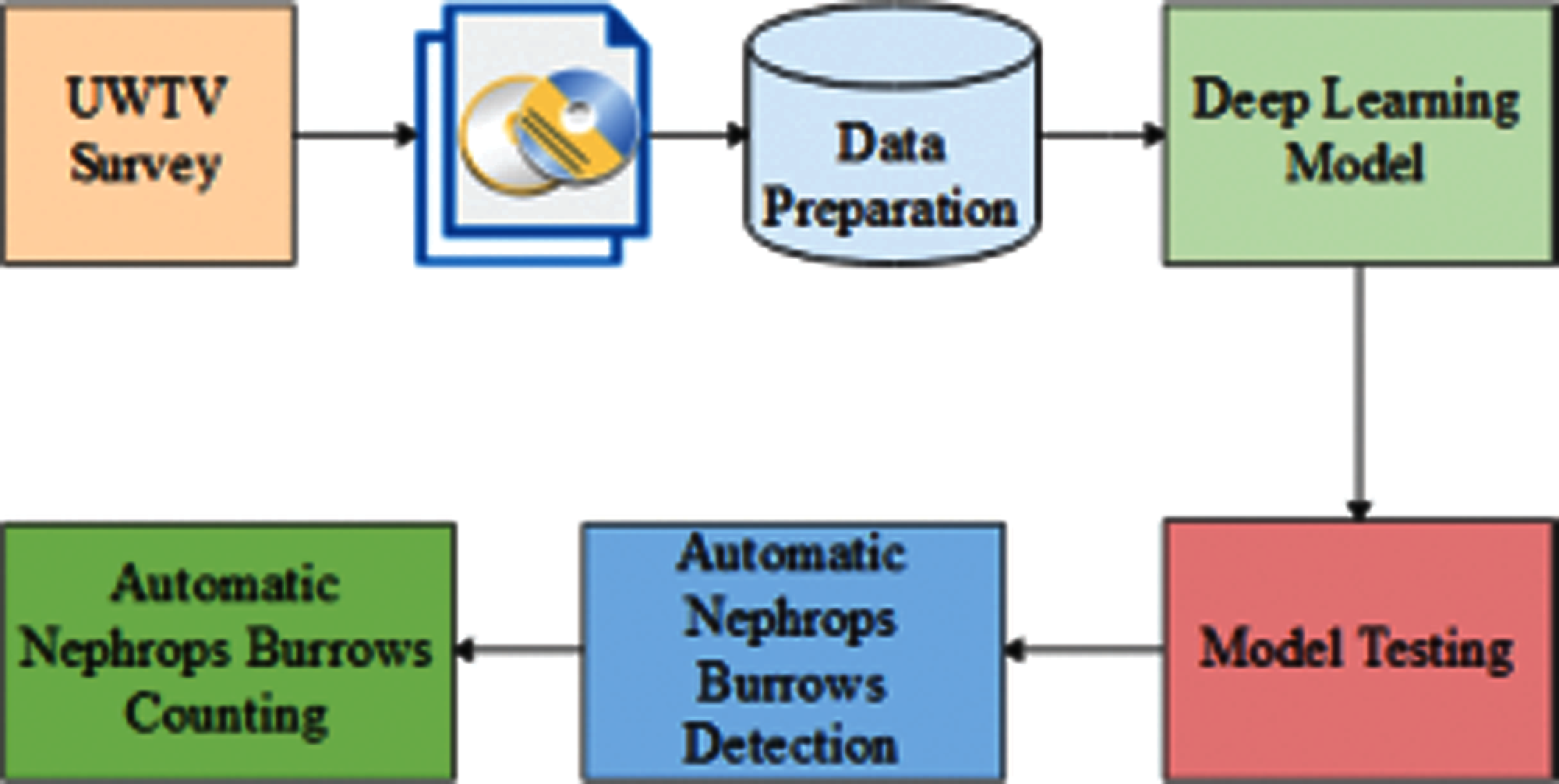
Figure 7: Block diagram of proposed methodology
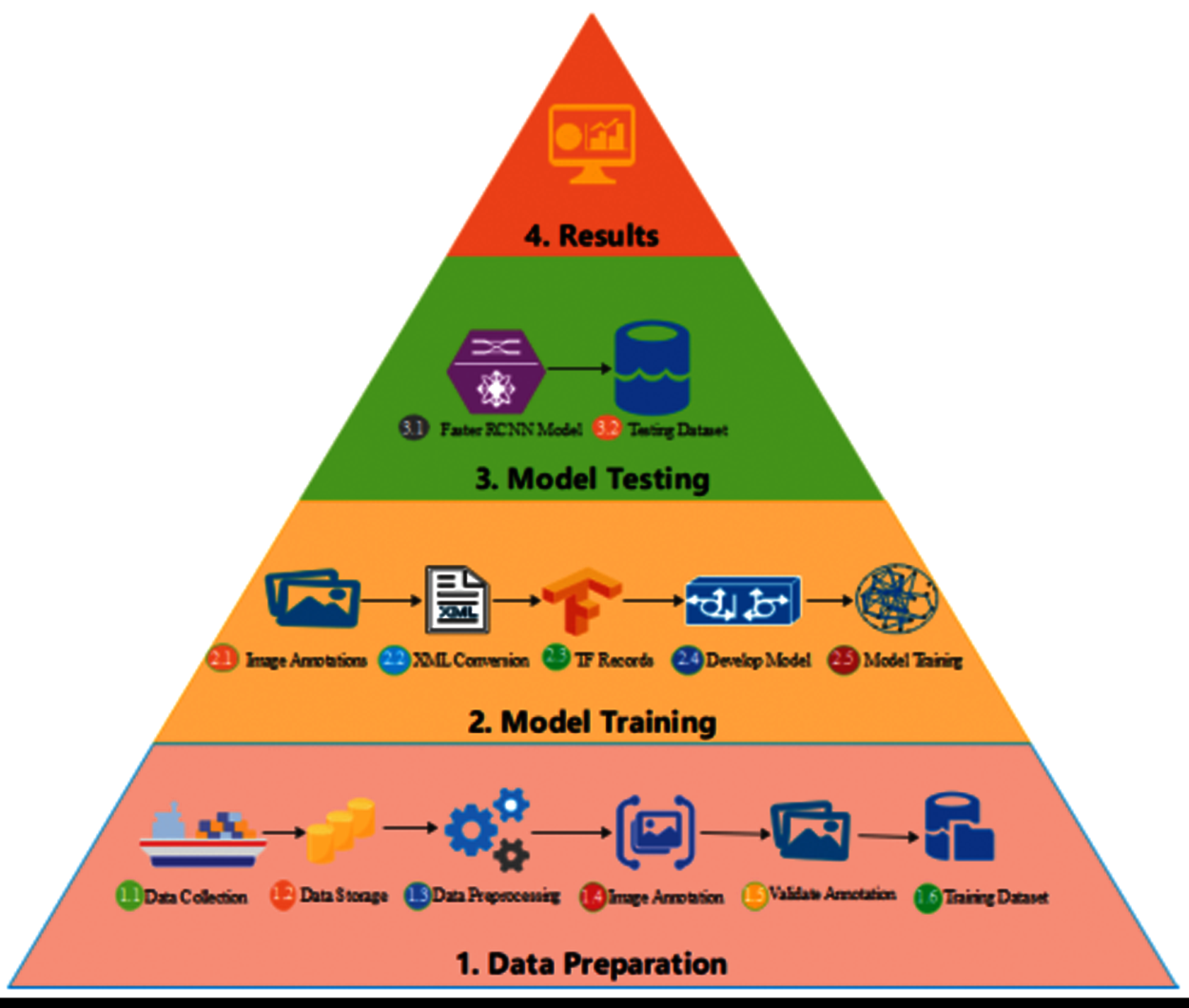
Figure 8: Architecture of proposed methodology
Tab. 1 shows the techniques and equipment used in collecting the data from FU 22 and FU 30 stations.
At FU 22, a total of 42 UWTV stations were surveyed in 2018. Out of 42, seven stations were used for data preparation. The 10–12 min video were recorded at different frame rates ranging from 15 fps, 12 fps, and 10 fps at Ultra HD. Also, the high-definition images were captured with the camera. The images were recorded with a resolution of 2048 x 1152 pixels. Out of thousands of recorded images, a total of 1133 high-definition images were manually annotated from FU 22. Figs. 9a and 9b shows the high definition still images from the 2018 UWTV survey HD camera. In the top image, it can be seen a burrow system composed of three holes in the sediment, whereas in the bottom image, a single Nephrops individual is seen outside the burrows. Illumination is better near the center of field view and decreases to the borders of the images. The camera angle shows 75 degrees with a ranging laser (red dots) on the screen. A Nephrops burrow system may be composed of more than one entrance, and in this paper our focus is to detect the individual Nephrops burrows entrances.
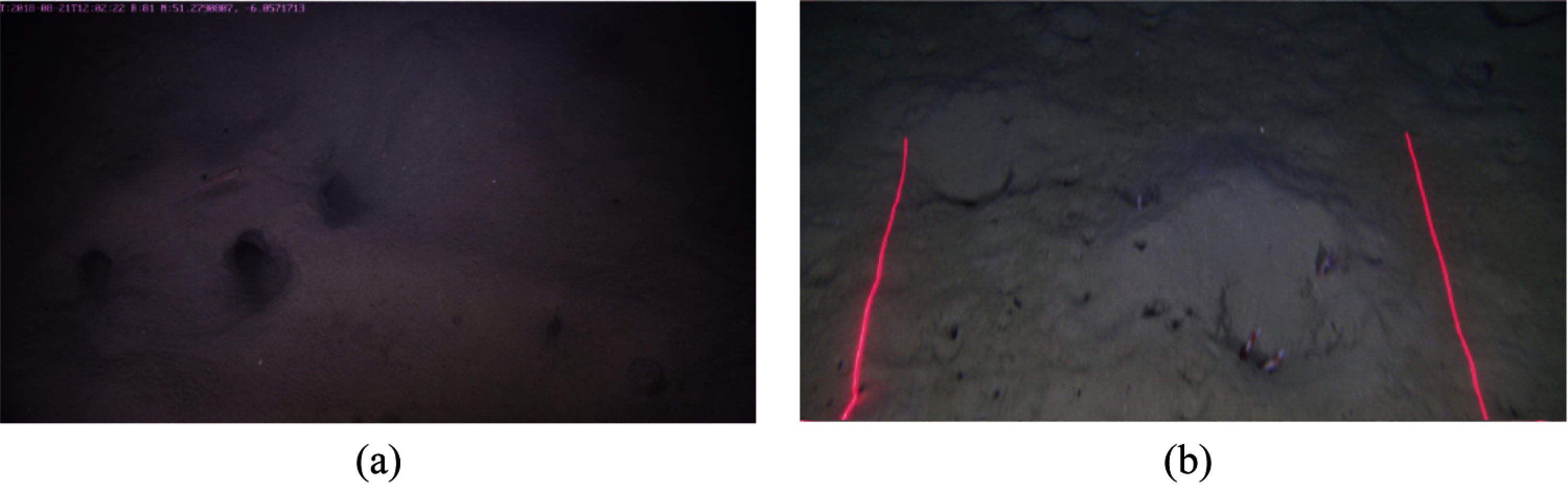
Figure 9: (a) High definition still images from 2018 UWTV survey for FU22 station (b) High definition still images from 2018 UWTV survey for FU30 station
At FU 30, the videos are recorded at 25 frames per second in good lighting condition. Video footage of 10–12 min has been recorded by every station at FU 30. A total of 70 UWTV stations were surveyed in 2018. Out of 70 surveyed stations, 10 were rejected due to poor visibility and lighting conditions. We selected seven stations for our experimentation which have good lightening condition, low noise and few artifacts, higher contrast, and high density of Nephrops burrows. The data from seven stations are considered for annotations. So, each video is around 15,000–18,000 frames. A total of 105,000 frames were recorded from seven different stations of the 2018 data survey. Figs. 9c and 9d shows the high-definition images from the 2018 UWTV survey of FU 30. FU 30 images show better illumination (in terms of contrast and homogeneity) than FU 22. Pink lines on the images correspond to red laser lighting to 75 cm width searching areas (the red color is seen pink due to the distortion produced by different attenuation of light wavelength in water.
Data collected from FU 22 and FU 30 is converted into frames. The collected data set has a lot of frames with low and non-homogeneous lightning and poor contrast. The frames that do not contain any burrows or poor visibility are discarded during the annotation phase, and consecutive frames with similar information are also discarded.
Image annotation is a technique used in Computer Vision to create training and testing ground truth data, as this information is required by supervised deep learning algorithms. Usually, any object is annotated by drawing a bounding box around it.
Currently, the marine experts that work with Nephrops burrows are not using any annotation tool to annotate Nephrops burrows, as this is a time-consuming job. In this phase, we annotate the images to overcome this challenge, and all recorded annotations are validated by the marine experts from Ireland and Cadiz institutes before training and testing processes.
We adopt the mechanism to annotate the burrows manually in the Microsoft VOTT image annotation tool [19], using Pascal VOC format. The saved XML annotation file contains image name, class name (Nephrops), and bounding box details of each object of interest in the image. As an example, Fig. 10 shows two screenshots from the FU 22 and FU 30 UWTV surveys that are manually annotated.

Figure 10: Manual annotation in a frame from (a) FU 22 and (b) FU 30 UWTV survey using VOTT
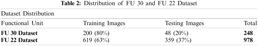
Tab. 2. shows the number of ground truth burrow holes annotated of each station from the FU 22 and FU 30 UWTV surveys that will be used in the model training and testing. A total of seven stations are annotated for FU 30, and seven stations are for FU 22. A total of 248 images are annotated for seven stations of FU 30, and 978 images were annotated for seven FU 22 stations before validation stage. In general, there is a higher density of Nephrops burrows from FU 22 compared to FU 30 which is a factor of population dynamics.
The annotated images are validated by marine sciences experts from Spain and Ireland. The validation of annotation is essential to obtain high quality ground-truth information. This process took a long time as confirming every single annotation is time consuming and sensitive job. After validating each annotation, a curated dataset is used for training and testing the model.
3.1.5 Preparation of Training Dataset
The annotated images are recorded into XML files and converted to TFRecord files, which are a sequence of binary strings that TensorFlow requires to train the model. The dataset is divided into two subsets: train and test. Tab. 2 shows the distribution of the subsets for each dataset.
To train a model, we used Convolution Neural Network (CNN). Instead of train the network from scratch, we utilized transfer learning [25] to fine-tune the Faster R-CNN Inceptionv2 [21] and MobileNetv2 [22] models in TensorFlow [25]. Inceptionv2 is one of the architectures that have a high degree of accuracy. The basic design of Inceptionv2 helps to reduce the complexity of CNN. We used a pre-trained version of the network model trained on the COCO dataset [26]. Inceptionv2 is configured to detect and classify only one class (c = 1), namely “Nephrops”. When training the network, the “Momentum” optimizer [27] was used with a decay of 0.9. The momentum method allows us to solve the gradient descent problem. We trained a network with a learning rate of 0.01 with a batch size of 1. The Maxpool kernel size and Maxpool stride value are set to 2. The gradient clipping [28] was set with a threshold value of 2.0. (The gradient value too high and too low will lead to insatiability of the model). The Softmax activation function is used in the model. Tab. 3 shows the parameter list and their values used in the Inceptionv2 model. The model is evaluated after every 10k iterations. A total of 70k iterations were performed. The box predictor used in the Inceptionv2 model was Mask RCNN. Fig. 11 shows the layer-by-layer details of the Inceptionv2 model.
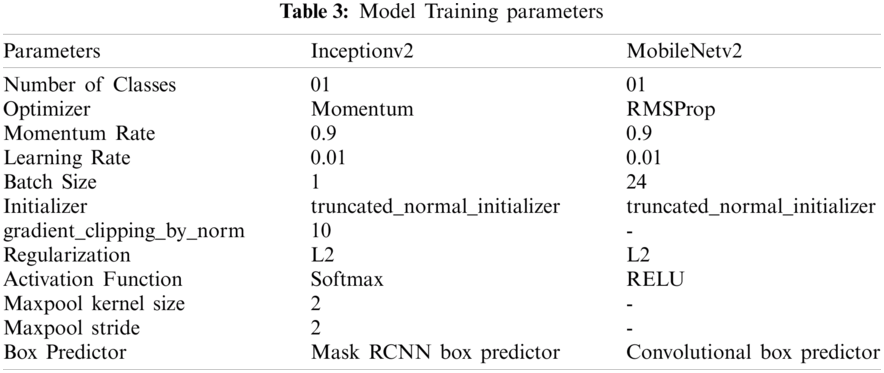
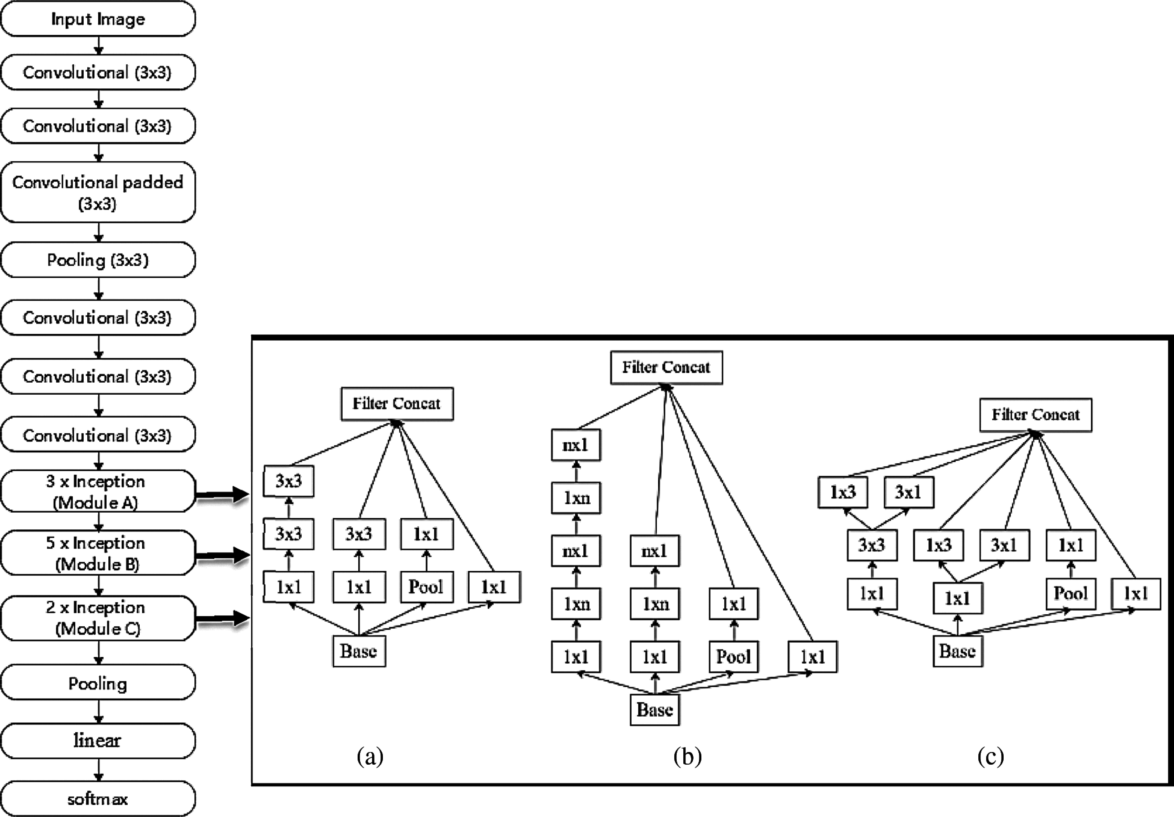
Figure 11: Inceptionv2 layers and architecture
The MobileNetv2 CNN architecture was proposed by Sandler et al. [29]. One of the main reasons to choose the MobileNetv2 architecture was the relatively small training dataset from FU30. This architecture optimizes the memory consumption and execution speed at minor errors. MobileNetv2 architecture has depth-wise separable convolution instead of conventional convolution. This architecture initially has a convolution layer with 32 filters, followed by 17 residual bottleneck layers (Fig. 12). Our experiments achieved the best model result with RMSProp [30] momentum with a decay of 0.9. We used a learning rate of 0.01, a batch size of 24 and a truncated normal initializer. The L2 regularization is used with Rectified Linear Unit (ReLU) as an activation function. The box predictor used in the MobileNet model was the Convolutional box predictor. Tab. 3 shows the parameter list and their values used in the MobileNetV2 model.
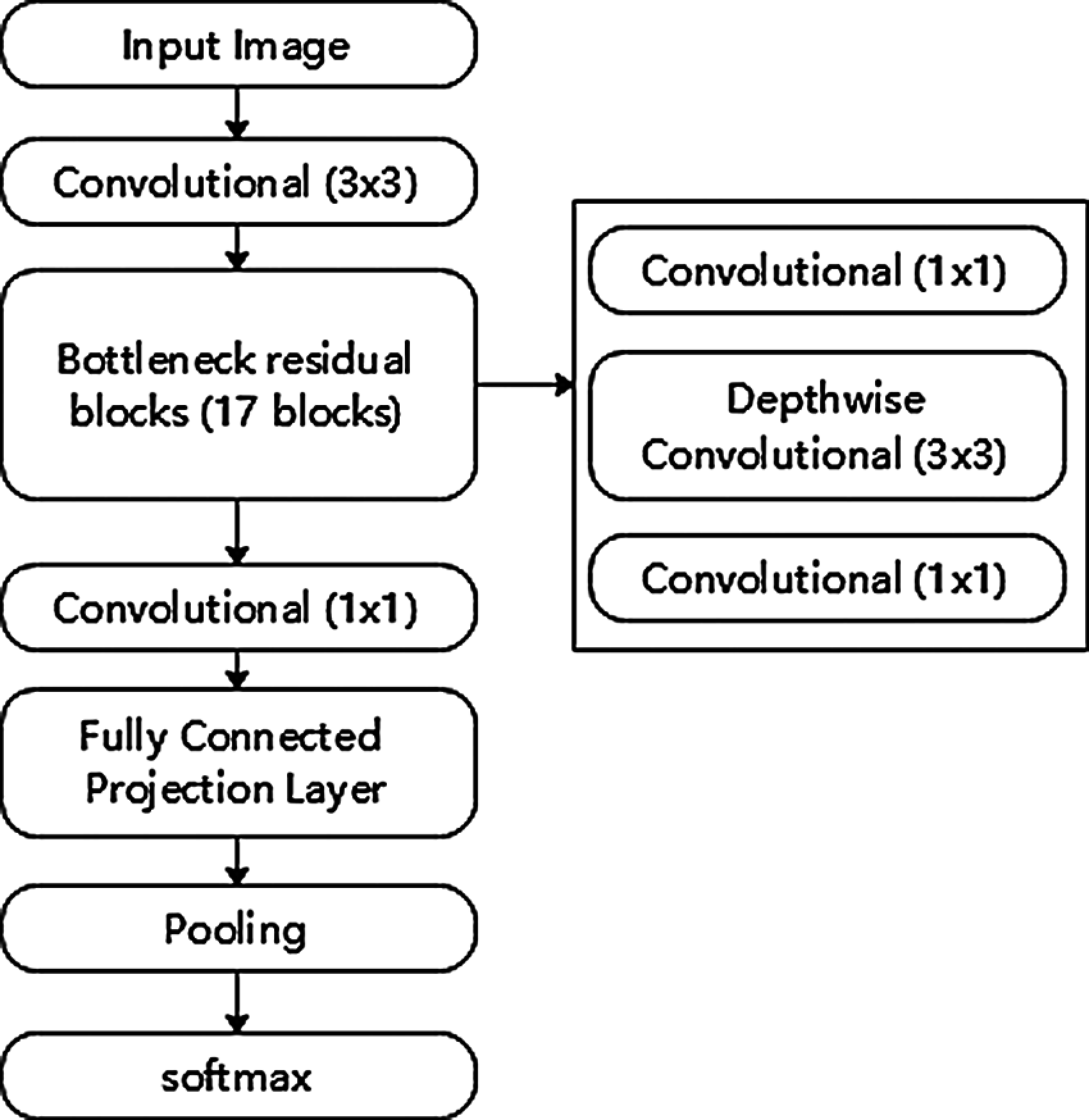
Figure 12: Mobilenetv2 model architecture
We conducted the model training, validation, and testing on a Linux Machine powered by an NVIDIA TitanXP GPU. We created multiple combinations for model training, i.e., trained separate model for Cadiz and Ireland dataset, training a model by combining both datasets, and training and testing with different datasets. For FU30, 200 images are used, and for FU22, 619 images are used for training the model. Both the Inception and MobileNet models used two classes (one for Nephrops and one as background), L2 regularization for training and were trained with 70k steps. MobileNetv2 is two times quicker in training as compared to the Inceptionv2 model.
Precision can be seen as how robustly the model identifies Nephrops burrows’ presence, and Recall is the rate of TP over the total number positives detected by the model [31]. Generally, when the recall increases, precision decreases, and vice versa, so precision vs. recall curves P(R) are valuable tools to understand model behavior. To quantify how accurate the model with a single number, the mean average precision (mAP), defined in Eq. (1), is used.
In our problem, ground truth annotation and model findings are rectangular areas that usually don't fit perfectly. In this paper, it is considered a TP detection if both areas overlap more than 50%. This is computed by Jaccard index J, defined in Eq. (2)
A and B are the set of pixels in the truth annotation and model finding rectangular areas, respectively, and . means the number of pixels in the set. When J ≥ 0.5, a TP is detected, but if J < 0.5, detection fails with an FN. Using this methodology, P and R values are calculated, and mAP is used as a single number measure of the goodness of the model. Usually, this parameter is named mAP50, but we used mAP for simplicity in this paper.
Models were trained using a random approximately 70–75% sample of the annotated dataset. The remaining is used for testing. We measured the training performance by monitoring the over-fitting of the model. We recorded the turning checkpoints after every 10k iterations and computed the mAP50 on the validation dataset. The model is evaluated using mAP, precision and recall curve, and by visual inspection of the images with automatic detections. Fig. 13 shows the model evaluation life cycle.
The model is tested to assess the performance. We tested our model against some unseen images from the FU 30 and FU 22 datasets and evaluated the model's performance.
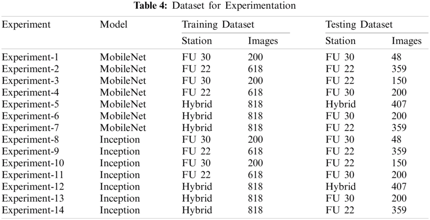
In this section, we evaluate the performance of different networks both in qualitative and quantitative ways. To detect the Nephrops burrows automatically, multiple experiments are performed. We trained the models on three datasets. The first dataset purely contains FU 30 images. The second dataset contains the images from the FU 22 dataset, and the third is the hybrid dataset that contains the images from both datasets. Fourteen different combinations of set of experiments are performed. Each set is iterated seven times. So, 98 experiments were carried out. The details of the experiments are shown in Tab. 5.
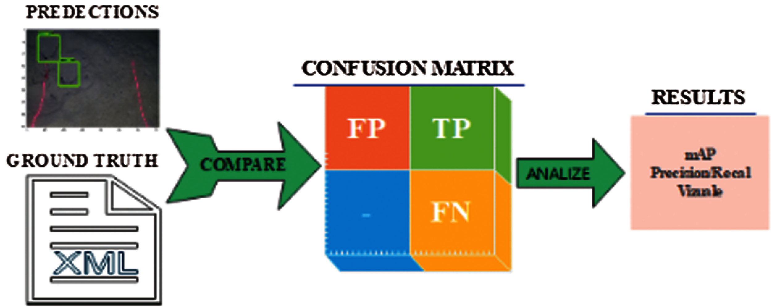
Figure 13: Model evaluation life cycle
The MobileNet and Inception models used 200 images from the FU 30 dataset for training the model, while 48 images for testing the models. Similarly, these models used 618 images from FU 22 dataset for training and 359 images for testing. The MobileNet and Inception models that were trained using the FU 30 data set and were tested using FU 22 dataset used 200 images for training the model and 150 images for testing. The models that used the FU 22 data set for training and FU 30 data set for testing used 618 images to train the model while 200 images were for testing. Finally, the MobileNet and Inception models that used the hybrid data set for training and testing used 818 images for training the model while 407 images for testing the model. Tab. 4 shows the details of the data set used for these experiments.

We trained both MobileNet and Inception models over 70k iterations. The models’ performance is reported after every 10k iterations and achieves an excellent precision on the trained dataset, as shown in Fig. 14.
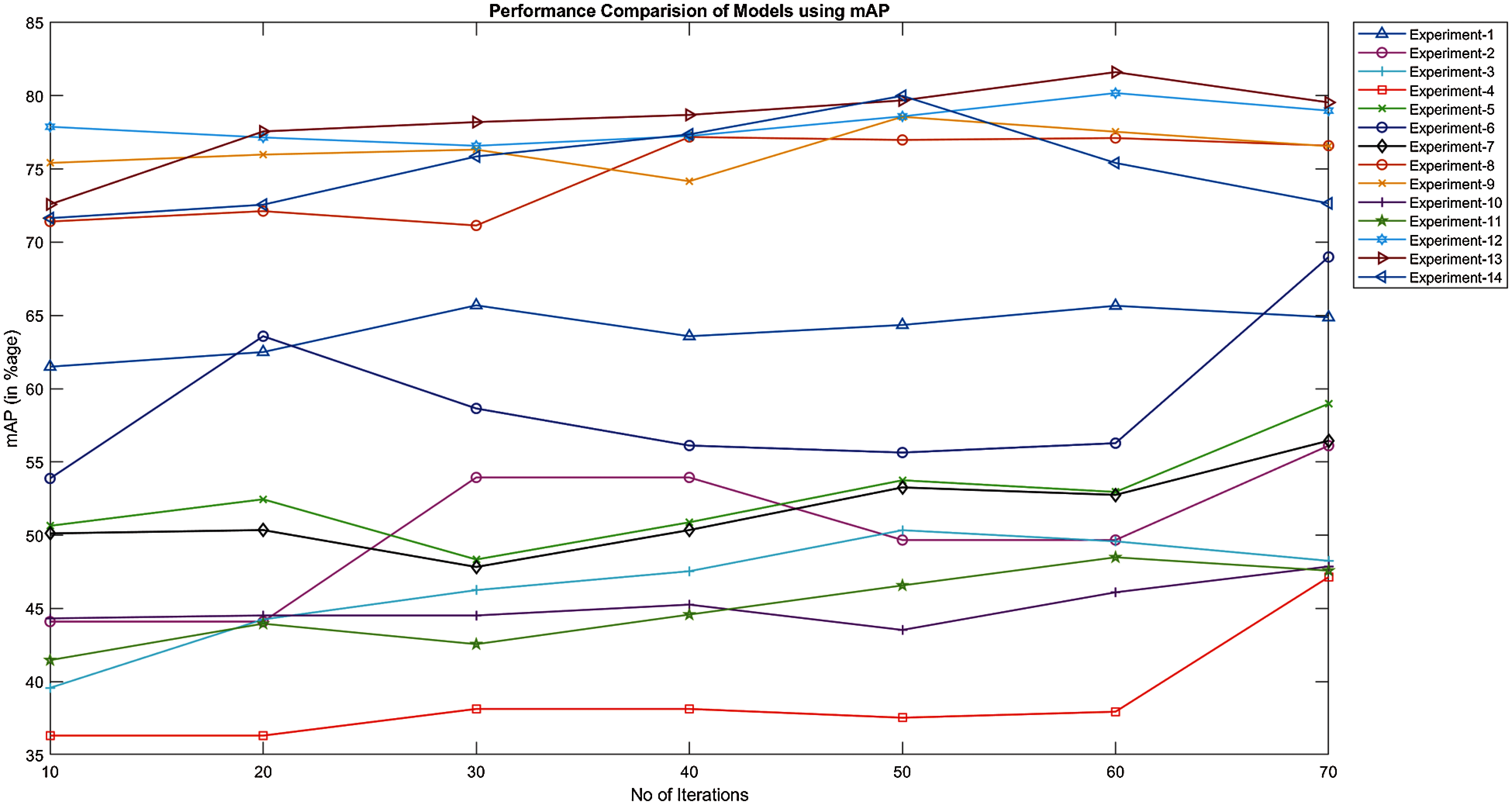
Figure 14: Mean average precision of models trained and tested by FU 22 and FU 30 stations
We evaluate the performance in terms of mAP, which is a prevalent metric in measuring object detectors algorithms’ accuracy like Faster R-CNN, SSD, etc. Average precision calculates the average precision value for recall value over 0 to 1. Precision is the measurement of prediction accuracy, while Recall measures the positive predictions. We computed the mAP with the dataset of Nephrops from FU22 and FU30 stations over 100k iterations.
Fig. 14 shows the results obtained by MobileNet and Inception models. These models are trained and tested by the different FU 30 and FU 22 data sets. The best mAP is 81.61% achieved by the Inception model trained using the Hybrid data set while tested by the FU 30 data set (experiment-13). Also, the mAP of 79.99% is achieved when the Inception model is trained and tested using hybrid data sets (experiment-12). As expected, the MobileNet and Inception models do not Perform very well when trained by the FU 30 data set and tested by FU 22 data set and vice versa, as it can be seen in Fig. 14, where minimum value of mAP in these models was 47.86%, 48.49%, 50%, and 57.14%.
As it can be seen in Fig. 14, mAP for most of the experiments increases with the number of iterations until 60k iterations. However, after this value, performance does not increase or became a bit erratic, and this behaviour could be explained because the overfitting of the model. It is also shown in the figure that Inception models show a more stable performance with the iteration number than the MobileNet. In summary, these results clearly show that the mAP of the Inception model is better than the MobileNet for this problem.
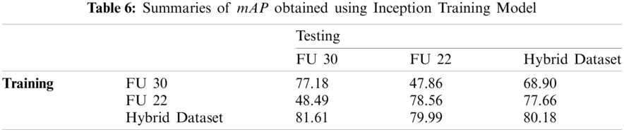
Tabs. 5 and 6 show the maximum mAP obtained by MobileNet and Inception models, respectively. In the first experiment, both models were trained using the FU 30 data set and tested by FU 30, FU 22, and hybrid dataset. While in the second experiment, the models were trained using the FU 22 data set and tested by FU 30, FU 22, and hybrid dataset. Finally, the model was trained using hybrid dataset and tested by FU 30, FU 22, and hybrid dataset separately. The maximum mAP obtained using the MobileNet model is 75.12% that is when the model is trained using the FU 22 data set and tested by the FU 22 data, but the results obtained by Inception training are much better as we achieved the mAP over 80% after training the model by the combined data set of FU 30 and FU 22.
We also evaluate the performance of the models using precision-recall curves. For model evaluation, TP, FP, and FN annotations are calculated.
Fig. 15 shows the precision and recall of MobileNet (left side), and Inception (right side) models trained and tested by the FU 30 data set after 70k iterations.
Fig. 16 shows the precision and Recall of MobileNet (left side), and Inception (right side) models trained and tested by FU 22 data set after 70k iterations. Similarly, Fig. 17 shows the precision and recall of MobileNet (left side), and Inception (right side) models trained and tested by FU 30 and FU 22 data set after 70k iterations.
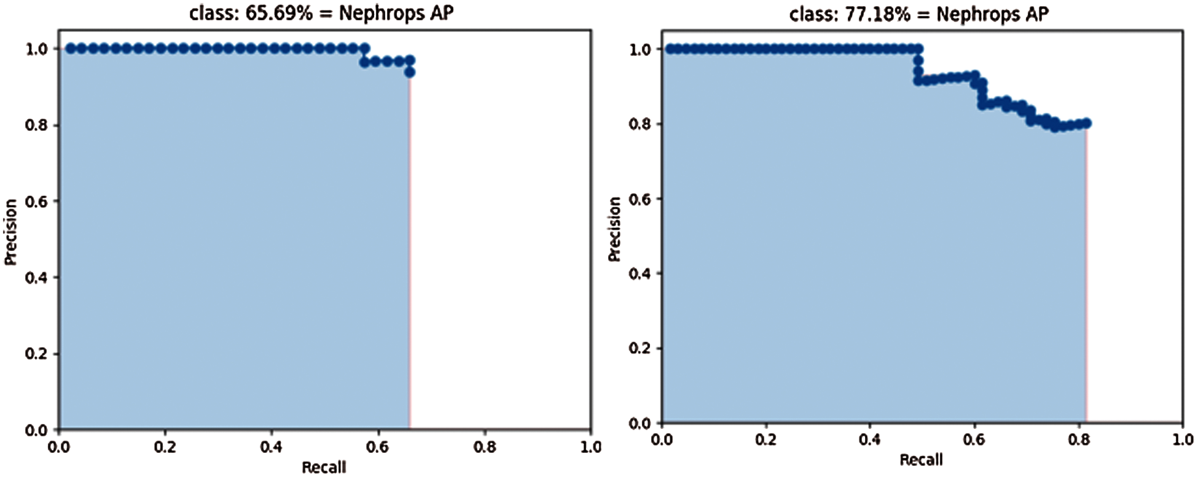
Figure 15: Precision-recall curve of mobilenet (left) and inception (right) using FU 30 dataset
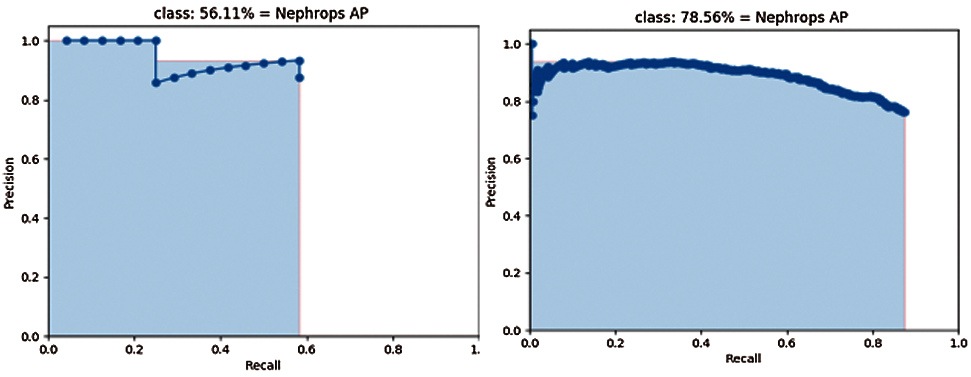
Figure 16: Precision-recall curve of mobilenet (left) and inception (right) using FU 22 dataset
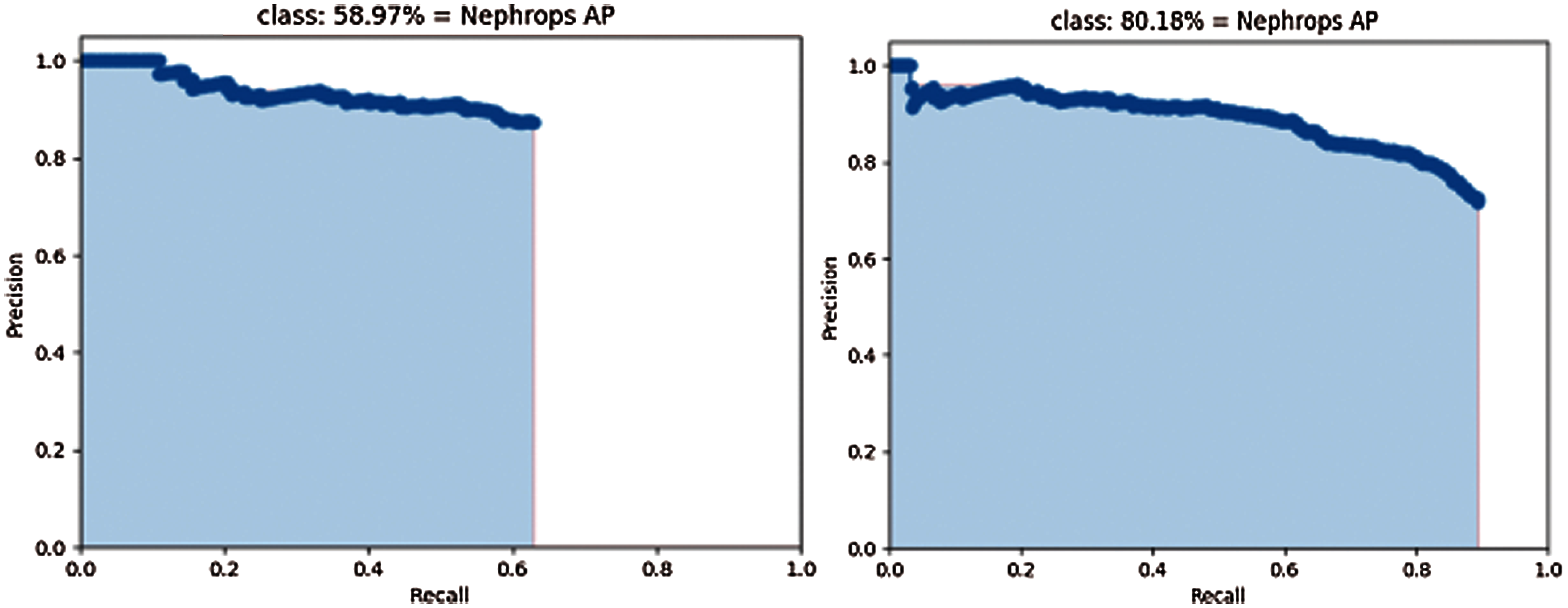
Figure 17: Precision-recall curve of mobilenet (left) and inception (right) using Hybrid dataset
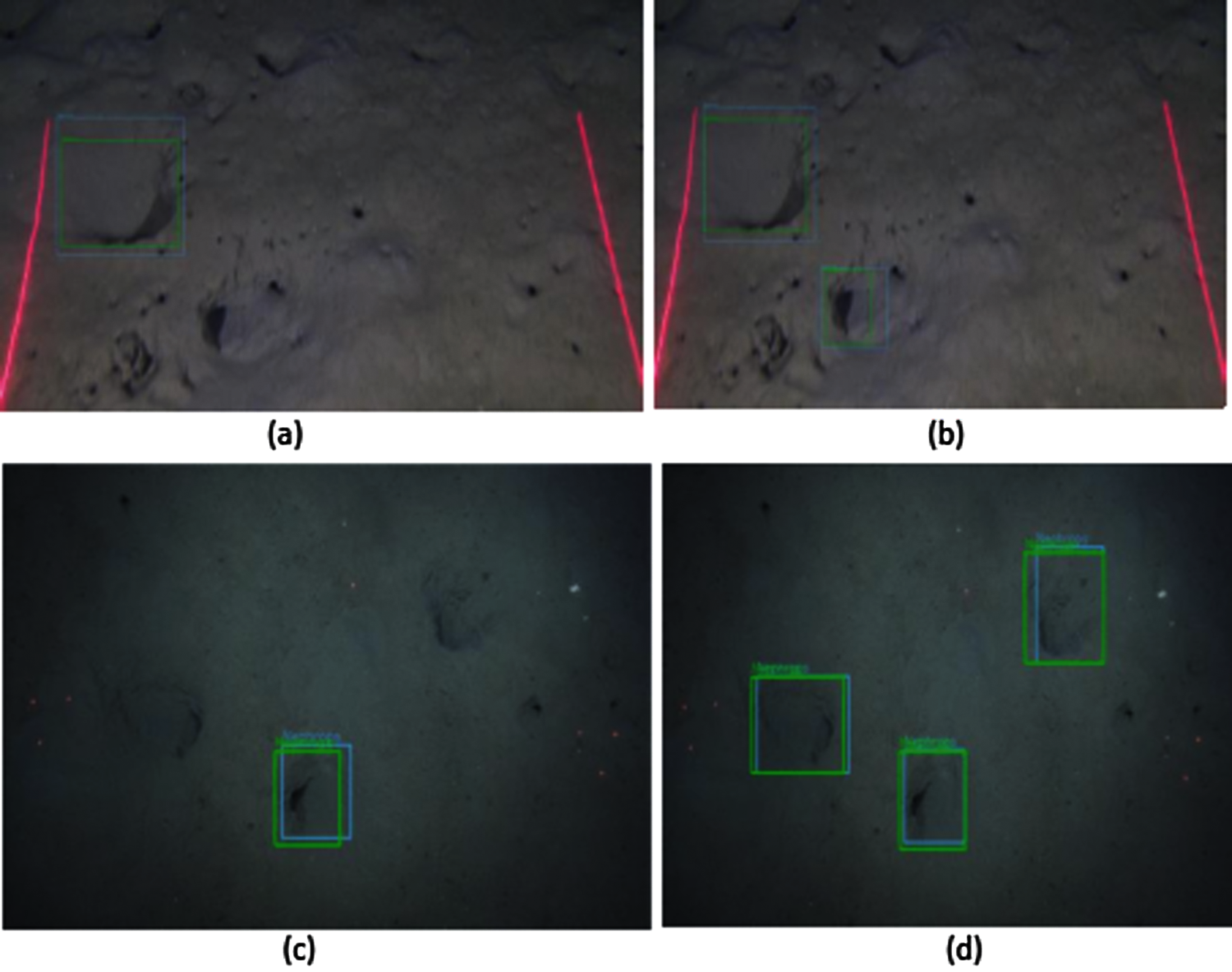
Figure 18: Nephrops burrows detections (a)(b) FU30-Mobilenet vs. FU30-Inception (c)(d) FU22-Mobilenet vs. FU22-Inception
The mAP values could be interpreted as the area under these curves, but the behaviour of models is different. With the Inception model, precision values are close to those obtained with MobileNet model, but higher Recall values can be computed, because a lower number of FN, which results in higher values of mAP.
In this section, we will qualitatively analyze the performance of different models on different datasets. The visualization results are from MobileNet and Inception models, trained and tested using a different combination of the FU 30 and FU 22 datasets.
Figs. 18–21 shows the detections of Nephrops burrows using MobileNet and Inception models, with a different combination of FU30 and FU22 datasets. The green bounding boxes on the images shown in this section are the TP detections by the trained model. The blue bounding boxes show the correct ground annotations. The red bounding boxes are the FP detections of trained models. Also, the results show the detections with a confidence level ranging from 97% to 99%.
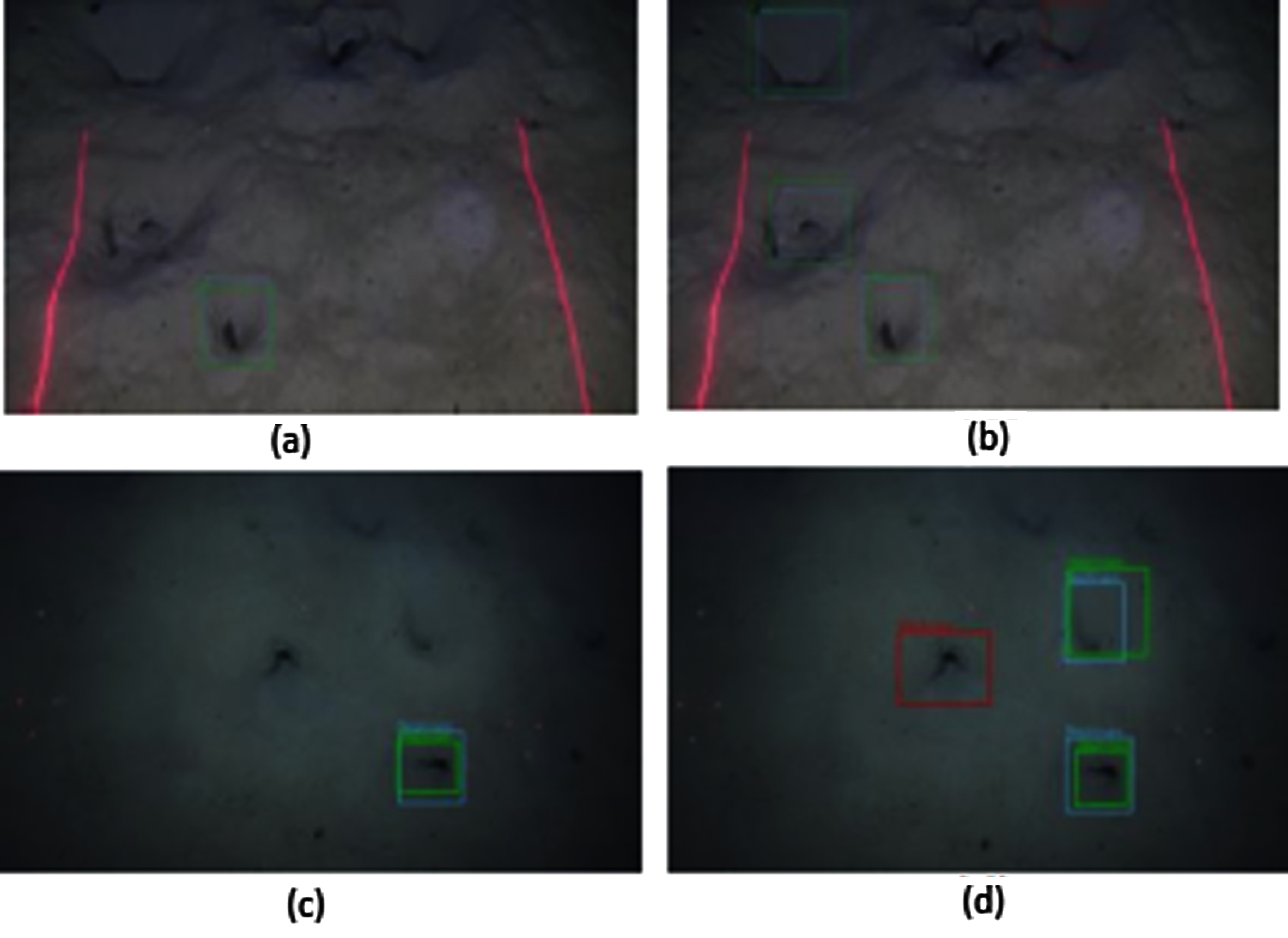
Figure 19: Nephrops burrows detections by model using hybrid dataset (a)(b) FU30-Mobilenet vs. FU30-Inception, (c)(d) FU22-MobileNet vs. FU22-Inception
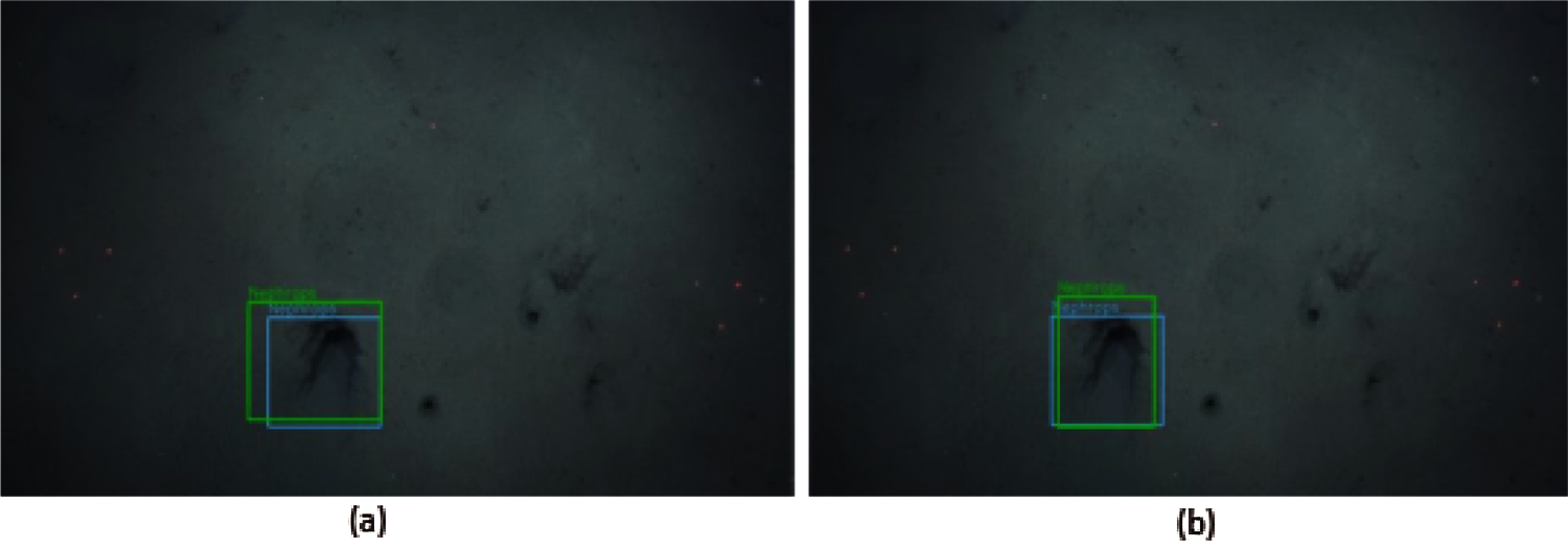
Figure 20: Nephrops burrows detections by model trained by FU30 and tested by FU22 dataset (a) FU22-MobileNet, (b) FU22-Inception
Figs. 18a and 18b show the detections on the FU 30 data set obtained with MobileNet and Inception trained models. In this example, MobileNet model detects one TP Nephrops burrows while the inception model detects two. Figs. 18c and 18d show the detections on FU 22 dataset. In both images, there are more TP detections with the Inception than with MobileNet trained model.
Fig. 19 shows the FU 30 and Inception models’ results trained by both the FU 30 and FU 22 data set. Fig. 19a shows only one TP detection of the FU 30 data set with the MobileNet model while, Fig. 19b shows the three TP and one FP detections of burrows by the Inception model. Similarly, Figs. 19c and 19d shows a significant difference in TP Nephrops burrows detections in MobileNet and Inception model on the FU 22 data set.
Fig. 20 shows the detections of Nephrops burrows from the FU 22 data set. The MobileNet and Inception models are trained by the FU 30 data set and tested using the FU 22 dataset. Figs. 20a and 20b show the detections using MobileNet and Inception models, respectively. Both models do not show any significant change in detections.
In Fig. 21, the results are obtained using the model trained by the FU 22 data set and tested by the FU 30 data set. The image is shown in Fig. 21a is the result obtained by the MobileNet model, while Fig. 21b shows the results by the Inception model. The MobileNet model detects one TP while the Inception model detects one TP and one FP.
Fig. 22 shows the MobileNet and Inception models, trained by FU 30 data and tested by both FU 30 and FU 22 data. Fig. 22a uses the MobileNet model and detects one burrow, while Fig. 22b detects two Nephrops burrows from the same image using Inception as a training model. In Figs. 22c and 22d, the Nephrops burrows are detected from the FU 22 data set using MobileNet and Inception training models. The Inception model detects one TP while the model trained by MobileNet detects no burrows.
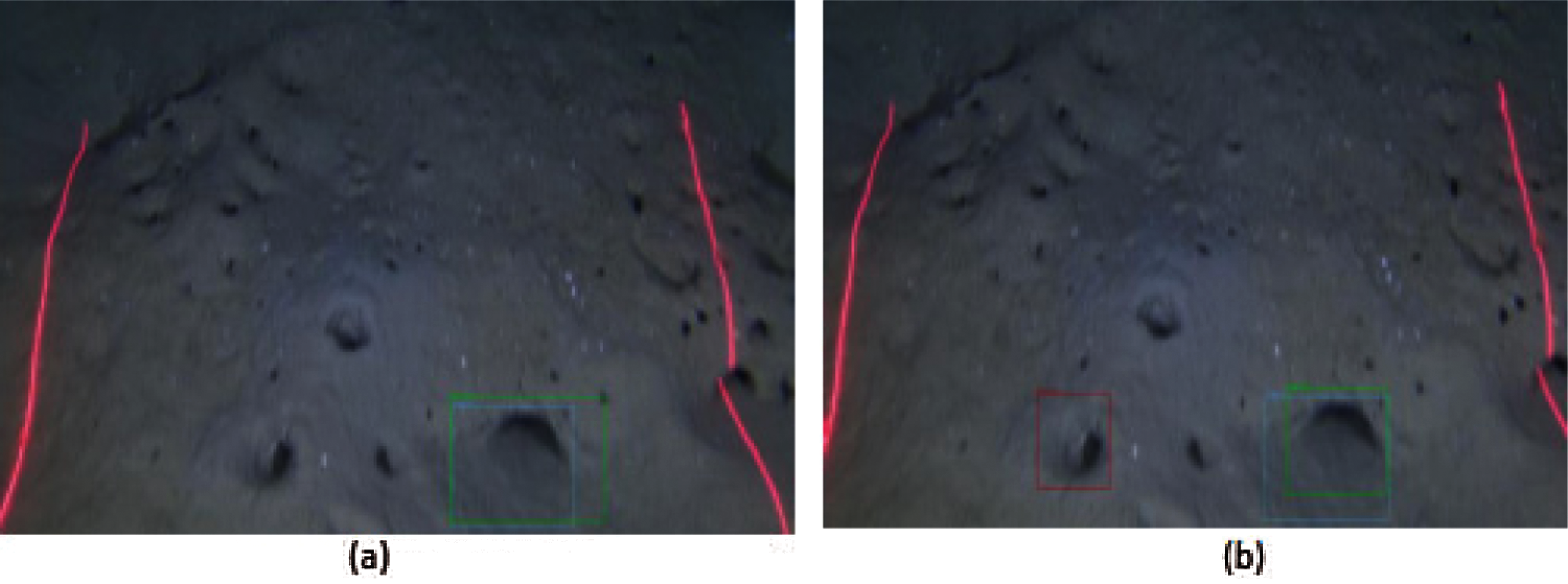
Figure 21: Nephrops burrows detections by model trained by FU 22 and tested by FU 30 dataset (a) FU 30-MobileNet, (b) FU 30- Inception
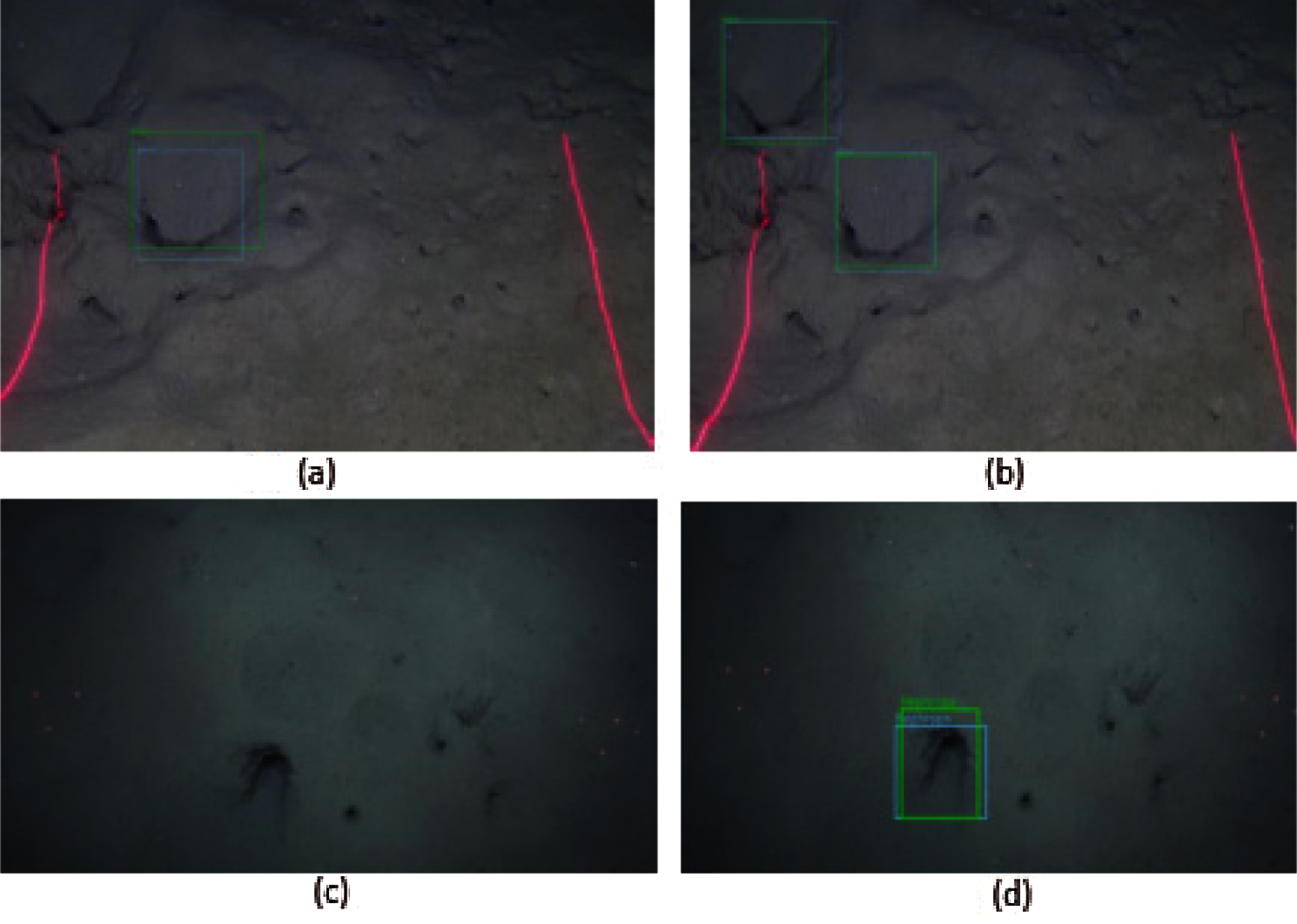
Figure 22: Nephrops burrows detections by model trained by FU30 and tested by hybrid dataset (a)(b) FU30-MobileNet vs. FU30-Inception, (c)(d) FU22-MobileNet vs. FU22-Inception
Fig. 23 shows the MobileNet, and Inception models trained by FU 22 data and tested by hybrid data set. The results did not show any significant difference when the FU 30 data set tests both the models, as shown in Fig. 23. Still, when the models are tested using the FU 22 data set, the Inception model detects two TP. In contrast, MobileNet only detects one, as shown in Figs. 23c and 23d.
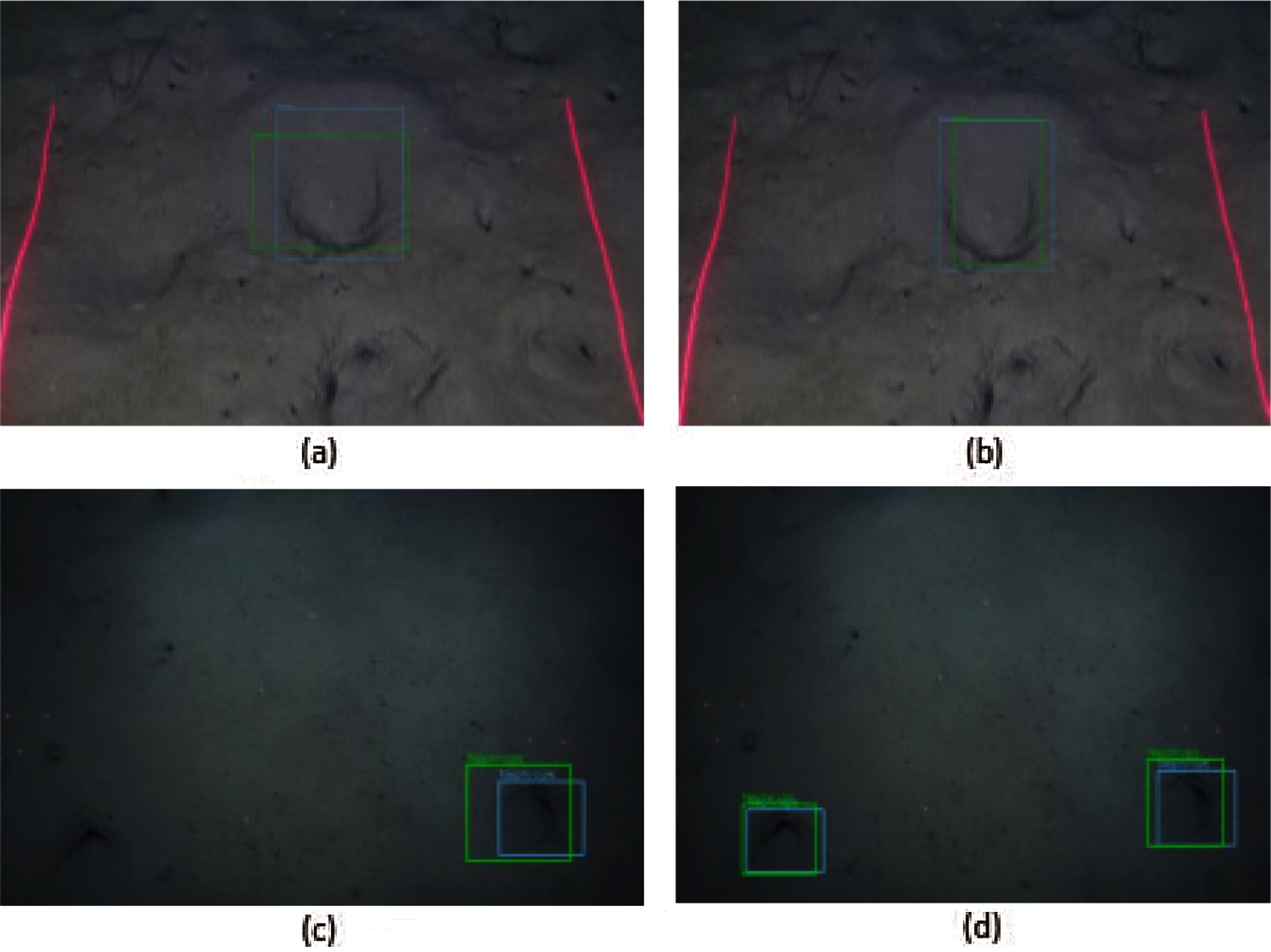
Figure 23: Nephrops burrows detections by model trained by FU22 and tested by hybrid dataset (a)(b) FU30-MobileNet vs. FU30-Inception (c)(d) FU22-MobileNet vs. FU22-Inception
The visualization results clearly show that the Inceptionv2 model is much better in precision and accuracy. The model trained by Inception detects more True Positives as compared to MobileNet. Visualization of results also helps to understand the models’ errors and improve them in future work.
Our results prove that deep learning algorithms are a valuable and effective strategy to help marine science experts in the assessment of the abundance of Nephrops norvegicus specie when underwater video/image surveys are carried out every year, following ICES recommendations. The automatic detection algorithms could replace in a near future the tedious and sometimes difficult manual and human review of data, which is nowadays the standard procedure, with the promise of better accuracy, coverage of bigger areas in sampling and higher consistency in the assessment.
In future work, we will plan to use a bigger curated dataset from FU22 and FU30 areas with expert's annotations to improve the training of the Deep Learning network and validate the algorithm with data from other areas, which usually shows different habitats and relation with other marine species, and in image processing point of view, also differences in image quality, video acquisition procedures, and background textures. At the same time, the accuracy of detection could be obtained with the use of more dense object detection models and novel architectures. Finally, we will plan to correlate the spatial and morphological distribution of burrows holes to estimate the number of burrows complexes that are present and compare with human inter-observer variability studies.
Acknowledgement: We thank the Spanish Oceanographic Institute, Cádiz, Spain, and Marine Institute, Galway, Ireland for providing the dataset for research.
Funding Statement: Open Access Article Processing Charges has been funded by University of Malaga.
Conflicts of Interest: The authors declare that they have no conflicts of interest to report regarding the present study.
1. T. Rimavicius and A. Gelzinis, “A comparison of the deep learning methods for solving seafloor image classification task,” Communications in Computer and Information Science, vol. 756, pp. 442–453, 2017. [Google Scholar]
2. H. Qin, X. Li, Z. Yang and M. Shang, “When underwater imagery analysis meets deep learning: A solution at the age of big visual data,” in Proc OCEANS'15 MTS/IEEE, Washington, DC, USA, pp. 1–5, 2015. [Google Scholar]
3. “EU Council Regulation 2018/120 (2018, Jan 18). “Fixing for 2018 the fishing opportunities for certain fish stocks and groups of fish stocks, applicable in union waters and, for union fishing vessels, in certain non-union waters, and amending regulation (EU) 2017/127”, [Online]. Available: http://data.europa.eu/eli/reg/2018/120/oj. [Google Scholar]
4. M. Jiménez, I. Sobrino and F. Ramos, “Objective methods for defining mixed-species trawl fisheries in spanish waters of the gulf of cádiz,” Fisheries Research, vol. 67, no. 2, pp. 195–206, 2004. [Google Scholar]
5. ICES. 2017, “Report of the Workshop on Nephrops Burrow Counting,” WKNEPS 2016 Report, Reykjavík, Iceland. ICES CM 2016/SSGIEOM:34, International Council for the Exploration of the Sea, Copenhagen V, Denmark, pp. 9–11, November 2016. [Google Scholar]
6. A. Leocádio, A. Weetman and K. Wieland, “Using UWTV surveys to assess and advise on nephrops stocks,” ICES Cooperative Research Report, no. 340. pp. 49, 2018. [Online]. Available: DOI https://10.17895/ices.pub.4370. [Google Scholar]
7. ICES, CIES, 2021. [Online]. Available: https://www.ices.dk/about-ICES/Pages/default.aspx. [Google Scholar]
8. M. Aristegui, J. Aguzzi, C. Burgos, M. Chiarini, R. Cvitanićet et al., “Working group on nephrops surveys (WGNEPS; outputs from 2019),” ICES Scientific Reports, vol. 2, no. 16, pp. 1–85, 2019. [Online]. Available: DOI https://10.17895/ices.pub.5968. [Google Scholar]
9. Y. Vila, C. Burgos and M. Soriano, “Nephrops (FU 30) UWTV survey on the Gulf of Cadiz grounds,” in Proc. ICES, Report of the Working Group for the Bay of Biscay and the Iberian waters Ecoregion (WGBIEvol. 11, Copenhagen, Denmark, pp. 503, 2015. [Google Scholar]
10. A. Ahvonen, J. Baudrier, H. Diogo, A. Dunton, A. Gordoa et al. “Working group on recreational fisheries surveys (WGRFS, outputs from 2019 meeting),” ICES Scientific Report, vol. 2, no. 1, pp. 1–86, 2020, [Online]. Available: DOI https://10.17895/ices.pub.5744. [Google Scholar]
11. L. Linn, “A concordance correlation coefficient to evaluate reproducibility,” Biometrics, vol. 45, no. 1, pp. 255–68, 1989. [Google Scholar]
12. O. Beijbom, P. Edmunds, C. Roelsfsema, J. Smith, D. Kline et al. “Towards automated annotation of benthic survey images variability of human experts and operational modes of automation,” PLOS ONE, vol. 10, no. 7, 2015. [Google Scholar]
13. R. Girsshick, J. Donahue, T. Darrell and J. Malik, “Region-based convolutional networks for accurate object detection and segmentation,” IEEE Transactions on Pattern Analysis and Machine Intelligence, vol. 38, no. 1, pp. 142–158, 2016. [Google Scholar]
14. S. Ren, K. He, R. Girshick and J. Sun, “Faster R-cNN: Towards real-time object detection with region proposal networks,” IEEE Transactions on Pattern Analysis and Machine Intelligence, vol. 39, no. 6, pp. 1137–1149, 2017. [Google Scholar]
15. R. Shima, H. Yunan, O. Fukuda, H. Okumura, K. Arai et al. “Object classification with deep convolutional neural network using spatial information,” in Proc. Int. Conf. on Intelligent Informatics and Biomedical Sciences (ICIIBMSOkinawa, Japan, pp. 135–139, 2017. [Google Scholar]
16. S. Soltan, A. Oleinikov, M. Demirci and A. Shintemirov, “Deep learning-based object classification and position estimation pipeline for potential use in robotized pick-and-place operations,” Robotics, vol. 9, no. 3, 2020. [Google Scholar]
17. S. Masubuchi, E. Watanabe, Y. Seo, S. Okazaki, K. Watanabe et al. “Deep-learning-based image segmentation integrated with optical microscopy for automatically searching for two-dimensional materials,” npj 2D Mater Appl, vol. 4, no. 3, pp. 1–9, 2020. [Google Scholar]
18. I. Haque and J. Neubert, “Deep learning approaches to biomedical image segmentation,” Informatics in Medicine Unlocked, vol. 18, pp. 1–12, 2020. [Google Scholar]
19. Microsoft CSE group. (2020, June 3“Visual object tagging tool (VOTTan electron app for building end to end object detection models from images and videos, v2.2.0. [Online]. Available: https://github.com/microsoft/VoTT. [Google Scholar]
20. R. Girshick, “Fast R-cNN,” in Proc. IEEE Int. Conf. on Computer Vision, Santiago, Chile, pp. 1440–1448, 2015. [Google Scholar]
21. C. Szegedy, V. Vanhoucke, S. Ioffe, J. Shlens and Z. Wojna, “Rethinking the inception architecture for computer vision,” in Proc. IEEE Conf. on Computer Vision and Pattern Recognition, Las Vegas, NV, USA, pp. 2818–2826, 2016. [Google Scholar]
22. M. Sandler, A. Howard, M. Zhu, A. Zhmoginov and L. Chen, “Mobilenetv2: inverted residuals and linear bottlenecks,” in Proc. Conf. on Computer Vision and Pattern Recognition, Salt Lake City, UT, pp. 4510–4520, 2018. [Google Scholar]
23. J. Doyle, C. Lordan, I. Hehir, R. Fitzgerald, O. Connor et al., “The ‘smalls’ nephrops grounds (FU22) 2013 UWTV survey report and catch options for 2014,” Marine Institute UWTV Survey Report, Galway, Ireland, 2013. [Google Scholar]
24. Y. Vila, C. Burgos, C. Farias, M. Soriano, J. L. Rueda et al. “Gulf of cadiz nephrops grounds (FU 30) ISUNEPCA 2018 UWTV survey and catch options for 2019. for the working group for the Bay of biscay and iberian waters ecoregion (WGBIE),” in Proc ICES Scientific Reports, vol 1, no 3, Lisbon, Portugal, pp. 588–677, 2019. [Google Scholar]
25. M. Abadi, A. Agarwal, P. Barham, E. Brevdo, Z. Chen et al., “Tensorflow: large-scale machine learning on heterogeneous distributed systems,” in Proc. 12th USENIX Conf. on Operating Systems Design and Implementation, Savannah, GA, USA, pp. 265–283, 2016. [Google Scholar]
26. T. Lin, M. Maire, S. Belongie, J. Hays, P. Perona et al. “Microsoft COCO: common objects in context,” in Proc. 13th European Conf. on Computer Vision, ECCC, vol 8693, Zurich, Switzerland, pp. 740–755, 2014. [Google Scholar]
27. I. Sutskever, J. Martens, G. Dahl and G. Hinton, “On the importance of initialization and momentum in deep learning,” in Proc. of the 30th Int. Conf. on Machine Learning (ICML-13vol. 28, no. 3, Atlanta GA, USA, pp. 1139–1147, 2013. [Google Scholar]
28. R. Pascanu, T. Mikolov and Y. Bengio. “On the difficulty of training recurrent neural networks,” ArXiv Preprint, vol. 1211, 5063, pp. 1–12, 2012. [Online]. Available: https://arxiv.org/pdf/1211.5063.pdf. [Google Scholar]
29. M. Sandler, A. Howard, M. Zhu, A. Zhmoginov and L. Chen, “Mobilenetv2: inverted residuals and linear bottlenecks,” in Proc. IEEE Conf. on Computer Vision and Pattern Recognition (CVPRSalt Lake City, UT, USA, pp. 4510–4520, 2018, [Online]. Available: https://arxiv.org/pdf/1801.04381.pdf. [Google Scholar]
30. T. Tieleman and G. Hinton, “Divide the gradient by a running average of its recent magnitude,” Neural Networks for Machine Learning, vol. 4, pp. 26–31, 2012. [Google Scholar]
31. M. Everingham, L. Van Gool, C. Williams, J. Winn and A. Zisserman, “The pascal visual object classes (VOC) challenge,” International Journal of Computer Vision, vol. 88, pp. 303–338, 2010. [Google Scholar]
 | This work is licensed under a Creative Commons Attribution 4.0 International License, which permits unrestricted use, distribution, and reproduction in any medium, provided the original work is properly cited. |