Computers, Materials & Continua DOI:10.32604/cmc.2022.020889
Article

Polygonal Finite Element for Two-Dimensional Lid-Driven Cavity Flow

T. Vu-Huu1, C. Le-Thanh2, H. Nguyen-Xuan3,4 and M. Abdel-Wahab3,5,*

1Faculty of Civil Engineering, Vietnam Maritime University, 484 Lach Tray Str., Hai Phong, Vietnam
2Faculty of Civil Engineering and Electricity, Ho Chi Minh City Open University, Vietnam
3CIRTech Institute, Ho Chi Minh City University of Technology (HUTECH), Ho Chi Minh City, Vietnam
4Department of Architectural Engineering, Sejong University, 209 Neungdongro, Gwangjingu, Seoul, 05006, Republic of Korea
5Soete Laboratory, Faculty of Engineering and Architecture, Ghent University, Technologiepark Zwijnaarde, 903, B-9052, Zwijnaarde, Belgium
*Corresponding Author: M. Abdel-Wahab. Emails: magd.a.w@hutech.edu.vn; magd.abdelwahab@UGent.be
Received: 12 June 2021; Accepted: 14 July 2021

Abstract: This paper investigates a polygonal finite element (PFE) to solve a two-dimensional (2D) incompressible steady fluid problem in a cavity square. It is a well-known standard benchmark (i.e., lid-driven cavity flow)-to evaluate the numerical methods in solving fluid problems controlled by the Navier–Stokes (N–S) equation system. The approximation solutions provided in this research are based on our developed equal-order mixed PFE, called Pe1Pe1. It is an exciting development based on constructing the mixed scheme method of two equal-order discretisation spaces for both fluid pressure and velocity fields of flows and our proposed stabilisation technique. In this research, to handle the nonlinear problem of N-S, the Picard iteration scheme is applied. Our proposed method’s performance and convergence are validated by several simulations coded by commercial software, i.e., MATLAB. For this research, the benchmark is executed with various Reynolds numbers up to the maximum Re=1000. All results then numerously compared to available sources in the literature.

Keywords: Lid-driven cavity; incompressible; steady; Navier–Stokes equations; polygonal finite element method

1  Introduction

This research, instead of using widely used numerical approaches such as the finite difference method (FDMfinite volume method (FVM)), finite element method (FEM), e.g., [1–3], etc., proposes an advanced PFE method (PFEM) to solve the 2D lid-driven cavity problem controlled by the incompressible steady N-S equations. As known, PFEM is a robust numerical method offering a wide range of distinguished advantages, especially flexibility and the benefit of Voronoi algorithms to generate meshes with arbitrary element shapes [4,5]. Furthermore, PFEM offers better accuracy without the need for a sizeable overall mesh scale compared to its triangular and quadrilateral counterparts [6,7]. It means that PFEs can provide better solutions than triangular and quadrilateral elements [7,8]. However, the fact is that developments of PFEM in the fluid field is still too modest compared to the enormous potential of the method. The most current research of PFEM for fluid analysis, hitherto, was only given by Talischi et al. [6] in 2014, see and then is our research in 2019, see [9–12]. However, such research only focuses on the performance, stability and convergence of the PFEs for incompressible steady Stokes problems. Therefore, this research aims to use our recently developed PFE to solve 2D incompressible steady N-S cavity problems.

As that goal, this study adopts the equal-order mixed PFE, named Pe1Pe1. The primary advantage of our developed element is the computational ability for fluid flows on all kinds of mesh families, e.g., triangular, quadrilateral, hexagonal, random and centroidal Voronoi meshes. It is constructed by the mixed scheme between two equal-order discretisation spaces for both fluid pressure and velocity fields of flows. In this research, Wachspress basis shape functions are utilised to represent the approximation spaces of velocity and pressure fields. Furthermore, this research executes our novel stabilisation technique to eliminate the instability of the equal-order mixed scheme [9–12]. It is an innovation of the local polynomial pressure projection method introduced by Bochev et al. [13] in 2004. It automatically adapts the local stabilisation term for each arbitrary shape of element on a polygonal mesh. Our advanced stabilisation method adds a term to penalise pressure deviations from the ‘consistent’ polynomial order. And it helps to avoid the residual terms of the penalty method to maintain the symmetry of the numerical system.

As mentioned, this research employs a well-known benchmark (i.e., lid-driven cavity flow)-a classical standard to evaluate the numerical methods in solving the N-S equations. This benchmark’s main advantage is the simplicity of the geometry, leading to applying numerical methods on this flow in terms of coding is relatively easy and straightforward. Despite its simple geometry, the driven cavity flow occupies a rich fluid physics flow [14,15]. The cavity problem is early and widely utilised by many researchers, e.g., Ghia et al. [16]; Botella et al. [14]; Bruneau et al. [17], etc. This study, hence, applies the 2D lid-driven cavity benchmark with various Reynolds numbers (i.e., Re = 100, 400 and 1000) to assess the performance of our developed PFE (i.e., Pe1Pe1, [10]) in solving the incompressible steady N-S equations. The solutions of this study are compared with the highly accurate benchmark solutions found in the literature.

N–S equations, as known, are a system of the nonlinear term of convection problems [18]. Nonlinear equations cannot, in general, be solved analytically [19,20]. Thus, in this case, nonlinear equations must be handled by iteration progress. The concept behind such iteration techniques starts at an arbitrary point–the closest possible point to the solution sought–and gradually reach the solution through a series of sequent tests [19,21,22]. Because of the advantages of the Picard iteration method (i.e., a huge ball of convergence [23–25], efficiency and simplicity [26], etc.), Picard is chosen to handle the nonlinear term in N-S equations in this study. In addition, to take advantage of the PFEM, the mesh generation algorithms and Voronoi diagrams' properties [4–6] are utilised. Besides, the Wachspress coordinates [27,28] are also adopted. In addition, the advanced techniques developed in [5,7,29], which handle the bottleneck of generating quality polygonal meshes, are applied.

The paper is organised as follows: Section 2 presents the incompressible steady N-S flow problems. In Section 3, we illustrate the iteration progress to solve the N-S equation system’s nonlinear problem. Then, Section 4 presents the mixed discretisation scheme. Section 5 shows the numerical tests’ results. Finally, the conclusions and future works are given in Section 6.

2  Incompressible Navier–Stokes Equations

As known, the steady-state N-S equation system for incompressible fluid flow is generally written as following [25,30,31]:

∇p−ν∇2u+u⋅∇u=f (1)

∇⋅u=0 (2)

where ν is a given positive constant called the fluid kinematic viscosity; f is the forcing term; u and p are the fluid velocity in H1(Ω) and the modified pressure (after dividing by water density ρ) of the fluid in L2(Ω), respectively. Then, the given domain Ω has the following boundary conditions (Γ=ΓD∩ΓN in which ΓD is the Dirichlet boundary and ΓN is the Neumann boundary):

u=w on ΓD, (3)

ν∂u∂n−np=s on ΓN, (4)

where n and ∂u/∂n are the outward-pointing normal vector and directional derivative in the normal vector direction, respectively. For more simplification, body force vector f is set to zero with a little loss of generality. In this case, the conservation term of body force (gravity force) is the gradient of a scalar field, that is, f=−∇Ξ, and thus it can be incorporated into the system by redefining the pressure (p→p+Ξ). Then, by choosing the test spaces:

H1={u∈H1(Ω)2|u=w on ΓD}, (5)

H01={v∈H1(Ω)2|v=0 on ΓD}, (6)

where H1 is the standard Sobolev space. The standard weak formulations of Eqs. (1) and (2) become [25,30,31]:

ν∫Ω∇u:∇vdΩ+∫Ω(u⋅∇u)⋅vdΩ−∫Ωp(∇⋅v)dΩ=0 ∀v∈H01, (7)

∫Ωq(∇⋅u)dΩ=0 ∀q∈L02, (8)

where v and q are test functions; ν∫Ω∇u:∇vdΩ is diffusive term; ∫Ω(u⋅∇u)⋅vdΩ is the convective term what is the nonlinear term of convection, which is identified by a trilinear form ς:H01×H01×H01→R as:

ς(z;u,v)=∫Ω(z⋅∇u)⋅vdΩ. (9)

where z is a given function in V0 that is the subspace of divergence-free velocities as:

V0:={z∈H01;∇⋅z=0 in Ω}. (10)

Then, determine the bilinear form az(.,.):V0×V0→R through:

az(u,v):=ν∫Ω∇u:∇v+ς(z;u,v). (11)

The fundamental feature is the skew-symmetric of convection term: ς(z;u,v)=−ς(z;v,u) over V0. It means that ς(z;u,u)=0 and so we have [25,32,33]:

az(u,u)=ν‖∇u‖2∀u∈V0. (12)

So, the continuity becomes:

ς(z;u,v)≤Γ‖∇z‖‖∇u‖‖∇v‖. (13)

The experience shows that the well-posedness of the weak formulations of N–S systems is a complicated problem because of the nonlinearity. To explain it, we define u:=u1−u2 and p:=p1−p2 where (u1,p1) and (u2,p2) represent distinct solutions, that is:

ς(u1;u1,v)−ς(u2;u2,v)≠ς(u1−u2;u1−u2,v). (14)

It means that it is impossible to apply the homogeneous problem to establish uniqueness for Eqs. (7) and (8). To ensure the uniqueness of the weak solution, it can base on well-posedness conditions between the forcing function f and boundary data w as [25,34]:

‖f‖∗≤supv∈V0(f,v)‖∇v‖. (15)

Alternatively, a well-known condition for uniqueness is [33]:

‖f‖∗=ν2Γ∗ (16)

where Γ∗ is the best potential constant from Eq. (13). It firms that a unique weak solution exists when the viscosity parameter is large enough.

3  Nonlinear Iterations

To solve N–S equations, we need a linearised process to deal with the nonlinear problem at every computation step. So, we first need an “initial guess” that commonly is the solution of the corresponding Stokes problem (u0,p0)∈H1×L2(Ω). A sequence of iterates (u0,p0),(u1,p1),(u2,p2),...∈H1×L2(Ω), then, is computed to find the convergent solution. Newton method is the first natural approach for the iteration process. This method applies a given iterate (uk,pk) into Eqs. (7) and (8). It thereby creates a pair of nonlinear residuals Rk(v) and rk(q) [25,33,34]:

Rk=∫Ωpk(∇⋅v)dΩ−ν∫Ω∇uk:∇vdΩ−ς(uk;uk,v)∀v∈H01, (17)

rk=−∫Ωq(∇⋅uk)dΩ∀q∈L02(Ω). (18)

The solution of Eqs. (7) and (8) at the kth iteration that is u=uk+δuk and p=pk+δpk leads to the correction terms δuk∈H01 and δpk∈L02(Ω) satisfying:

D(uk,δuk,v)+ν∫Ω∇δuk:∇vdΩ−∫Ωδpk(∇⋅v)dΩ=Rk(v)∀v∈H01, (19)

∫Ωq(∇⋅δuk)dΩ=rk(q)∀q∈L02(Ω). (20)

where D(u,δu,v), is the difference in the nonlinear terms, D(u,δu,v)=ς(δu;δu,v)+ς(δu;u,v)+ς(u;δu,v). Expanding D(uk,δuk,v) and dropping the quadratic term ς(δuk;δuk,v) in Eqs. (19) and (20) produces a linear problem. Then, the corrected terms δuk∈H01 and δpk∈L02(Ω) satisfy [25,33,34]:

ς(δuk;uk,v)+ς(uk;δuk,v)+ν∫Ω∇δuk:∇vdΩ−∫Ωδpk(∇⋅v)dΩ=Rk(v)∀v∈H01, (21)

∫Ωq(∇⋅δuk)dΩ=rk(q)∀q∈L02(Ω). (22)

The solution of Eqs. (21) and (22) is the so-called Newton correction. The previous iterate is updated by uk+1=uk+δuk, pk+1=pk+δpk to find the sequent iterate. The consistency of the iteration process is ensured by substituting uk=u and pk=p into the update formula provided that the right-hand side of Eqs. (21) and (22) is zero only when δuk=0 and δpk=0.

The second approach of linearisation is the Picard method. It bases on the dropping of the quadratic term ς(δuk;δuk,v) and the linear term ς(δuk;uk,v) in Eqs. (19) and (20). Thus, instead of Eqs. (21) and (22), we have an alternative linear system to find δuk∈H01 and δpk∈L02(Ω) as [25,33,34]:

ς(uk;δuk,v)+ν∫Ω∇δuk:∇vdΩ−∫Ωδpk(∇.v)dΩ=Rk(v)∀v∈H01, (23)

∫Ωq(∇.δuk)dΩ=rk(q)∀q∈L02(Ω). (24)

4  Polygonal Mixed Finite Discretisation

A discretisation based on two finite spaces Mh⊂L02(Ω) and Xh⊂H01 to approximate fluid pressure and velocity, respectively, independently leads to the mixed finite element method terminology. Specifically, for the given spaces of velocity, Xh, and pressure, Mh, the discretisation now becomes finding ph∈Mh and uh∈Xh so that:

ν∫Ω∇uh:∇vhdΩ+∫Ω(uh⋅∇uh)⋅vhdΩ−∫Ωph(∇⋅vh)dΩ=∫Ωf⋅vh∀vh∈Xh, (25)

∫Ωqh(∇⋅uh)dΩ=0 ∀qh∈Mh. (26)

Based on the Newton iteration, find the correction terms δuh∈Xh and δph∈Mh to give the finite-dimensional analogue of Eqs. (21) and (22) as:

ς(δuh;uh,vh)+ς(uh;δuh,vh)+ν∫Ω∇δuh:∇vhdΩ−∫Ωδph(∇⋅v)dΩ=Rk(vh)∀vh∈Xh, (27)

∫Ωqh(∇⋅δuh)dΩ=rk(qh)∀qh∈Mh. (28)

Here, Rk(vh) and rk(qh) are the nonlinear residuals associated with the discrete formulation of Eqs. (25) and (26), respectively. If the term ς(δuh;uh,vh) is dropped, it is the discrete analogue of the Picard update.

To state the approximated solution, we introduce a set of vector-valued basis functions {ϕj}−for velocity and a set of pressure basis functions {ψk} for pressure as:

uh=∑j=1nuujϕj+∑j=1+nunu+n∂ujϕj,δuh=∑j=1nuΔujϕj, (29)

ph=∑k=1nppkψk,δph=∑k=1npΔpkψk. (30)

In which, as mentioned, the polygonal basis shape functions for both velocity and pressure field in this research are constructed by Wachspress coordinates as:

ϕie=φiψ=φi~∑j=1nneφ~i with φ~i=det(pi−1,pi) (31)

and their gradients are:

∇ϕie=ϕie[ϑi−∑j=1nneϕjeϑj] where ϑi=pi−1+pi (32)

where, nne is the number vertices of a polygon Ωe in the mesh Ih (Ω=∑e=1neΩe≈Ih); pi(x) is defined as:

pi(x)=nihi(x) (33)

in which hi(x) denote the perpendicular distance of the interior point v to the edge ei of the polygon; ni is the outward unit normal vector to the edge ei=[xi,xi+1] with counterclockwise ordering vertices indexed cyclically xn+1=x1 of the polygon [9,10,28,32].

Substituting Eqs. (29) and (30) into Eqs. (27) and (28) gives a system of linear equations as:

[νA+N+WBTB0][ΔuΔp]=[fg] (34)

Here, A is the vector-Laplacian matrix, B is the divergence matrix. Besides, N is the vector-convection matrix, and W is the Newton derivative matrix, defined as follow:

A=[aij],aij=∫Ω∇ϕi:∇ϕidΩ ∀i,j=1,…,nu, (35)

B=[bkj],bkj=−∫Ωψk∇⋅ϕjdΩ ∀k=1,…,np. (36)

N=[nij],nij=∫Ω(uh⋅∇ϕj)⋅ϕidΩ, (37)

W=[wij],wij=∫Ω(ϕj⋅∇uh)⋅ϕidΩ, (38)

The right-hand side vectors in Eq. (34) are the nonlinear residuals associated with the current discrete solution estimates uh and ph, expanded via Eqs. (29) and (30):

f=[fi],fi=∫Ωf⋅ϕidΩ−∫Ωuh⋅∇uhϕidΩ−ν∫Ω∇uh:∇ϕidΩ+∫Ωph(∇⋅ϕi)dΩ, (39)

g=[gk],gk=∫Ωψk(∇⋅uh)dΩ. (40)

For Picard iteration, by omitting the Newton derivative matrix, the mixed finite discretisation system of Eqs. (27) and (28) becomes:

[νA+NBTB0][ΔuΔp]=[fg] (41)

Because of the efficiency and simplicity, the Picard iterative scheme is applied in this research to handle the nonlinear term in N-S equations. In case of unstable problems, we need to eliminate the zero block in the system Eq. (34) as well as the system Eq. (41) by a stabilisation matrix to get stable results. Therefore, the stabilised analogue of the system Eq. (41) is [11,25]:

[νA+NBTB−1νC][up]=[fg]. (42)

Here, C is the stabilisation matrix provided by c(⋅,⋅):Mh×Mh→R. The local stabilisation matrix, ce, of elements becomes [9,10]:

ce(qh,ph)=1ν∫Ωe(qh−∏qh)(ph−∏ph)dΩ=∑i,j=1nne1νqi∫Ωe(ψi−1nne)(ψj−1nne)dΩ qj, (43)

for all Ωe∈Ih. In which the basis functions ψi and ψj does not vanish on the element Ωe. Thus, the global stabilisation matrix C can be assembled from contribution matrices ce by:

C=2022Ae=1ne∑i,j=1nne1ν∫Ωe(ψi−1nne)(ψj−1nne)dΩ, (44)

where 2022A is the assembly operator, e is the eth element, ne is the total number of the elements in the domain Ih.

5  Numerical Tests

As mentioned, this research applies the equal-order PFE, e.g., Pe1Pe1, to analyse the extensive well-known lid-driven cavity flow (see Fig. 1) of incompressible steady N-S flows. The detail of this benchmark is that its domain is a unit square Ω=(0,1)2 (m). The boundary condition of velocity along the estuary of the cavity (0≤x≤1(m),y=1(m)) are ux=−1(m/s) and uy=0. Besides, the no-flow (zero velocity) conditions are applied on the left, right and bottom boundaries, see Fig. 1. The fluid density is ρ=1(kg/m3). For validation, various literature, i.e., [14–17,35–39], of the lid-driven cavity flow is collected to make detailed comparisons for our results. Then, to test our advanced method with different Reynolds numbers up to Re=1000, six progressively finer hexagonal meshes with a total of 4046, 16491, 36977, 66102, 14841 and 262075 elements are created, respectively.

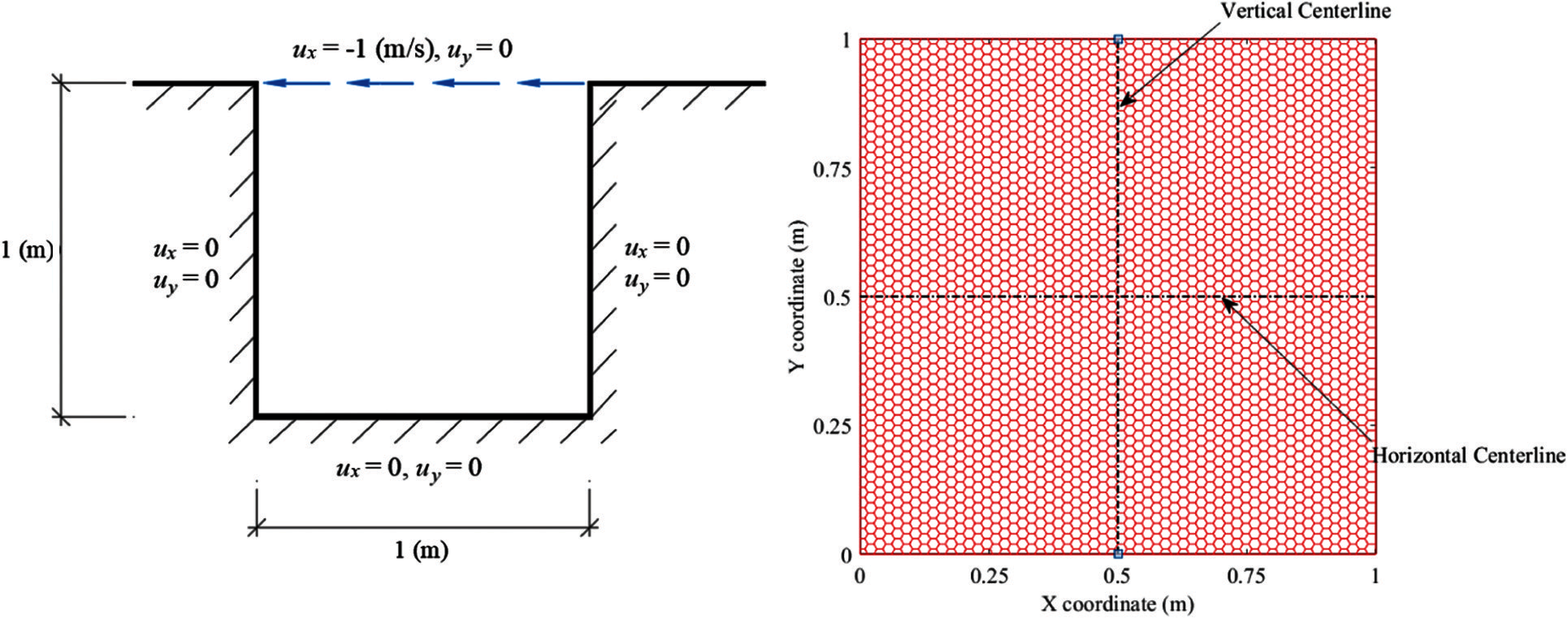
Figure 1: Left-lid-driven Cavity Domain; Right-A sample of hexagonal mesh

The initial results of this paper are presented in Fig. 2, indicating the velocity contours at the different Re of the cavity problem. As the initial observation, at the higher Re the positive contour centre of ux tend to reach to the bottom of the cavity. For the vertical velocity, the tendency is that the centres try to get lower and closer to the cavity walls. The next focus is the generation of the secondary contours at the cavity corners of simulations at the high Re, i.e., 1000, see Fig. 2. As fluid viscosity reduces, there is less resistance to fluid movement, which may explain those tendencies. Alternatively, as Re increases, the convection term becomes more prominent, resulting in more contour vortexes (see Eq. (42)).

For more profound validation, the velocities components (i.e., ux and uy) on the cavity centrelines (i.e., xc-vertical centreline and yc-horizontal one, respectively) are compared to the relevant literature, see Fig. 3. As seen in the figure, the entire agreement of our results to those of other studies, such as Ghia et al. [16], Botella et al. [14], Bruneau et al. [17], Erturk et al. [15], is apparent. For further details, see Tab. 1 of velocity values at reference points on the cavity centrelines, affirming our proposed method’s excellent performance. Like the table, the result of our proposed technique is very comparable to those seen in the literature, especially Ghia et al. [16]. For instance, the velocities at the domain’s centre point (0.5, 0.5) vary only by 1%–4% from the literature. Thus, an excellent or even marginally improved solution is provided. Following that, the extrema velocities on the centrelines are compared (see Fig. 4). Our recent results clearly mirrored those of Ghia et al. [16], Bottela et al. [14], Vanka [36] as well as Bruneau et al. [38].

Tab. 2 contains more information about the apparent proof for the convergence and precision of the new approach in this study. Moreover, our models computed on increasingly finer meshes steadily exceed the reference and convergence solution, as seen in Fig. 4 and Tab. 2. Furthermore, readers will see that our new results are greater than Ghia et al. [16] and Vanka [36], i.e., the results of uymin and uxmax, respectively.

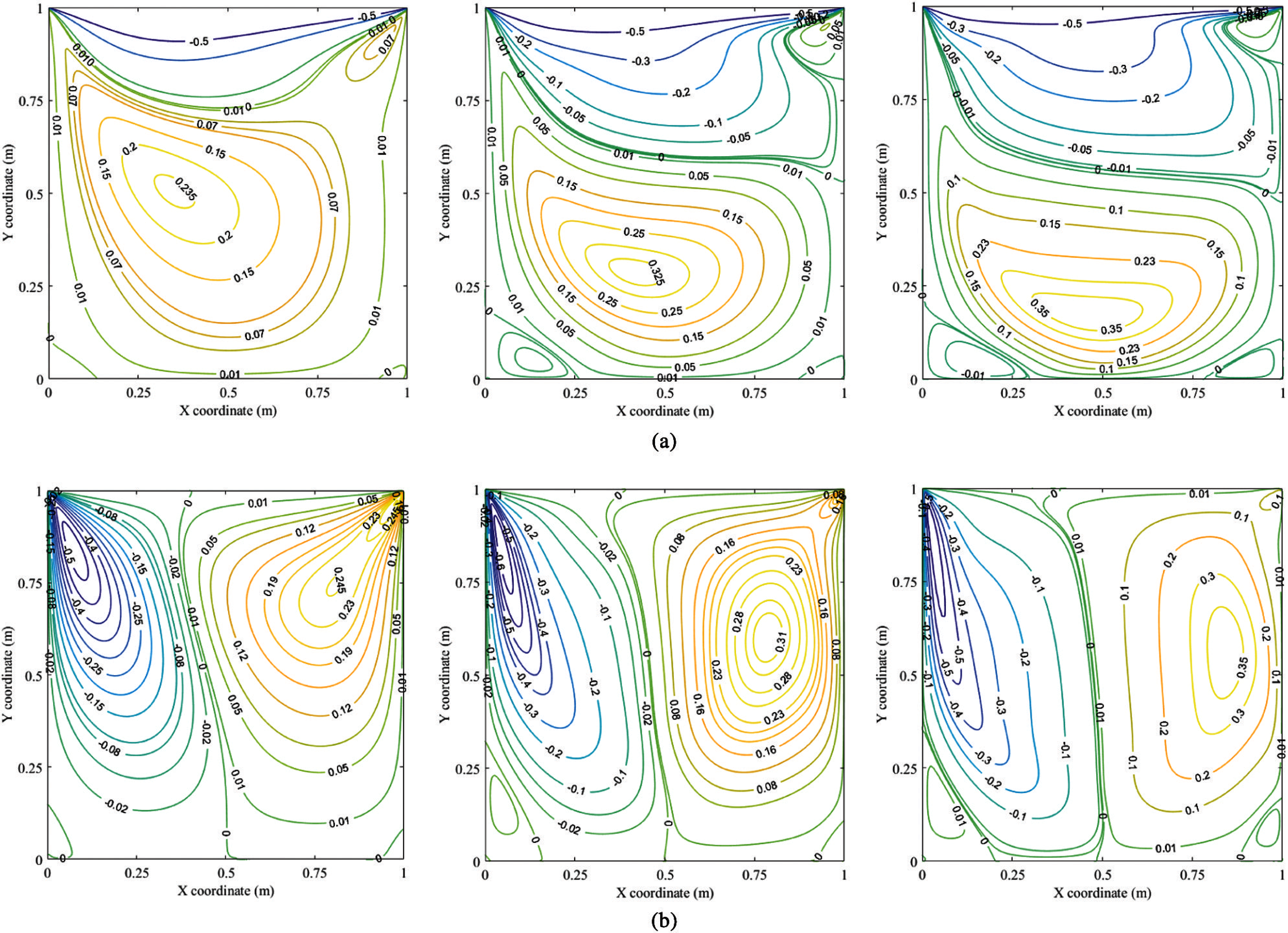
Figure 2: Contours of velocity fields (Left–Re=100; Middle - Re=400; Right–Re=1000). (a) Horizontal velocity field, ux. (b) Vertical velocity field, uy

The subsequent validation provided in this research is the results of fluid pressure. These results are firstly presented in Figs. 5 and 6 In which, Fig. 5 depicts the fluid pressures on the entire cavity using contour plots. These results indicate that as Re rises, the pressure primary contour's centre moves closer to the centre of cavity. As seen in Fig. 5, the rise also causes more secondary pressure contours to surround primary ones. Besides, the singularity of pressure at the cavity's top corners (0, 1) and (1, 1) is noteworthy. It occurs as a function of the abrupt change in velocity at those corners. References [40,41] explains this rule in terms of saddle-point theory.

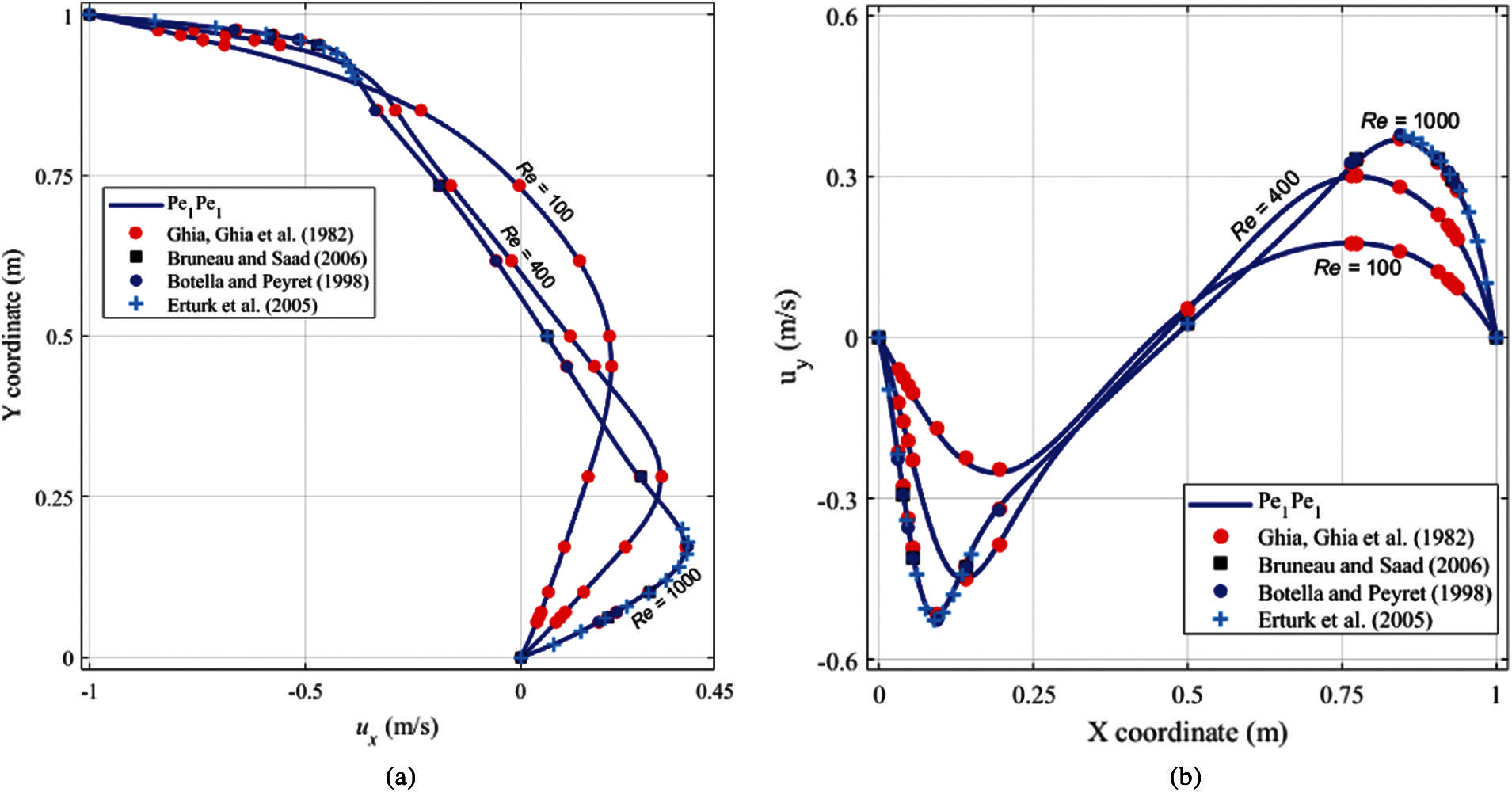
Figure 3: Velocity on the cavity centerlines. (a) ux–vertical velocity. (b) uy–horizontal velocity

The indications of pressure on the cavity centrelines are then seen in Fig. 6 to allow a detailed comparison with the literature. As the figure, it is evident that the current pressure results, i.e., the pressure at Re=1000 is completely close to the reference solution, i.e., Bottela et al. [14], Bruneau et al. [17]. Tab. 3 reveals seventeen points of pressure on the cavity centrelines for a more detailed comparison. The pressure results on several different progressively finer meshes are given in this table to show that our proposed solution is convergent. The results in the table convince the comparatively strong convergence of our recent method. It can be seen that our pressure results give an excellent fitting to the reference results in [14,17] (the disparity is about 3.7%). As known, the error of the other methods, for example, FDM to [16], typically is 4% [14]. Hence, it can be confirmed that our recent polygonal method provided an excellent solution for both velocity and pressure. It is crucial evidence of the new technique's performance in solving 2D incompressible steady N-S problems. The only concern is that there is not enough comparison data for pressures at other Re, such as 100 and 400, resulting in poor validity. However, it makes a significant contribution in terms of providing further reference data for future research. In other words, this study adds to the body of knowledge about fluid pressure by using previously unpublished evidence, such as the pressure of a lid-driven cavity flow at Re = 100 and 400, as in Tab. 3.

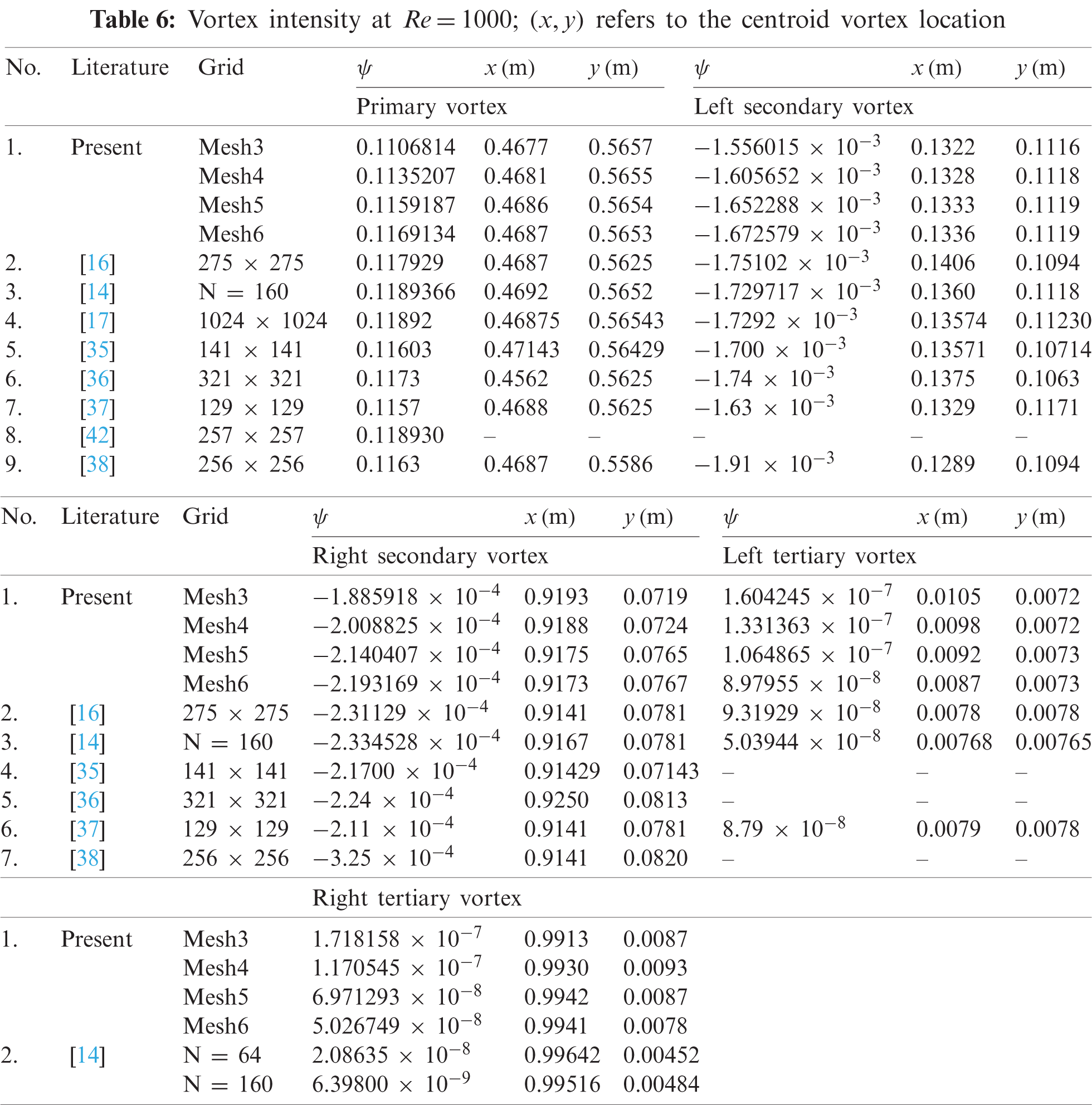
All the above results already exhibited a perfect convergence as well as the precision of velocity and pressure. Thus, the remaining part is to illustrate another result of streamlines. The first streamlines regarding the lid-driven cavity flow at Re = 100 are seen in Fig. 7a. As can be seen from this figure, the current streamlines are identical to Ghia et al. [16]. Furthermore, Figs. 7b and 7c provide a more in-depth analysis of the streamline effects by displaying all of the vortex centre properties (i.e., location, intensity). Besides, Tab. 4 displays the values of such data. It is concrete proof for this validation. In terms of the figure and table, it is easy to firm that the streamlines result completely match [16,35–38]. In addition, the convergence of the streamlines is also verified (see Tab. 4).

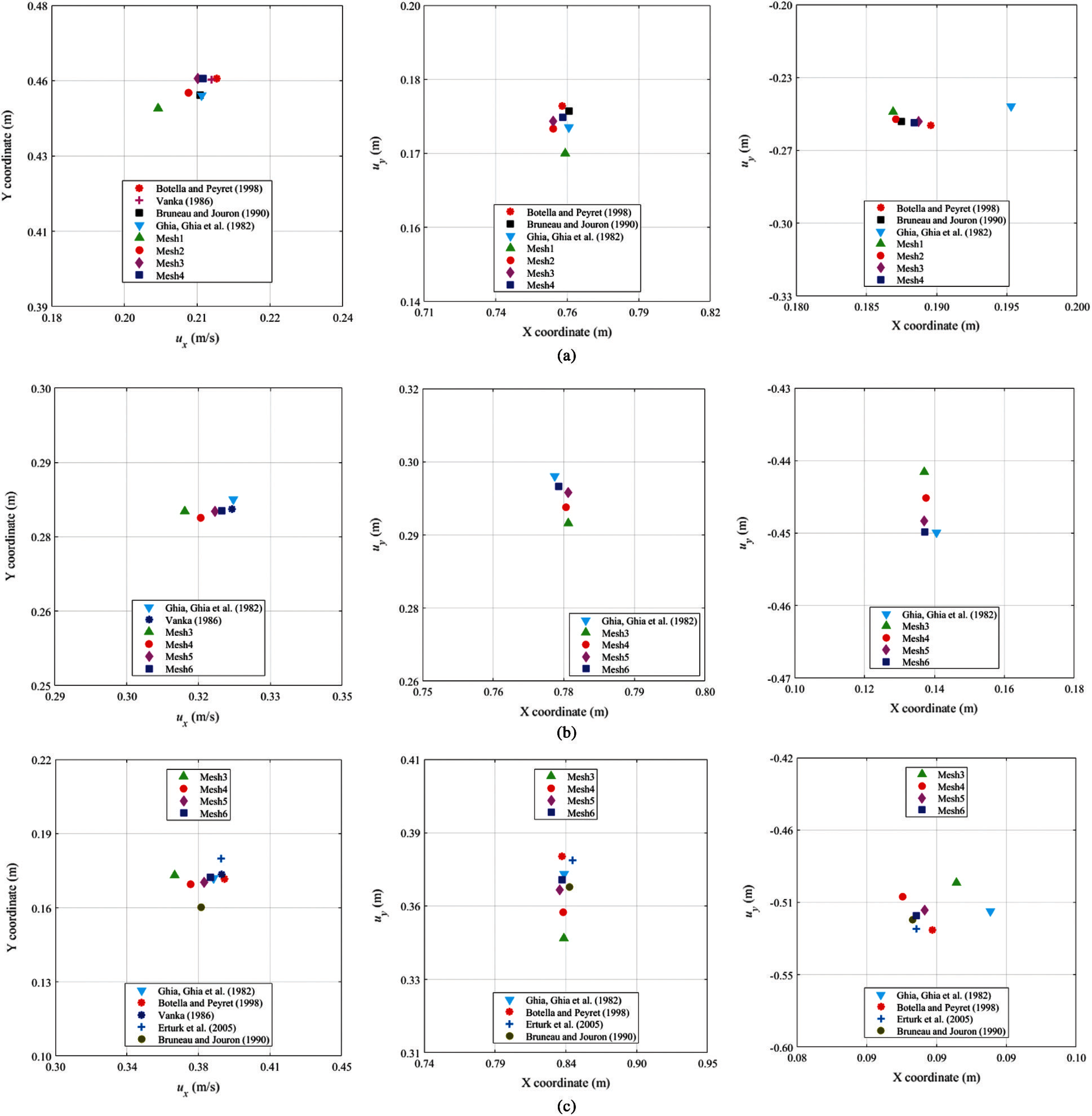
Figure 4: Locations of extrema velocities on the cavity centerlines (left-uxmax (m/s); middle-uymax and right-uymin) (a) Re=100 (b) Re=400 (c) Re=1000

Besides, the streamlined results of the lid-driven cavity simulation at Re = 400 are the subject of the following evaluation. They are illustrated in Fig. 8 and Tab. 5. They validate our recent results’ great matches to [16,35,36,42], as well as the enhanced polygonal method's good convergence and accuracy. The formation of another secondary vortex in the cavity’s right bottom corner, as seen in Fig. 8, is then of particular interest. As known, the flow at the bottom corners of the cavity is almost fragile (close to zero). The generation of secondary vortexes is supported by reduced friction force as the Reynolds number (viscosity) increases. It also explains the appearance of the tertiary vortices of the following simulation at Re=1000 (see Fig. 9). They are incredibly close to the bottom corners of the cavity where the intensity of vortices is entirely trivial (extremely close to zero, see Tab. 6). The intensities of left and right tertiary vortex, in particular, approximate 8.9×10−8 and 5.02×10−8, respectively. The accuracy of our current results is also identified in Fig. 9, which shows the closeness of the current vortex centres to the reference ones. Tab. 6 then indicates how the intensities and positions of vortex centres are close to those in [14,16,17,35–38].

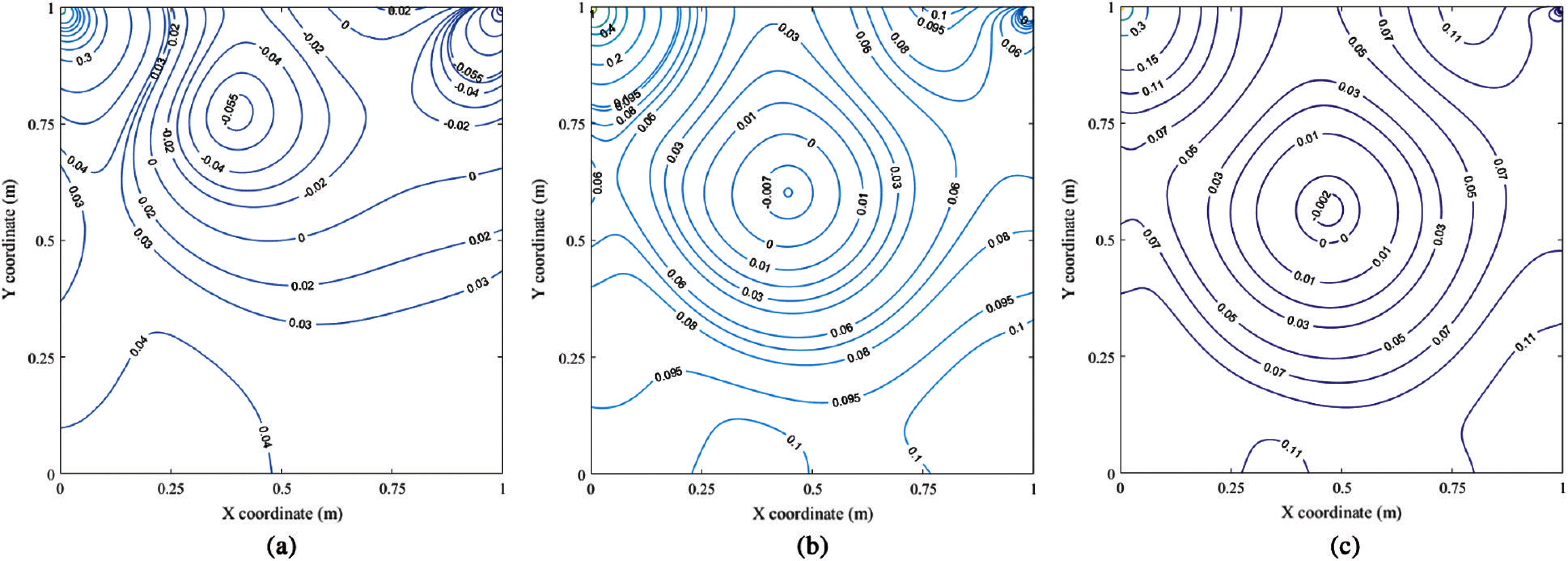
Figure 5: Fluid pressure contours (a) Re=100. (b) Re=400. (c) Re=1000.

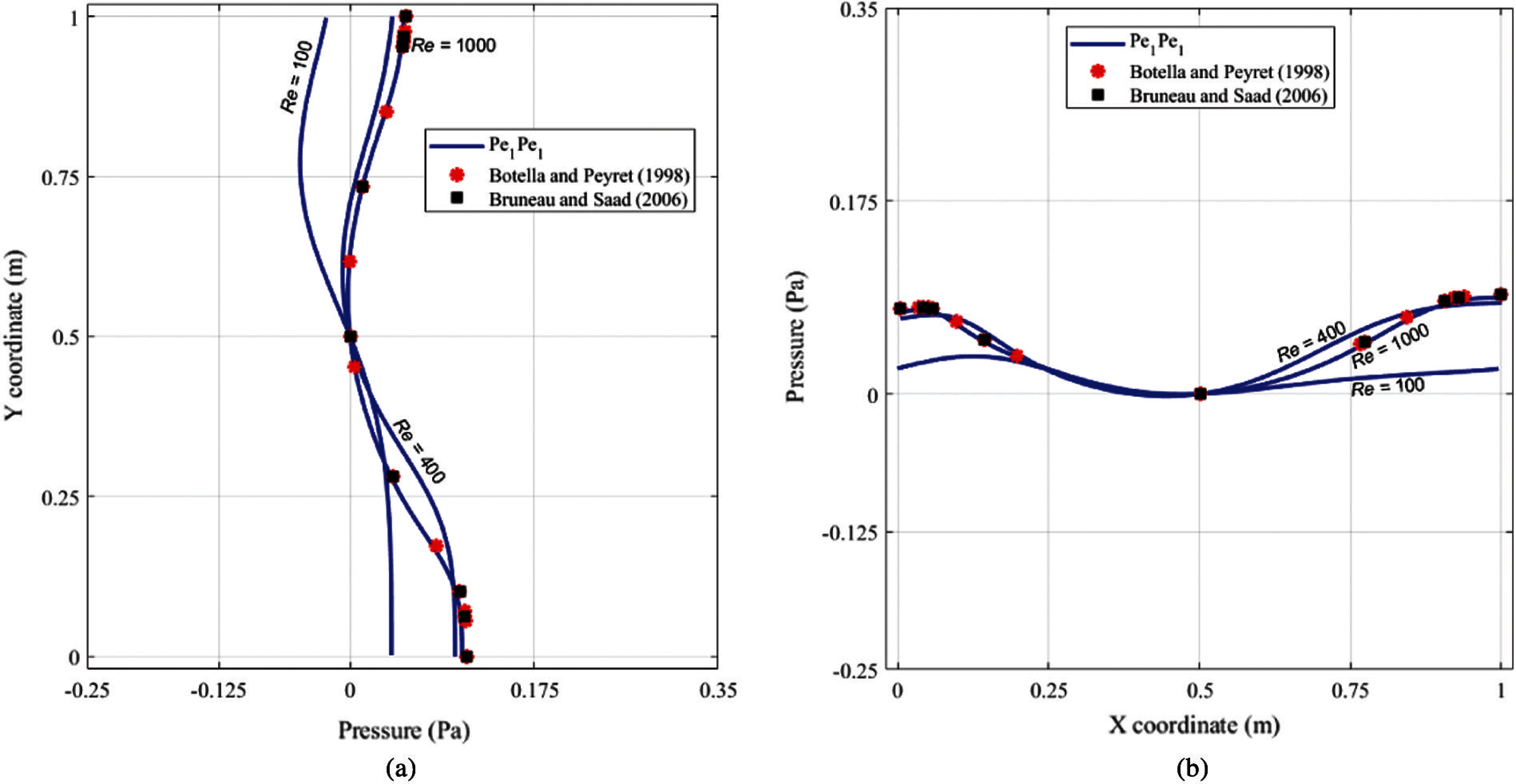
Figure 6: Fluid pressure on cavity centrelines. (a) Fluid pressure on the vertical centerline. (b) Fluid pressure on the horizontal centerline

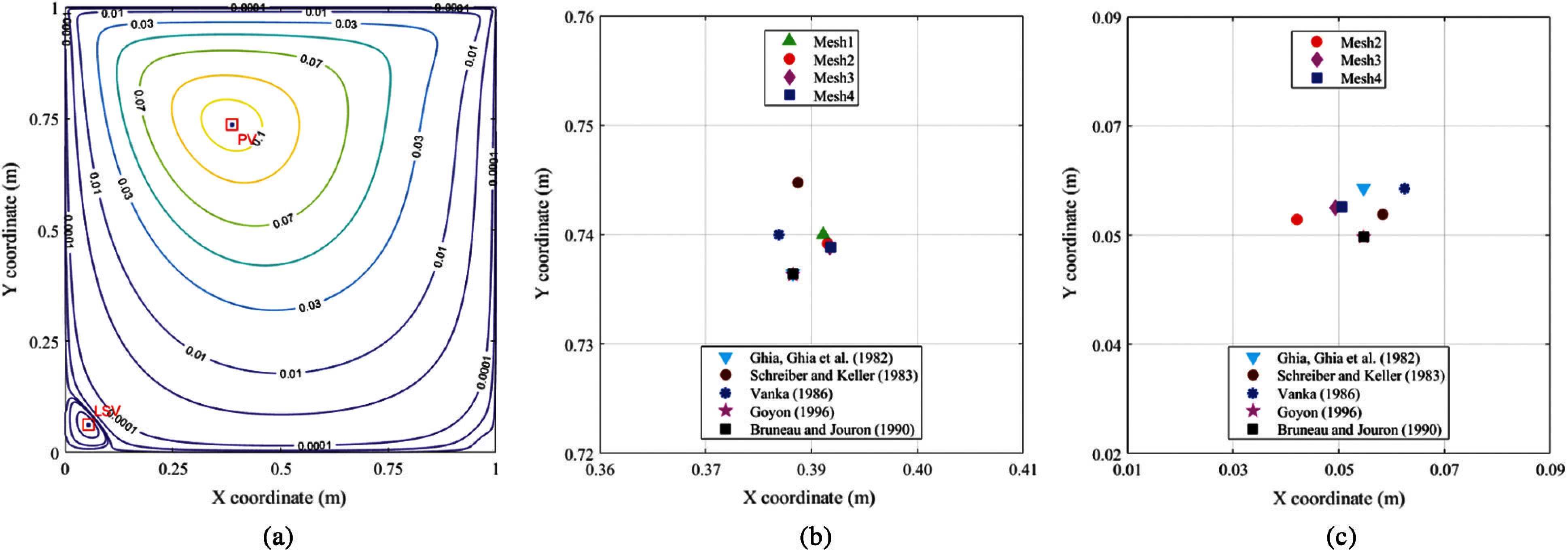
Figure 7: Streamline results of the cavity flow at Re=100. (a) Streamlines of the cavity flow. (b) Centre locations of the primary vortex (PV). (c) Centre locations of the left secondary vortex (LSV)

In conclusion, all the above results reveal that the present polygonal method is entirely good enough to deal with the 2D incompressible steady flows of lid-driven cavity benchmark. It is reinforced by numerous extensive comparisons to previously published research that used various highly precise techniques. For example, Botella et al. [14] in 1998 used the highly accurate Chebyshev collocation method associated with the subtraction method of the leading terms of the asymptotic expansion to obtain a highly accurate spectral solution with a maximum of grid mesh of N=160 (polynomial degree). Erturk et al. [15] 2005 applied FDM and spectral method to provide a high spatial accuracy solution of driven cavity flow. Bruneau et al. [17] in 2006 utilised the finite difference discretisation and the multigrid solver with a cell-by-cell relaxation procedure.

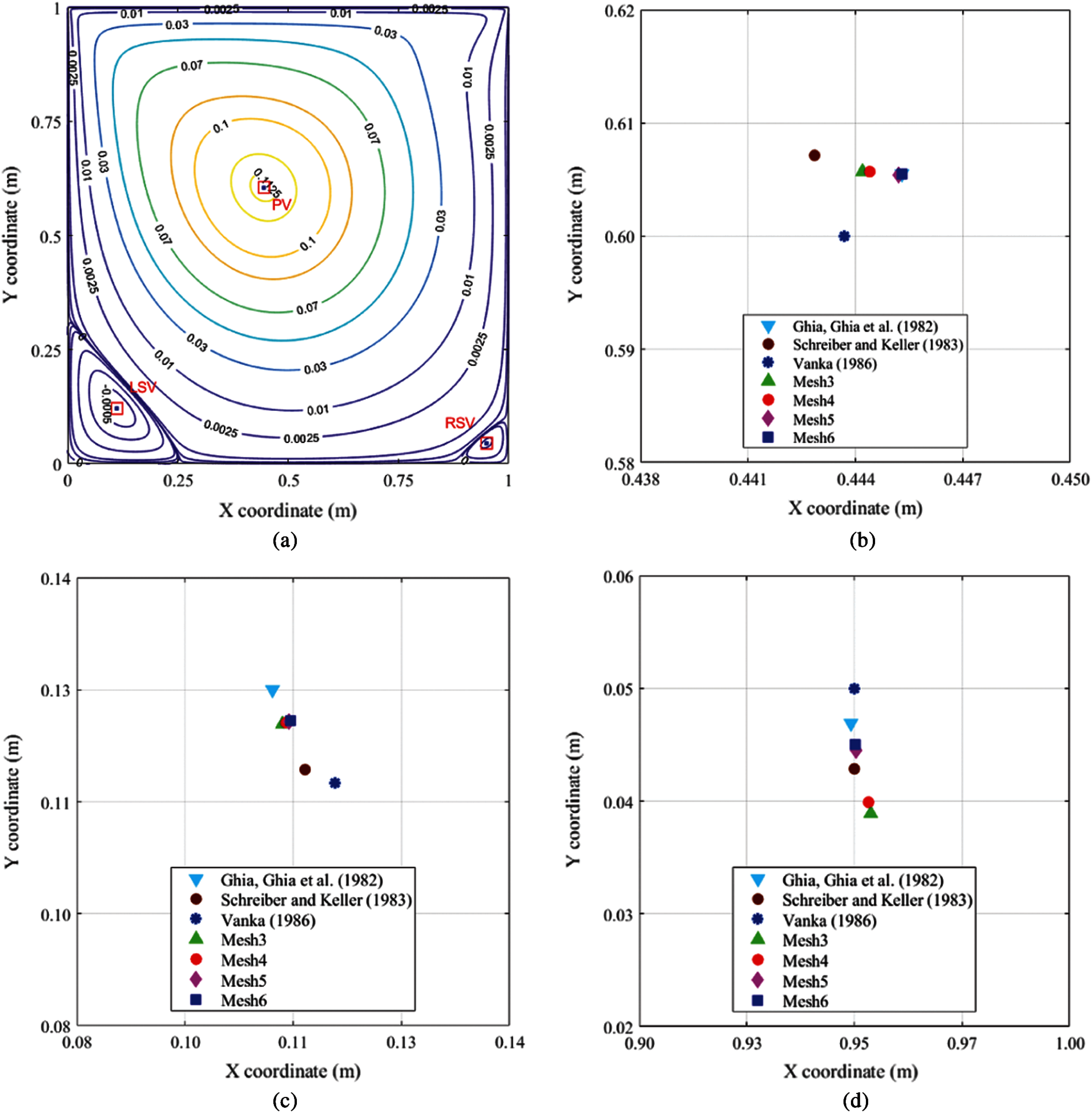
Figure 8: Streamline results of the cavity flow at Re=400. (a) Streamlines of the cavity flow. (b) Centre locations of the primary vortex (PV). (c) Centre locations of the left secondary vortex (LSV). (d) Centre locations of the right secondary vortex (RSV)

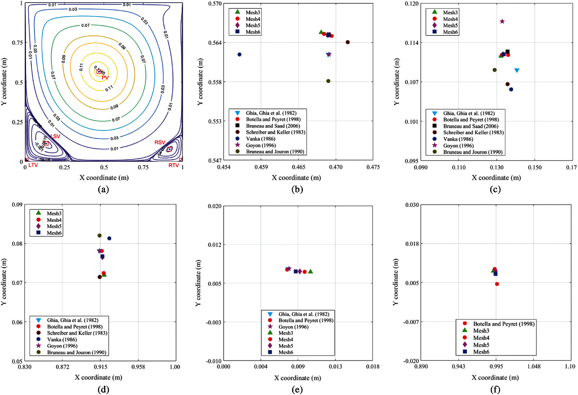
Figure 9: Streamline results of the cavity flow at Re=1000. (a) Streamlines of the cavity flow. (b) Centre locations of PV. (c) Centre locations of LSV. (d) Centre locations of the right secondary vortex (RSV). (e) Centre locations of the left tertiary vortex (LTV). (f) Centre locations of the right tertiary vortex (RTV)

6  Conclusion

To summarise, this research’s commitment to designing new PFEM to solve 2D incompressible steady fluid flows controlled by N-S equations is practical. This contribution is focused on the development of a mixed-order equal-order system. This idea then applies Wachspress basis shape functions associated with our advanced stabilisation technique to generate the equal-order mixed PFE, called Pe1Pe1 [10]. Furthermore, in this article, we successfully address the Picard iteration technique for our proposed PFE to deal with the nonlinear convection term of N-S equations. This paper incorporates a widely mathematical benchmark to evaluate the accuracy and performance of our developed PFE. It is the lid-driven cavity benchmark executed to measure the efficiency of numerical methods in solving N-S problems. Our established method shows an excellent agreement with the highly accurate solutions found in the literature regarding current research solutions. It means that the efficacy of our proposed technique for solving incompressible steady N-S fluid flows has been proven without any reasonable doubt.

Furthermore, the production of higher-order PFEs is a high-potential direction for future research in this field. For example, Rand et al. [43] suggest a novel quadratic serendipity shape function in 2014, a solid foundation for this direction. Alternatively, the Taylor–Hood elements, as described in [44], could be a good start. Additionally, extending our proposed PFEs to computations for transient fluid flow problems is a significant strategic work of this study. The proposed method's application to 3D problems is, therefore, a priority task. Other promising ideas for future research are free surface and fluid-structure interaction problems. In addition, in recent years, Deep Neural Networks (DNNs) developments are becoming a mathematical option to solve the partial differential equations (PDEs) of different phenomena in science and engineering [45,46]. Thus, the efficiency of DNNs is an exciting direction for this research.

Funding Statement: This work was supported by the VLIR-UOS TEAM Project, VN2017TEA454A 103, ‘An innovative solution to protect Vietnamese coastal riverbanks from floods and erosion’ funded by the Flemish Government.

Conflicts of Interest: The authors declare that they have no conflicts of interest to report regarding the present study.

References

 1.  T. Narasimhan and P. Witherspoon, “An integrated finite difference method for analyzing fluid flow in porous media,” Water Resources Research, vol. 12, no. 1, pp. 57–64, 1976. [Google Scholar]

 2.  M. A. Sayed, H. A. Kandil and A. Shaltot, “Aerodynamic analysis of different wind-turbine-blade profiles using finite-volume method,” Energy Conversion and Management, vol. 64, no. 2, pp. 541–550, 2012. [Google Scholar]

 3.  O. C. Zienkiewicz, R. L. Taylor and J. Zhu, Finite Element Method: Its Basis and Fundamentals, 7th ed., Oxford: Butterworth-Heinemann, 2013. [Google Scholar]

 4.  D. Sieger, P. Alliez and M. Botsch, “Optimizing voronoi diagrams for polygonal finite element computations,” in Proc. of the 19th Int. Meshing Roundtable, Chattanooga, Tennessee, USA, pp. 335–350, 2010. [Google Scholar]

 5.  C. Talischi, G. H. Paulino, A. Pereira and I. F. Menezes, “PolyMesher: A general-purpose mesh generator for polygonal elements written in Matlab,” Structural and Multidisciplinary Optimization, vol. 45, no. 3, pp. 309–328, 2012. [Google Scholar]

 6.  C. Talischi, A. Pereira, G. H. Paulino, I. F. Menezes and M. S. Carvalho, “Polygonal finite elements for incompressible fluid flow,” International Journal for Numerical Methods in Fluids, vol. 74, no. 2, pp. 134–151, 2014. [Google Scholar]

 7.  K. N. Chau, K. N. Chau, T. Ngo, K. Hackl and H. Nguyen-Xuan, “A polytree-based adaptive polygonal finite element method for multi-material topology optimization,” Computer Methods in Applied Mechanics and Engineering, vol. 332, no. 2, pp. 712–739, 2018. [Google Scholar]

 8.  H. Chi, C. Talischi, O. Lopez-Pamies and G. H. Paulino, “Polygonal finite elements for finite elasticity,” International Journal for Numerical Methods in Engineering, vol. 101, no. 4, pp. 305–328, 2015. [Google Scholar]

 9.  T. Vu-Huu, C. Le-Thanh, H. Nguyen-Xuan and M. Abdel-Wahab, “A high-order mixed polygonal finite element for incompressible Stokes flow analysis,” Computer Methods in Applied Mechanics and Engineering, vol. 356, pp. 175–198, 2019. [Google Scholar]

10. T. Vu-Huu, C. Le-Thanh, H. Nguyen-Xuan and M. Abdel-Wahab, “An equal-order mixed polygonal finite element for two-dimensional incompressible Stokes flows,” European Journal of Mechanics-B/Fluids, vol. 79, pp. 92–108, 2020. [Google Scholar]

11. H. T. Vu, T. C. Le, H. Nguyen-Xuan and M. Abdel Wahab, “Stabilization for equal-order polygonal finite element method for high fluid velocity and pressure gradient,” Computers, Materials & Continua, vol. 62, no. 3, pp. 1109–1123, 2020. [Google Scholar]

12. T. Vu-Huu, C. Le-Thanh, H. Nguyen-Xuan and M. A. Wahab, “Equal-order polygonal analysis for fluid computation in curved domain,” International Journal of Computational Methods, vol. 18, no. 5, pp. 2040003, 2020. [Google Scholar]

13. C. R. Dohrmann and P. B. Bochev, “A stabilized finite element method for the Stokes problem based on polynomial pressure projections,” International Journal for Numerical Methods in Fluids, vol. 46, no. 2, pp. 183–201, 2004. [Google Scholar]

14. O. Botella and R. Peyret, “Benchmark spectral results on the lid-driven cavity flow,” Computers & Fluids, vol. 27, no. 4, pp. 421–433, 1998. [Google Scholar]

15. E. Erturk, T. C. Corke and C. Gökçöl, “Numerical solutions of 2-D steady incompressible driven cavity flow at high Reynolds numbers,” International Journal for Numerical Methods in Fluids, vol. 48, no. 7, pp. 747–774, 2005. [Google Scholar]

16. U. Ghia, K. N. Ghia and C. Shin, “High-Re solutions for incompressible flow using the Navier–Stokes equations and a multigrid method,” Journal of Computational Physics, vol. 48, no. 3, pp. 387–411, 1982. [Google Scholar]

17. C.-H. Bruneau and M. Saad, “The 2D lid-driven cavity problem revisited,” Computers & Fluids, vol. 35, no. 3, pp. 326–348, 2006. [Google Scholar]

18. H. T. Vu, “Polygonal finite element methods to analyse incompressible steady fluid flows,” Ph.D. dissertation. Ghent University, Belgium, 2020. [Google Scholar]

19. C. T. Kelley, Iterative Methods for Linear and Nonlinear Equations, Philadelphia: Society for Industrial and Applied Mathematics, 1995. [Google Scholar]

20. I. A. Abbas and H. M. Youssef, “A nonlinear generalized thermoelasticity model of temperature-dependent materials using finite element method,” International Journal of Thermophysics, vol. 33, no. 7, pp. 1302–1313, 2012. [Google Scholar]

21. L. Esch, R. Kieffer and T. Lopez, Asset and Risk Management: Risk Oriented Finance. Hoboken, New Jersey: John Wiley & Sons, 2005. [Google Scholar]

22. G. Palani and I. Abbas, “Free convection MHD flow with thermal radiation from an impulsively-started vertical plate, Nonlinear Analysis,” Modelling and Control, vol. 14, no. 1, pp. 73–84, 2009. [Google Scholar]

23. O. A. Karakashian, “On a Galerkin–Lagrange multiplier method for the stationary Navier–Stokes equations,” SIAM Journal on Numerical Analysis, vol. 19, no. 5, pp. 909–923, 1982. [Google Scholar]

24. H.-G. Roos, M. Stynes and L. Tobiska, Robust Numerical Methods for Singularly Perturbed Differential Equations: Convection-Diffusion-reaction and Flow Problems. Berlin, Springer: Springer Science & Business Media, 2008. [Google Scholar]

25. H. C. Elman, D. J. Silvester and A. J. Wathen, Finite Elements and Fast Iterative Solvers: With Applications in Incompressible Fluid Dynamics. UK: Oxford University Press, 2014. [Google Scholar]

26. M. A. Celia, E. T. Bouloutas and R. L. Zarba, “A general mass-conservative numerical solution for the unsaturated flow equation,” Water Resources Research, vol. 26, no. 7, pp. 1483–1496, 1990. [Google Scholar]

27. M. Floater, A. Gillette and N. Sukumar, “Gradient bounds for Wachspress coordinates on polytopes,” SIAM Journal on Numerical Analysis, vol. 52, no. 1, pp. 515–532, 2014. [Google Scholar]

28. E. L. Wachspress, “Barycentric coordinates for polytopes,” Computers & Mathematics with Applications, vol. 61, no. 11, pp. 3319–3321, 2011. [Google Scholar]

29. H. Nguyen-Xuan, S. Nguyen-Hoang, T. Rabczuk and K. Hackl, “A polytree-based adaptive approach to limit analysis of cracked structures,” Computer Methods in Applied Mechanics and Engineering, vol. 313, no. 5, pp. 1006–1039, 2017. [Google Scholar]

30. Y. Nakayama, Introduction to Fluid Mechanics. Oxford, UK: Butterworth-Heinemann, 2018. [Google Scholar]

31. D. F. Young, B. R. Munson, T. H. Okiishi and W. W. Huebsch, A Brief Introduction to Fluid Mechanics. Hoboken, New Jersey: John Wiley & Sons, 2010. [Google Scholar]

32. T. Vu-Huu, P. Phung-Van, H. Nguyen-Xuan and M. A. Wahab, “A polytree-based adaptive polygonal finite element method for topology optimization of fluid-submerged breakwater interaction,” Computers & Mathematics with Applications, vol. 76, no. 5, pp. 1198–1218, 2018. [Google Scholar]

33. V. Girault and P.-A. Raviart, Finite Element Methods for Navier–Stokes Equations: Theory and Algorithms. Berlin, Germany: Springer Science & Business Media, 2012. [Google Scholar]

34. R. Rannacher, Finite Element Methods for the Incompressible Navier–Stokes Equations. Berlin, Germany: Springer, 2000. [Google Scholar]

35. R. Schreiber and H. B. Keller, “Driven cavity flows by efficient numerical techniques,” Journal of Computational Physics, vol. 49, no. 2, pp. 310–333, 1983. [Google Scholar]

36. S. P. Vanka, “Block-implicit multigrid solution of Navier–Stokes equations in primitive variables,” Journal of Computational Physics, vol. 65, no. 1, pp. 138–158, 1986. [Google Scholar]

37. O. Goyon, “High-Reynolds number solutions of Navier–Stokes equations using incremental unknowns,” Computer Methods in Applied Mechanics and Engineering, vol. 130, no. 3–4, pp. 319–335, 1996. [Google Scholar]

38. C.-H. Bruneau and C. Jouron, “An efficient scheme for solving steady incompressible Navier–Stokes equations,” Journal of Computational Physics, vol. 89, no. 2, pp. 389–413, 1990. [Google Scholar]

39. G. Deng, J. Piquet, P. Queutey and M. Visonneau, “Incompressible flow calculations with a consistent physical interpolation finite volume approach,” Computers & Fluids, vol. 23, no. 8, pp. 1029–1047, 1994. [Google Scholar]

40. F. Brezzi and M. Fortin, “Incompressible materials and flow problems,” in Mixed and Hybrid Finite Element Methods, New York, NY: Springer, pp. 200–273, 1991. [Google Scholar]

41. T. Rusten and R. Winther, “A preconditioned iterative method for saddlepoint problems,” SIAM Journal on Matrix Analysis and Applications, vol. 13, no. 3, pp. 887–904, 1992. [Google Scholar]

42. E. Barragy and G. Carey, “Stream function-vorticity driven cavity solution using p finite elements,” Computers & Fluids, vol. 26, no. 5, pp. 453–468, 1997. [Google Scholar]

43. A. Rand, A. Gillette and C. Bajaj, “Quadratic serendipity finite elements on polygons using generalized barycentric coordinates,” Mathematics of Computation, vol. 83, no. 290, pp. 2691–2716, 2014. [Google Scholar]

44. C. Taylor and P. Hood, “A numerical solution of the Navier–Stokes equations using the finite element technique,” Computers & Fluids, vol. 1, no. 1, pp. 73–100, 1973. [Google Scholar]

45. E. Samaniego, C. Anitescu, S. Goswami, V. M. Nguyen-Thanh, H. Guo et al., “An energy approach to the solution of partial differential equations in computational mechanics via machine learning: Concepts, implementation and applications,” Computer Methods in Applied Mechanics and Engineering, vol. 362, no. 2, pp. 112790, 2020. [Google Scholar]

46. C. Anitescu, E. Atroshchenko, N. Alajlan and T. Rabczuk, “Artificial neural network methods for the solution of second order boundary value problems,” Computers, Materials and Continua, vol. 59, no. 1, pp. 345–359, 2019. [Google Scholar]

Appendix A.

This work is licensed under a Creative Commons Attribution 4.0 International License, which permits unrestricted use, distribution, and reproduction in any medium, provided the original work is properly cited.