DOI:10.32604/cmc.2022.020926
| Computers, Materials & Continua DOI:10.32604/cmc.2022.020926 | |
| Article |
Hybrid Sensor Selection Technique for Lifetime Extension of Wireless Sensor Networks
1Information Systems Department, Faculty of Computers and Artificial Intelligence, Benha University, Benha, 13518, Egypt
2Faculty of Artificial Intelligence, Kafrelsheikh University, Kafrelsheikh, 33516, Egypt
3Electrical Engineering Department, Benha Faculty of Engineering, Benha University, Benha, 13518, Egypt
*Corresponding Author: Basma M. Hassan. Email: basma.mohamed@ai.kfs.edu.eg
Received: 14 June 2021; Accepted: 15 July 2021
Abstract: Energy conservation is a crucial issue to extend the lifetime of wireless sensor networks (WSNs) where the battery capacity and energy sources are very restricted. Intelligent energy-saving techniques can help designers overcome this issue by reducing the number of selected sensors that report environmental measurements by eliminating all replicated and unrelated features. This paper suggests a Hybrid Sensor Selection (HSS) technique that combines filter-wrapper method to acquire a rich-informational subset of sensors in a reasonable time. HSS aims to increase the lifetime of WSNs by using the optimal number of sensors. At the same time, HSS maintains the desired level of accuracy and manages sensor failures with the most suitable number of sensors without compromising the accuracy. The evaluation of the HSS technique has adopted four experiments by using four different datasets. These experiments show that HSS can extend the WSNs lifetime and increase the accuracy using a sufficient number of sensors without affecting the WSN functionality. Furthermore, to ensure HSS credibility and reliability, the proposed HSS technique has been compared to other corresponding methodologies and shows its superiority in energy conservation at premium accuracy measures.
Keywords: Energy conservation; WSNs; intelligent techniques; sensor selection
Wireless Sensor Networks (WSNs) could be described as a group of connected sensor nodes [1], which are small-sized devices with restricted resources such as power supply and memory. In a traditional sensor network, every node should monitor physical environmental prerequisites like sound, temperature, pressure, humidity, motion, light, vibration, etc. In a sensor network [2], sensors can co-operate to rise out a particular purpose because of the nature of the observed parameters and the enormous quantity of implemented sensors. The generated information from the sensor network is quite correlated, and reporting every individual sensor reading is a waste of energy resources. Besides, many motives had highlighted the significance of machine learning methodologies’ adoption in WSNs applications to learn about and discover correlated data, predictions, decisions, and information or data classification. The first reason is that sensor nodes aren't operating as predicted due to sudden environmental behavior. The second reason is because of the unpredictable environments where WSNs are distributed.
The third reason is that sensor nodes produce massive quantities of correlated and replicated data. The energy-efficient conservation scheme was illustrated [3] to prolong the network lifetime. A lot of energy in sensor nodes is wasted in data communication. Hence, decreasing the quantity of unnecessary communication helped minimize energy waste and extended the overall network lifespan. Furthermore, designing a high-quality strength management scheme is one of the principal challenges of WSNs. Many research efforts have been spent using intelligent techniques based totally on machine learning. It has been efficiently utilized for various scientific purposes, specifically with linear kernel, which can analyze and construct the required information from fewer training samples, nevertheless offers excessive classification accuracy. The classification algorithms, such as K-Nearest Neighbor (K-NN) [4], Support Vector Machine (SVM) [5], and Random Forest (RF) [6], are adopted extensively and investigated in the region of machine learning. SVM is additionally regarded as a too effective algorithm in the subject of data-mining [7].
The problem statement stems from energy in WSNs which is a rare commodity, particularly in cases wherever it would be hard to supply additional energy sources if the available energy were used up. Even in scenarios where energy harvesting is possible, efficient energy usage remains a crucial objective to extend the life of the network. Therefore, the main goal in designing WSNs are to keep the energy consumption of sensors as low as possible since the main issue is the limited battery capacity of sensors. The major objective of the above methods is to raise the network performance by eliminating noisy, redundant, and irrelevant features. In this paper, the number of features is reduced to limit the energy consumption of sensors. Therefore, extending the lifetime of the network, while maintaining a certain level of classification accuracy.
The paper assumes that sensors in a wireless network are only activated on demand from the base station (sink node) of the underlying system (platform). Moreover, each sensor measures one feature from the environment and returns its value to the base station, where the proposed HSS is executed. Hence, classifier training and validation are executed on the base station as well because the ML techniques will increase energy consumption if they are implemented separately in each node of the network.
The paper contributions are summarized below:
• Provides detailed earlier energy efficiency methods related to working in WSNs based on intelligent ML models and algorithms.
• Suggest a Hybrid Sensor Selection (HSS) technique that minimizes the number of sensors to reduce the sensors’ energy consumption and increase the network's lifetime maintaining a proven phase of classification accuracy.
• This HSS technique combines the filter-wrapper method to acquire an informative subset of sensors in a reasonable time.
• Four dissimilar and extensive experiments were conducted to demonstrate the effectiveness of the proposed technique for improving the WSNs lifespan.
• The proposed HSS technique is compared with existing approaches on measurement tasks, datasets and its superiority is highlighted.
The rest of this paper is organized as follows. Section 2 reviews the state of the art in sensor selection and energy-efficient schemes based on intelligent models WSNs. The main contribution of this paper is presented in Section 3 through the HSS proposed technique. Section 4 discusses simulation experiments and setup. Simulation results are summarized in Section 5. Finally, Section 6 concludes the paper and highlights future research directions.
The following part of this survey will provide a literature review of recent approaches proposed for energy conservation for WSNs based on machine learning and intelligent energy-saving models and energy conservation through energy management has lengthy records or history.
Discriminative extracted features are used to enhance the computational efficiency of the suggested model using Naïve Bayes, multilayers perceptron (MLP), and SVM. The intelligent energy management models have been introduced to maximize WSNs lifetime and decrease the number of chosen sensors to environmental measurements achieving high energy-efficient network while keeping the preferred degree of accuracy in the mentioned readings. This selection approach has ranked sensors based on the importance of their usage, from the best to the least important using three intelligent models based on Naïve Bayes, MLP, and SVM classifiers. The MATLAB simulation outcomes showed that Linear SVM chosen sensors produced higher energy efficiency than those chosen through Naïve Bayes and MLP for equal Lifetime Extension Factor (LEF) of WSNs [8].
Other associated research work offered a massive range of selection criteria to handle characteristic importance, like Laplacian score and Fisher rating [9]. These techniques addressed several combinatorial optimization bottlenecks, such as local optimality and costly computational value. A hybrid methodology was proposed [10] based on wavelet transform (WT) and mutual information change (MIC) for faulty sensor identification. The results showed that approaches WT and MIC obtained a more considerable accuracy in most fault varieties. Another hybrid model was proposed [11] using Rough Set Theory (RST), Binary Grey Wolf Optimization Algorithm, and Chaos Theory for feature selection problems. Results indicated that the proposed method showed higher performance, more incredible speed, lower error, and shorter execution time.
The partly informed sparse auto encoder (PISAE) that primarily based energy conservation is brought in [12] for prolonging the WSNs lifetime. PISAE aimed to improve lifespan by inserting sensors with redundant readings to sleep without dropping big information. PISAE overall performance was tested on three specific datasets using MLP, Naïve Bayes, and SVM classifiers. The decision scheme was proposed [13] to minimize the strength consumption of WSNs. The sensors were sorted top-down from the most to the least based on the importance and usage in WSNs. Hence, the Naïve Bayes method has been used. The later stated method has been tested on many popular actual datasets. The results have shown that extra energy is fed on if excellent sensors are used, then the sensor network lifetime is minimized. The linear SVM [14] performed better compared to most of machine learning classifiers presented. More interest has been dedicated to this classifier for its outstanding performance in classification accuracy phrases. Therefore, this intelligent classifier has been utilized in a variety of applications. The energy management in WSNs was proposed [15] to reduce the number of specific sensors that report measurements. The results indicated that the multilayer perceptron MLP algorithm achieved a significant accuracy enhancement compared to Naïve Bayes during the same lifetime extension factor.
In [16] energy-saving framework for WSNs was proposed using machine learning techniques and meta-heuristics used two-phase energy savings on the sensor nodes. The first phase, network-level energy-saving, was achieved by finding the minimum sensor nodes needed. To find the minimum sensor nodes, they applied hybrid filter wrapper feature selection to find the best feature subsets and found the measures don't produce significant performance differences from 20%. In the second phase, they achieved energy savings of the WSNs by manipulating the sampling rate and the transmission interval of the sensor nodes to achieve node level energy saving. They proposed an optimization method based on Simulated Annealing (SA), but this approach reduced energy consumption by more than 90%. But, this work has some limitations such as it has a lack of scalability to handle changes in the WSNs and the second limitation is due to bad routing protocols and complex topology their approach may be infeasible in the real world.
The intelligent technique for energy-efficient conservation in WSNs is introduced using classification methodologies. In this paper, Sensor Discrimination, Ionosphere, ISOLET, and Forest Cover Type datasets have been used to challenge the superiority of the intelligent algorithms in phrases of classification accuracy and the Lifetime Extension Factor (LEF) that is shown in Eq. (1).
The lifetime extension factor is the ratio between the total number of network sensors and the number of sensors used by HSS for a specific experiment:
Understandably, LEF minimum value is limited to 1, which reflects that the network administrator always uses all sensors in each classification step, which should reveal the highest possible accuracy measure. Contrarily, if fewer sensors are selected/used for that specific network, the value of LEF will be greater than 1; as a result the network lifespan will be extended. In addition, one of the research assumptions is that each sensor can be used properly M times before it goes unavailable, which also reflects the sensor lifetime based on its energy consumed in measurement and network connectivity. The key point here is to save sensor/network energy for irrelevant or redundant sensors. That reveals that, LEF is inversely proportional to the network energy consumption. The higher the LEF value the lower the network energy consumption. If HSS could increase the LEF then the energy conservation of the network will be achieved, while maintaining network functionality and accuracy within the accepted constraints.
The main purpose of HSS is to choose the most suitable number of features (sensors) in the preprocessing stage based on hybrid statistical (filter-wrapper) methods and examine the proposed technique superiority using the classification accuracy. Two necessary steps are carried out to conserve the energy and prolong the lifetime factor of sensor nodes. First, the most dominant sensor nodes in WSNs had been chosen based on the proposed Hybrid Sensor Selection (HSS) technique. Second, the K-NN, Linear-SVM, and RF classification algorithms are applied for efficient energy conservation in WSNs and delivered through the classification algorithm's capability by means of using SVM. The proposed technique operates in four stages, as shown in Fig. 1.
In the preprocessing procedure, the first step is needed to obtain the related dataset. This dataset should consist of the data collected from several WSNs environment resources. Four datasets have been examined, which are obtained from the public UCI and Kaggle. In the pre-processing stage, as in Fig. 2, it is vital to identify and handle the missing records correctly. If not, that may pull inexact and wrong conclusions out of the data.
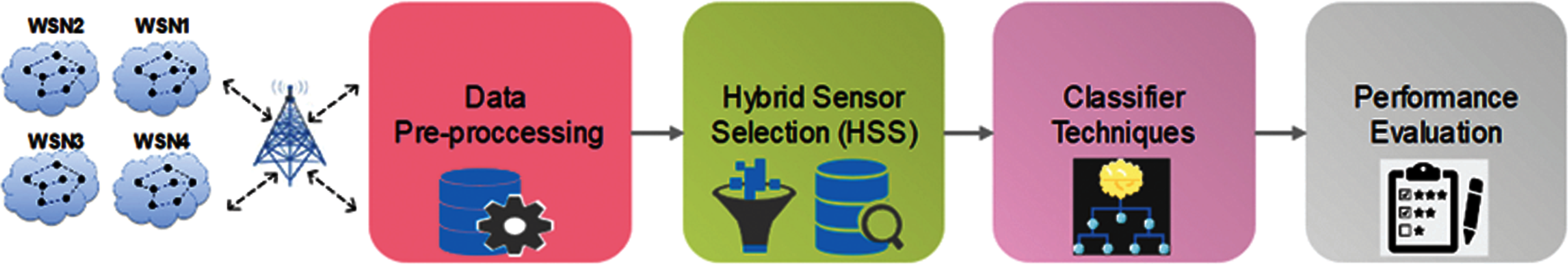
Figure 1: General architecture of the proposed technique

Figure 2: Data preprocessing
3.2 Hybrid Sensor Selection (HSS) Technique
The importance of the sensor selection in the proposed HSS technique comes from feature selection in the machine learning algorithm. This work uses the hybrid sensor selection that consists of filter methods and a wrapper method, as shown in Fig. 3. The datasets collected after preprocessing data are used as inputs to the HSS technique. The selection of sensors is independent of any machine learning algorithms. Instead, sensors are chosen based on their scores on different statistical tests to correlate with the outcome. This HSS technique consists of four steps to obtain a sub-optimal set of sensors. The first step is a blend of filter techniques that are carried out to reduce the number of sensors. Each filter technique calculates a score for every sensor.
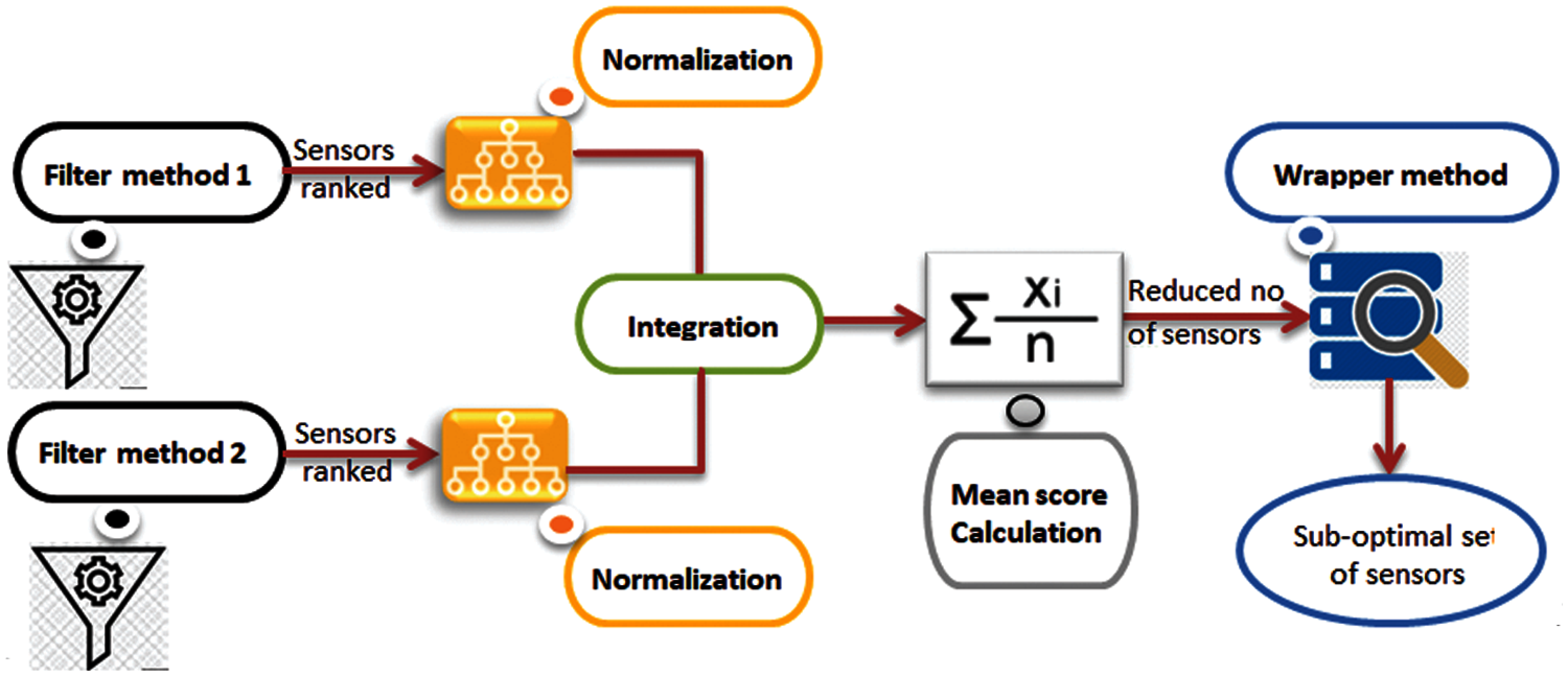
Figure 3: Hybrid sensor selection (HSS) technique
In the second step, scores are normalized to gain value in the range (0, 1). In the third step, scores are blended by computing the average of the two obtained scores. The calculated average threshold decision is used to isolate the significant sensors, hence, to minimize the dataset. In the fourth step, the dataset consists of only the already selected sensors are subjected to the following step of wrapper method.
The first filter method, is the Fisher score algorithm [17]. It selects sensors based on their scores using the chi-square method, which finally leads to the very well representative number of sensors that are ranked by their importance. Sensors with the highest Fisher scores as the subset of the optimal sensors are used for furthermore analysis. The second filter method is the ANOVA-test [18]. It is used to check the variance between sensors. In addition, compare the average value of more than two sensors by analyzing variances. After completing the two filter methods and set a score to each sensor according to its importance for the target. The dataset output should be normalized to obtain values in the range (0, 1). Hence, they are blended by taking the average value of the two scores calculated. Sensors with a score higher than the average score are selected.
The final step of the HSS technique is the wrapper method [19] (Exhaustive search method). It is used to select a sub-optimal set of sensors in a reasonable time without affecting the network functionality. The final datasets are extracted by finding the collection of sensors that provide the classifier's higher accuracy. Then, the LEF of the network is calculated.
The performance evaluation is achieved through the classification output based on both accuracy and lifetime extension factor (LEF). The classifiers K-NN, SVM, and RF, are used for the experimental study, as Fig. 4 indicates.
This stage's result exhibits the proposed HSS performance and its efficacy in LEF and classification accuracy phrases. The three intelligent classification algorithms’ overall performance is measured through the confusion matrix usage [20]. The matrix provides a vision of how well the classifier will perform on the processed dataset. For each experiment, the repeated k-fold cross-validation method is used to evaluate the proposed HSS performance using K = 10 with three repeats. Besides, overall performance metrics, like precision, recall, and F1-Score, can be obtained from this matrix.
In this work, seven different classifiers have been tested. Classifiers are namely Bagging, Random Forest (RF), Extra Trees (ET), Logistic Regression (LR), Decision Tree (DT), SVM, and K-NN. All classifiers showed good accuracy results. The highest accuracy records are accredited for SVM, K-NN, and RF classifiers. These three classifiers have been adopted in this paper to highlight the proposed HSS outperform.

Figure 4: Classifier techniques
Four experiments were performed on four distinct datasets. Each experiment is divided into three cases. In each case, the performance evaluation, such as the number of sensor selection, LEF, and accuracy, are measured to ensure the proposed HSS performance in different situations.
Energy-efficient management is mostly conceptualized as mechanisms and strategies by which the overall energy of the network is allocated, arranged, and used effectively by all sensors so that the network remains fully functional for its expected life. Since the WSNs energy is very restricted particularly in remote areas where obtaining additional energy is inconsequential because of the environmental feud. It is effective to achieve discreet equilibrium between energy supply and network load through energy conservation to avoid early energy exhaustion. As a result, designing a network with specific application requirements that satisfies the network lifetime remains a challenge. Individual sensor measurements report with highly correlated and irrelevant sensed data is energy consuming and memory inefficient due to the quality of the monitored conditions and the large number of sensors deployed. Therefore, schemes that manage network energy efficiently, at the data collection phase, are primary to the sustainability of the network. That is achieved by minimizing the amount of needless data collection through communication and hence, that will reduce energy dissipation and prolong the network lifespan.
All experiments were performed on AMD A10-8700P Radeon R6, 1.80 GHz, and an 8 GB of RAM running a 64-bit Windows 10 operating system. Software implementation has been performed on Anaconda 2019 using python 3.
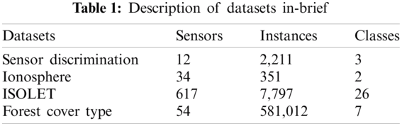
The four datasets used in this paper are downloaded from UCI and Kaggle machine learning repositories [21]. The Ionosphere dataset is a radar dataset gathered through Goose Bay, Labrador. It is grouped with a useful resource of 34 real sensor nodes and has two classes for radar signal. A forest cover type dataset was developed at the University of Colorado. It is used for predicting unknown regions. Sensor Discrimination is a labeled dataset and has three classes “group A,” “group B,” and “false alarm” Besides, ISOLET is a large dataset divided into five parts. A brief description of the datasets is provided in Tab. 1.
This experiment is performed on the Sensor Discrimination dataset that consists of 12 sensors and 2,212 instances. The recipient node must identify the unknown sample, then tag which category the unknown sample belongs to. Each sensor gets a score indicating its importance concerning the target. Fig. 5 illustrates the results using the fisher score based on the chi-square method after normalization. Moreover, it shows that many sensors have a high impact on the output, beginning with sensor F10 and ends with F12. The ANOVA test determines how much sensors are affecting the output. If the sensor's score is low, this sensor has no impact on the output and vice-versa. Fig. 6 shows each sensor's score using the ANOVA test method after normalization. Also, it indicates that the sensor F12 has the highest impact and F8 has the lowest impact on the output.

Figure 5: Fisher output after normalization for experiment one
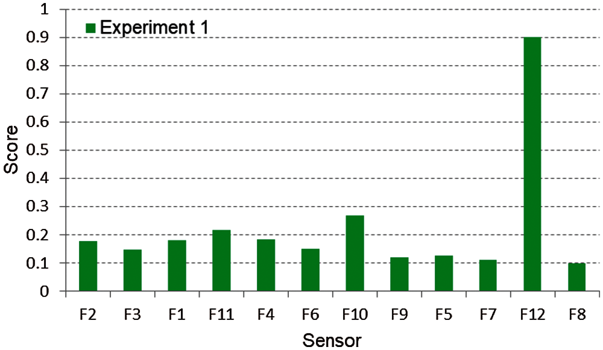
Figure 6: ANOVA test output after normalization for experiment one
After combining all sensor scores obtained from Fisher and ANOVA filters, the average of all combined sensors scores is calculated (equal to 1.032 in Experiment 1), as shown in Fig. 7. This average can be considered as the threshold decision. Hence, sensors’ scores are compared with the threshold value, and only sensors have scores greater than the threshold will pass to the next step. This process minimizes the dataset and extracts only the interesting sensors. This reduced dataset is used as an input data to the Wrapper exhaustive method to find the best combination of input sensors. The exhaustive search starts with looking for the best one-component subset of the input sensors. After that, it discovers the best two-component sensor subset, which might also consist of any pairs of the input sensors. Afterward, it continues to find the best triple out of all the collections of any three input sensors, etc. The best sensors selected are then used to evaluate the classifier accuracy level.

Figure 7: All sensors score after combining two methods for experiment one
Tab. 2 indicates the performance evaluation parameters, such as sensor selection, LEF, and accuracy before applying the proposed HSS technique. In experiment one regarding the sensor discrimination dataset; all 12 sensors were used before applying HSS. This can be considered the network LEF equal to 1, and the accuracy is 99%, 99%, and 98% for K-NN, RF, and SVM, respectively. However, after the HSS implementation, three cases were used to increase the network LEF with an acceptable accuracy level. For example, in case 1, with 2 out of 12 sensors are selected, the network LEF is increased to 6 times with an accuracy of 84%, 84%, and 83% for K-NN, RF, and SVM, respectively. While the best two sensors are F11 and F10 In cases 2 and 3, the network LEF increased to 4 and 2.4 times, respectively, with sensor selection of 4 and 5 out of 12.
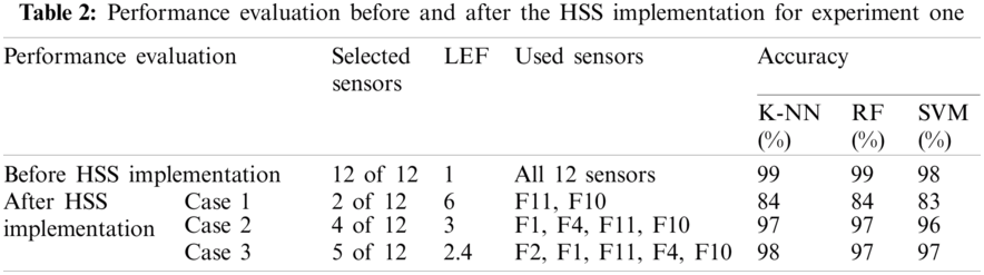
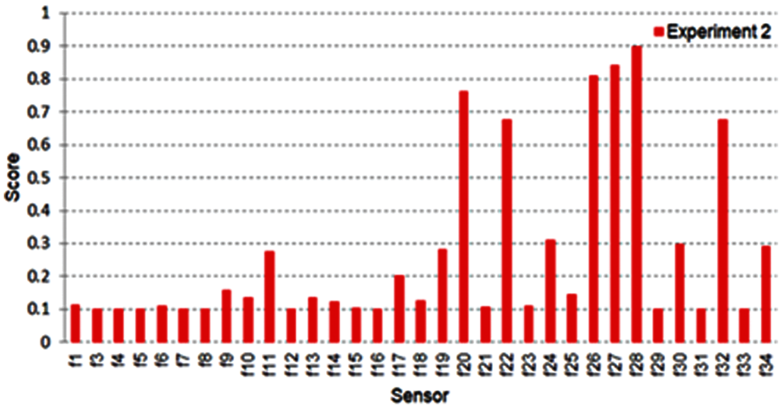
Figure 8: Fisher output after normalization for experiment two
This experiment is performed on the Ionosphere dataset. It is a radar dataset gathered from 34 several real sensor nodes and 351 instances/records. The same steps that were taken in experiment one are further implemented here. Fig. 8 shows fisher score output after normalization for experiment two. Fig. 9 shows the normalized ANOVA test output and the sensors’ score from f1 to f34. Many sensors take a score higher than 0.5, and this means several sensors will be chosen as the best. After combining these two filter methods, as in Fig. 10, the threshold decision is equal to 0.811. The sensors that have the highest output will be extracted. This process nominates a reduced dataset fed to the exhaustive search method to choose the best-selected number of sensors.
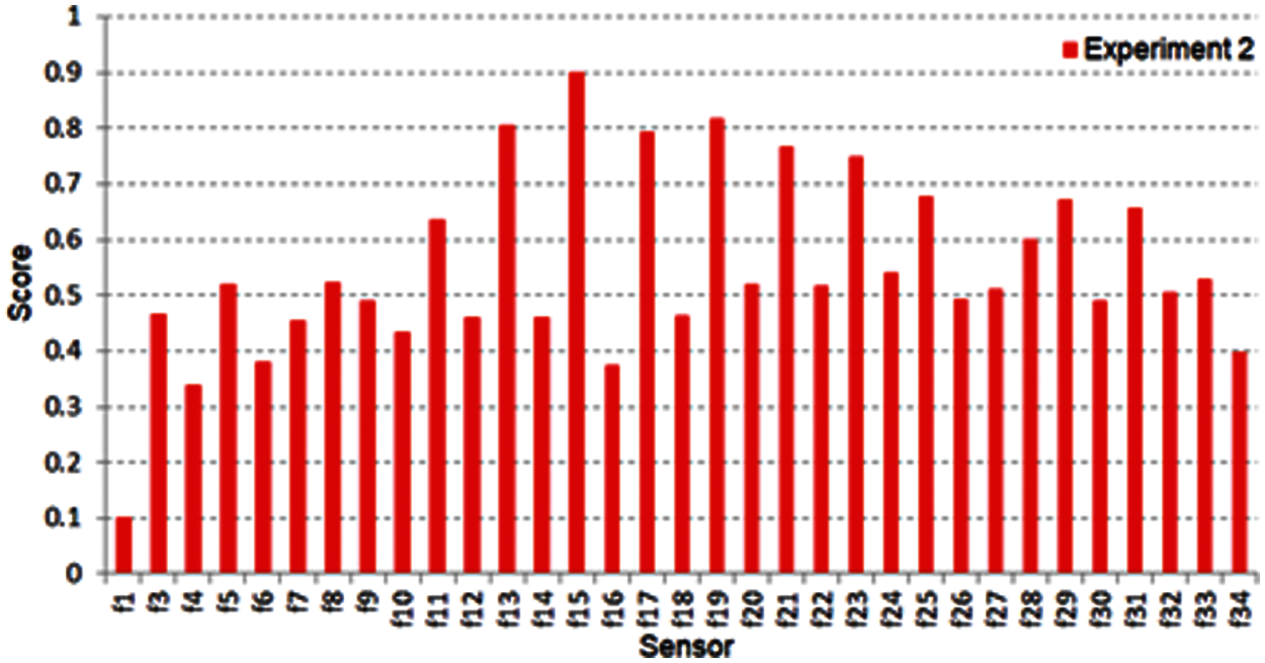
Figure 9: ANOVA test output after normalization for experiment two

Figure 10: All sensors score after combining two methods for experiment one
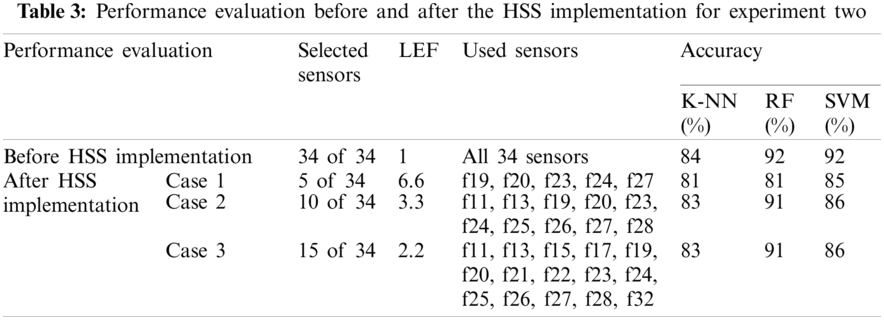
In experiment two, all 34 sensors were used before applying the proposed HSS technique. That is considered the network LEF equal to 1, and the accuracy is 84%, 92%, and 92% for K-NN, RF, and SVM, respectively. After the HSS implementation, three cases were used to increase the network LEF with an acceptable accuracy level. In case 1, 5 out of 34 sensors are selected, the network LEF is increased by 6.6 times with an accuracy of 81%, 81%, and 85% for K-NN, RF, and SVM, respectively. In cases 2 and 3, the network LEF increased by 3.3 and 2.2 times, respectively, with sensor selection of 10 and 15 and the accuracy level close to the results before applying the proposed HSS technique. All results obtained are shown in Tab. 3.
The motivation of ISOLET dataset is to predict which letter or name would be spoken. The ISOLET is a massive dataset with 7797 records and 617 sensors. It is divided into five parts. In this work, the Isolet5 dataset will only be used with 1559 records and 617 sensors due to the memory size limitation. For that specific reason, Fisher and ANOVA results were not presented because it has a lot of sensors to be shown, unlike the previous two datasets. For simplicity, the results will be mentioned after combining the two filter methods.
The proposed technique nominates 174 sensors that have a score higher than the average score of all sensors (threshold = 0.507). These 174 sensors are fed to the Exhaustive search method to select the best 10, 20, and 30 sensors as illustrated in Tab. 4.

Forest Cover is one of the biggest datasets processed in this work. The first 25000 recordings were chosen due to limited memory size. Unfortunately, these specific records were contained Nan values in some attributes like A15 and A25 sensors. Therefore, it was more convenient to select records in another way by sampling the whole dataset to overcome this issue. An (i + 1) sampling was convenient with a step of A15 didn't provide Nan values, and the number of selected records was about 39000 records. The same steps that were taken in experiments one, two, and three have been performed here. Fig. 11 shows the Fisher score output after normalization for experiment four. Eleven sensors achieved a high impact on the output, beginning with sensor A0 and ends with A53.

Figure 11: Fisher output after normalization for experiment four
Fig. 12 shows the highest two sensors’ scores, A5 and A9, according to the ANOVA test after normalization for experiment four. The average is similarly compared to nominate a reduced dataset consisting of 11 sensors, as shown in Fig. 13. This reduced data output was fed to the exhaustive search method and achieve A0, A5, and A9 as the best three sensors selected.

Figure 12: ANOVA test output after normalization for experiment four
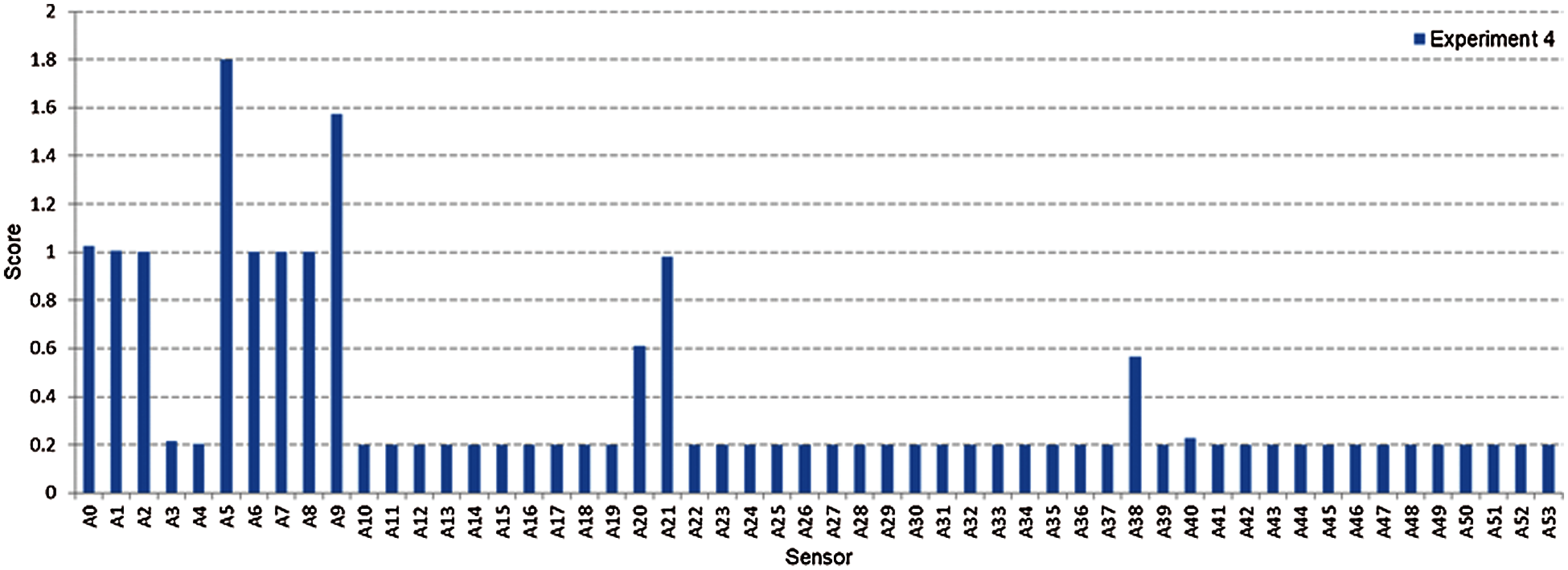
Figure 13: All sensors score after combining two methods for experiment four
In experiment four, all 54 sensors were used before applying the proposed HSS technique (LEF equal to 1), with accuracy of 86%, 90%, and 41% for K-NN, RF, and SVM, respectively. After the HSS implementation, three cases were considered to increase the network LEF with an acceptable accuracy level. In case 1, 3 out of 54 sensors are selected, the network LEF is increased by 18 times with an accuracy of 80%, 82%, and 40% for K-NN, RF, and SVM, respectively, where the best three sensors are A0, A5, and A9. In cases 2 and 3, the network LEF increased by 9 and 6.75 times, respectively, with 6 and 8 selected sensors. The accuracy level was close to the results before applying the proposed HSS technique. All obtained results are shown in Tab. 5.

The intelligent classification algorithms’ overall performance is measured through the use of the confusion matrix. This matrix shows a vision of how well the classifier would perform on the entered dataset. A variety of performance measures like accuracy, precision, recall, and F1-score, can be obtained from this matrix. Tab. 6 indicates the structure of the confusion matrix. Results of True Positive (TP), False Positive (FP), False Negative (FN), and True Negative (TN) are obtained. Accuracy is one measure to evaluate classification systems. It can be defined as the fraction of predictions that the model gets right. The definition of the accuracy as Eq. (2) shows:

In classification, the accuracy may be computed using positives and negatives measurements as Eq. (3):
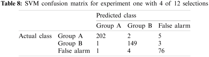
True Positives (TP) is the items where the actual class is positive and classified properly predicted to be positive. Similarly, True Negatives (TN) is the items where the actual class is negative and classified properly predicted to be negative. Contrarily, False Positives (FP) is the items where the actual class is negative and classified incorrectly predicted to be positive. Similarly, False Negatives (FN) is the items where the actual class is positive and classified incorrectly predicted to be negative. Tabs. 7 and 8 show the confusion matrices for Linear-SVM over the sensor discrimination dataset with a selection of 2, 4, and 5 out of 12 sensors. The sum of the diagonals represents the number of properly classified samples. For instance, the total number of properly classified samples for SVM is 366, that is, the sum of 185, 146, and 35. In this case, the accuracy is 366/443 × 100 = 83%, where the total number of instances in the testing dataset is 443. The accuracy calculated is 84% for K-NN with selection 2 out of 12 sensors. The same steps are applied for the remaining cases for more selected sensors with the proposed classifiers.

Tab. 9 illustrates Linear-SVM confusion matrices over the sensor discrimination dataset to select 5 out of 12 sensors. The total number of properly classified samples for SVM is 434 (sum of 201, 152, and 81). In this case, the accuracy is 427/443 × 100 = 98%, while the total number of records in the testing dataset is 443. Similarly, the accuracy calculated for K-NN is 99%.

The classification output shows precision, recall, and F1-score [22] given by SVM for the sensor discrimination dataset, selecting 2 out of 12 sensors shown in Tab. 10. Therefore, whenever building a model, the following parameters should help figure out how well the proposed model has performed. The precision is the rate of adequately predicted positive classes to all the predicted positive classes as Eq. (4). That reveals; of all classes labeled as group A, is how many are classified as group A. The high precision is related to the low rate of false positive. In this situation, it gives 0.91.

The recall is the rate of properly predicted positive classes to all observations in actual classes. That reveals; of all given classes in group A, It gets a recall of 0.94 that is suitable for this example as it's greater than 0.5, as Eq. (5) shows.
F1 score is the weighted-average of recall and precision. Hence, this value takes both FP and FN into consideration. It is unclear to be understood as accuracy; however, F1 is often more helpful than accuracy, particularly, if there is a dissimilar class classification. Accuracy acts better, whether FN and FP have identical costs. If either FN's or FP's value is very distinct, it's preferable to observe recall and precision. In group A case, the F1 score is 0.93, as Eq. (6) shows.
The number of selected sensors impacts the network LEF. If the selected sensor increases, the network LEF will be decreased. In the same time, the accuracy will be impacted during this process, and the network designers have to trade-off the accuracy for LEF using the best-tuned sensor selection. Fig. 14 shows the LEF and the number of sensor selections for all previous experiments. Researchers usually focus on the accuracy of the machine learning technique that they are using. Some of them, however, compare their findings to other available methods. As for the time performance, there are two parts. The first part is measuring the total time that is taken to build the training technique. The second part is measuring the total time that is taken to find the results based on the test data and both training and test data time are combined. Obviously, the accuracy results before HSS is better than after implementing HSS while, the reasons can be described as follows:
• The WSNs aren't operating with 100% of sensors.
• The WSNs designers or administrators have to trade-off the accuracy and the network lifetime by using the best-tuned sensor selection.
• Exploiting the acceptable tolerance in accuracy was the main idea of this research work. It is clearly demonstrated in the performance evaluation tables before and after the HSS implementation, the lifetime extension through energy conservation maintaining an acceptable accuracy measure.
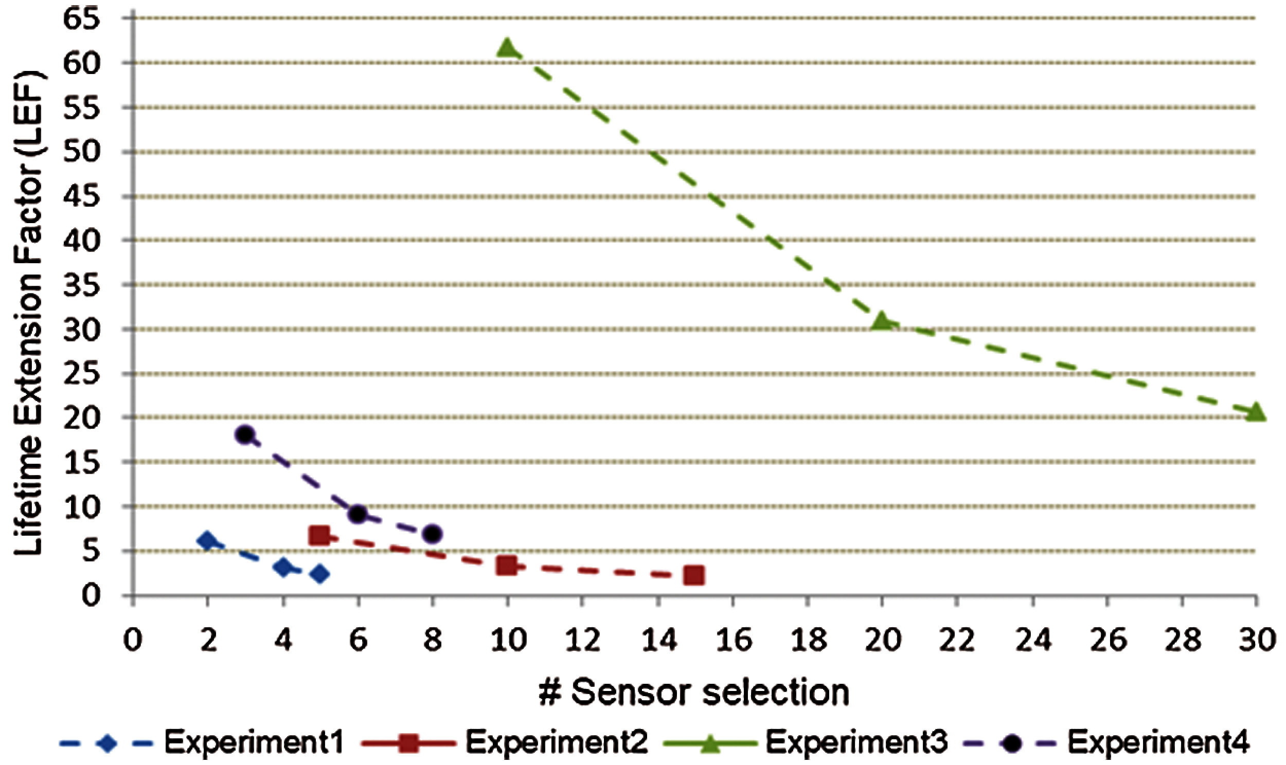
Figure 14: Lifetime extension factor of all experiments

Tab. 11 shows the average time, in seconds, taken before and after building the proposed HSS. The RF takes the largest time, 0.210 s, to build the technique before using the proposed HSS. After using the proposed HSS, RF takes less time in the three sensor selection cases. Also, the RF classifier takes more time compared to SVM and K-NN. For example, a longer time to experiment one accrued when five sensors were chosen. In this case, RF increased the time by a factor of 0.089 s compared with the K-NN classifier and 0.052 s compared with SVM. It is clear that the proposed HSS reduces the computational time required in each selection case.
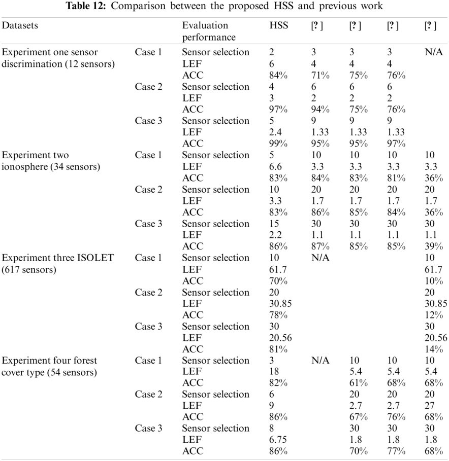
Tab. 12 shows the comparison between the proposed HSS and the previous work in WSNs energy conservation. This comparison used four datasets, namely Sensor discrimination, Ionosphere, ISOLET, and Forest cover type. In each dataset, there are three cases to demonstrate the superiority of the proposed HSS technique. In each case, three evaluation factors were used to compare between five studies regarding the number of sensor selections, the network LEF, and the accuracy level.
Experimental results indicated that, using the best classifier results in case 1 for the sensor discrimination dataset, the HSS technique reduced the number of selected sensors by 1 and doubled the network LEF. Moreover, it has achieved a higher accuracy level compared to other studies in the literature. Similar results are achieved for cases 2 and 3. In the Ionosphere dataset, the proposed HSS technique used half the number of sensors used in the previous work and can double the network LEF with an acceptable accuracy level. Furthermore, in the ISOLET dataset, HSS used the same selected sensors in [12] and presented the same LEF with a higher accuracy. The superiority of HSS demonstrated that in Forest cover type dataset, using a number of sensors less than 50% of used sensors in [7,12,14] and double LEF with higher accuracy level.
This paper proposes an intelligent HSS technique for efficient-energy conservation in WSNs. Besides, it selects a subset of sensors to increase the network lifetime by removing redundant, noisy, or irrelevant sensors. The proposed HSS technique combines two filter methods and a wrapper method for sensor selection. The HSS technique provides a larger informative subset at an acceptable time. Furthermore, it could be used in all kinds of datasets with no prior assumption of the data and appropriate to big or imbalanced datasets. The HSS has been used effectively on several datasets from the UCI and Kaggle repositories such as Sensor Discrimination, Ionosphere, ISOLET, Forest Cover Type, and. In each dataset, three cases were considered to demonstrate the superiority of the HSS technique. Moreover, in each case, three evaluation factors were highlighted to compare five different previous works in terms of the number of sensors selected, the network LEF, and the accuracy level. Evaluation results indicated that the proposed HSS technique could double the network lifetime and increase the accuracy by more than 20% with the minimum number of sensors corresponding to the previous methodologies without affecting the network functionality. For future work, the classifier's performance using different benchmark datasets with several kernels, like sigmoid or Gaussian, will be investigated. Moreover, this work will be committed to various purposes such as prediction and clustering purposes. It would also be desirable to extend the experiments to include more datasets acquired from real WSNs high-dimensional data.
Funding Statement: The authors received no funding for this study.
Conflicts of Interest: The authors declare that they have no conflicts of interest to report regarding the present study.
1. M. A. Alsheikh, S. Lin, D. Niyato and H. P. Tan, “Machine learning in wireless sensor networks: Algorithms, strategies, and applications,” IEEE Communications Surveys and Tutorials, vol. 16, no. 4, pp. 1996–2018, 2014.
2. W. Zhang, W. Fang, Q. Zhao, X. Ji and G. Jia, “Energy efficiency in internet of things: An overview,” Computers, Materials & Continua, vol. 63, no. 2, pp. 787–811, 2020.
3. D. K. Bangotra, Y. Singh and A. Selwal, “Machine learning in wireless sensor networks: Challenges and opportunities,” in Proc. PDGC, Solan, India, pp. 534–539, 2018.
4. M. M. Ahmed, A. Taha, A. E. Hassanien and E. Hassanien, “An optimized k-nearest neighbor algorithm for extending wireless sensor network lifetime,” Advances in Intelligent Systems and Computing, vol. 723, pp. 506–515, 2018.
5. S. Zidi, T. Moulahi and B. Alaya, “Fault detection in wireless sensor networks through SVM classifier,” IEEE Sensors Journal, vol. 18, no. 1, pp. 340–347, 2018.
6. Z. Noshad, N. Javaid, T. Saba, Z. Wadud, M. Saleem et al., “Fault detection in wireless sensor networks through the random forest classifier,” Sensors (Switzerland), vol. 19, no. 7, pp. 1–21, 2019.
7. K. M. Fouad and D. L. El-Bably, “Intelligent approach for large-scale data mining,” International Journal of Computer Applications in Technology, vol. 63, no. 2, pp. 93–113, 2020.
8. A. Y. Barnawi and I. M. Keshta, “Energy management in wireless sensor networks based on naive Bayes, MLP, and SVM classifications: A comparative study,” Journal of Sensors, vol. 2016, 2016.
9. X. He, D. Cai and P. Niyogi, “Laplacian score for feature selection,” Advances in Neural Information Processing Systems, vol. 18, pp. 507–514, 2005.
10. W. I. Gabr, M. A. Ahmed and O. M. Salim, “Hybrid detection algorithm for online faulty sensors identification in wireless sensor networks,” IET Wireless Sensor Systems, vol. 10, no. 6, pp. 265–275, 2020.
11. A. T. Azar, A. M. Anter and K. Fouad, “Intelligent system for feature selection based on rough set and chaotic binary grey wolf optimisation,” International Journal of Computer Applications in Technology, vol. 63, no. 2, pp. 4–24, 2020.
12. B. O. Ayinde and A. Y. Barnawi, “Energy conservation in wireless sensor networks using partly-informed sparse autoencoder,” IEEE Access, vol. 7, pp. 63346–63360, 2019.
13. M. Alwadi and G. Chetty, “Feature selection and energy management for wireless sensor networks,” International Journal of Computer Science and Network Security, vol. 12, no. 6, pp. 46–51, 2012.
14. Y. Li, Y. Wang and G. He, “Clustering-based distributed support vector machine in wireless sensor networks,” Journal of Information and Computational Science, vol. 9, no. 4, pp. 1083–1096, 2012.
15. A. Y. Barnawi and I. M. Keshta, “Energy management of wireless sensor networks based on multi-layer perceptrons,” in Proc. EWE, Berlin, Offenbach, Germany, pp. 939–944, 2014.
16. J. Kang, J. Kim, M. Kim, and M. Sohn, “Machine learning-based energy-saving framework for environmental states-adaptive wireless sensor network,” IEEE Access, vol. 8, pp. 69359–69367, 2020.
17. S. M. Saqlain, M. Sher, F. A. Shah, I. Khan, M. U. Ashraf et al., “Fisher score and matthews correlation coefficient-based feature subset selection for heart disease diagnosis using support vector machines,” Knowledge and Information Systems, vol. 58, no. 1, pp. 139–167, 2019.
18. S. F. Sawyer, “Analysis of variance: The fundamental concepts,” The Journal of Manual & ManipulaTive Therapy, vol. 17, no. 2, pp. 27–38, 2013.
19. R. Kohavi and G. H. John, “Wrappers for feature subset selection,” Artificial Intelligence, vol. 97, no. 2, pp. 273–324, 1997.
20. A. K. Santra and C. J. Christy, “Genetic algorithm and confusion matrix for document clustering,” International Journal of Computer Science Issues, vol. 9, no. 1, pp. 322–328, 2012.
21. A. Frank and A. Asuncion, “UCI machine learning repository,” Irvine, CA, University of California, School of Information and Computer Science, Accessed on Feb. 09, 2021. [Online]. Available: https://archive.ics.uci.edu/ml/index.php.
22. M. Sokolova and G. Lapalme, “A systematic analysis of performance measures for classification tasks,” Information Processing and Management, vol. 45, no. 4, pp. 427–437, 2009.
 | This work is licensed under a Creative Commons Attribution 4.0 International License, which permits unrestricted use, distribution, and reproduction in any medium, provided the original work is properly cited. |