Computers, Materials & Continua DOI:10.32604/cmc.2022.020954
Article

Position Control of Flexible Joint Carts Using Adaptive Generalized Dynamics Inversion

Ibrahim M. Mehedi1,2,*, Mohd Heidir Mohd Shah1, Soon Xin Ng3, Abdulah Jeza Aljohani1,2, Mohammed El-Hajjar3 and Muhammad Moinuddin1,2

1Department of Electrical and Computer Engineering (ECE), King Abdulaziz University, Jeddah, 21589, Saudi Arabia
2Center of Excellence in Intelligent Engineering Systems (CEIES), King Abdulaziz University, Jeddah, 21589, Saudi Arabia
3Next Generation Wireless Research Group, University of Southampton, UK
*Corresponding Author: Ibrahim M. Mehedi. Email: imehedi@kau.edu.sa
Received: 16 June 2021; Accepted: 17 July 2021

Abstract: This paper presents the design and implementation of Adaptive Generalized Dynamic Inversion (AGDI) to track the position of a Linear Flexible Joint Cart (LFJC) system along with vibration suppression of the flexible joint. The proposed AGDI control law will be comprised of two control elements. The baseline (continuous) control law is based on principle of conventional GDI approach and is established by prescribing the constraint dynamics of controlled state variables that reflect the control objectives. The control law is realized by inverting the prescribed dynamics using dynamically scaled Moore-Penrose generalized inversion. To boost the robust attributes against system nonlinearities, parametric uncertainties and external perturbations, a discontinuous control law will be augmented which is based on the concept of sliding mode principle. In discontinuous control law, the sliding mode gain is made adaptive in order to achieve improved tracking performance and chattering reduction. The closed-loop stability of resultant control law is established by introducing a positive define Lyapunov candidate function such that semi-global asymptotic attitude tracking of LFJC system is guaranteed. Rigorous computer simulations followed by experimental investigation will be performed on Quanser's LFJC system to authenticate the feasibility of proposed control approach for its application to real world problems.

Keywords: Adaptive control; generalized dynamic inversion; moore-penrose generalized inverse; sliding mode control; lyapunov stability; semi-global asymptotic stability

1  Introduction

This paper presents a controller design for position tracking of a classroom equipment for mass-damper-spring quadratic systems called Linear Flexible Joint Cart (LFJC) system supplied by [1]. Due to some non-parametric uncertainties, the controller must be designed with adaptive mechanism. Adaptive controller designs remain an active field of research as systems nowadays were designed to be more complex. Parameter estimation techniques are the fundamental of adaptive control system and the way the estimated parameter is used determines their classification. Adaptive control system can be classified either as direct method when the estimated parameters are used directly in the controller, or indirect method when they were used only to calculate required controller parameters or hybrid method which is a mix between the first two.

One of the most popular adaptive controllers is the Model Reference Adaptive Controller (MRAC) which belongs to the direct adaptive control method. MRAC has a structure where an additional control loop called adaptation loop is added to the normal feedback structure to adapt to changes in the system dynamic as well as to compensate disturbances. Since its first implementation in 1958, MRAC has evolved and some of recent works on the controller can be found in [2–4].

One type of adaptive controller under the family of indirect method is Model identification Adaptive Control (MIAC). The working principle of MIAC is to optimize the performance of a controller by identifying the system while it is running. This is very much similar to the concept of Self-tuning Regulators (STR) [5], in fact, the term MIAC was proposed to solve the interpretation issue of STR with another controller having similar concept called Self-optimizing Adaptive Control (SOAC) [6]. An example of MIAC implementation on Unmanned Aerial Vehicle (UAV) is discussed in [7].

The two controllers discussed earlier used single model as reference, there exist a type of adaptive controller that uses large number of models as references called Multi-model Adaptive Control (MMAC). Not all reference models will be used all the time though. At an instance, only one model that is closest to the plant is chosen. Recent examples of MMAC implementation include a Dynamic Positioning System for Quadrotor Helicopters and Simulator for Solid Oxide Fuel Cell Gas Turbine Power Plants [8,9]. There are also some proposals for a two-layer switching strategy in MMAC [10] and artificial intelligent (AI) based switching techniques such as fuzzy logic [11] and neural networks [12].

The usage of AI based technique in adaptive control is tempting as it generally provides a model free universal approximation. They were typically used together with classical controller to enhance their robustness, adaptivity to changes, and improve non-linear model approximation. Some examples are the adaptive fuzzy PID [13], adaptive fuzzy sliding mode [14], and neural adaptive PID [15].

There is still an exhaustive list of types of adaptive controller yet to discussed in this paper like gain scheduling, iterative learning control, adaptive pole placement, and extremum-seeking controllers. A brief review on the state-of-the art adaptive control systems can be found in [16–18].

In this paper, an inversion based AGDI control approach is applied for linear position control of LFJC system. A Moore-Penrose Generalized Inverse was used to parameterize the solution as the inversion could results in infinite number of solutions as given in [19–21]. An additional term based on Sliding Mode Controller (SMC) is included in the proposed controller as implemented in [19]. In all these references, a constant sliding mode gain is used in the additional term for its application to rotary servo cart and inverted pendulum systems. However, in this article, the authors have extended the previous work by implementing the adaptive sliding mode gain in the discontinuous control which adapts itself with respect to the changing environment for chattering reduction and to achieve improved tracking performance. The article has presented very first time the application of AGDI control on Quanser's LFJC system and the performance has been verified through both numerical simulations and experimental investigations. In Section 4, in-depth stability analysis of the controller has been presented to guarantee semi global asymptotic tracking performance. Results from computer simulations and practical experiments will be discussed in detail in Section 5. Finally, the paper is concluded in Section 6.

2  Mathematical Model of Linear Flexible Joint Cart System

An LFJC system as shown in Fig. 1 is a system of two carts sliding on a track with one of the carts is driven by a DC motor. It can be modelled as a two mass-spring system as illustrated in the schematic diagram in Fig. 2 where mc and mjc is the mass of the cart and the joint cart respectively, while xc and xjc is their respected position. The position of the cart is measured using a quadrature optical encoder. The linear force applied to the cart is denoted by Fc whereas the spring linking the two carts has a constant denoted by Ks

Figure 1: Linear flexible joint cart system [1]

Figure 2: Schematic of LFJC

The differential equations of the system are given as:

x¨c=1Jeq(−Ksxc+Ksxjc−Beqx˙c+Fc)(1)

and

x¨jc=1mjc(Ksxc−Ksxjc−Beqjcx˙jc)(2)

where Beq and Beqjc are the equivalent viscous damping of the servo system and the LFJC respectively while Jeq is the equivalent moment of inertia. The linear force, Fc which is generated by the servo motor can be described by the following equation:

Fc=ηgKgKtRmrmp(−KgKmx˙crmp+ηmVm)(3)

The servo motor parameters in [3] are as defined in [1]. We can re-write (1) and (2) in the state-space form as in the following:

x˙=Ax+Bu(4)

and

y=Cx+Du(5)

where

A=[00100001−KsJeqKsJeq−BeqJeq0Ksmjc−Ksmjc0−Beqjcmjc](6)

B=[001Jeq0](7)

C=[10000100](8)

D=[00](9)

while the state variables and control variable are as follows:

xT=[xc||xjc||x˙c||x˙jc](10)

and

u=Vm(11)

3  Controller Design

To track the linear position of LFJC system, a controller is designed to have two loops as shown in Fig. 3. In the outer loop, we employed an AGDI control law to provide position signal commands while the inner loop will use the signals to generate the required voltage to move the linear cart to its desired position.

3.1 GDI Control Law

[x¨cd+KsJeqxc−KsJeqxjc+BeqJeqx˙c−c1ex˙c−c2ex¨cx¨jcd−Ksmjcxc+Ksmjcxjc+Beqjcmjcx˙jc−c3ex˙jc−c4ex˙jc]=[1Jeq0]Vm(12)

By formulating constant time ordinary differential constraints, we begin our controller design:

e¨xc=c1(t)e˙xc+c2(t)exc(13)

e¨xjc=c1(t)e˙xjc+c2(t)exjc(14)

where, ci(i=1 to 4) are coefficients whose value should be selected appropriately in order for the constraint differential equation to achieve asymptotic stability. The term exc=n1(xca−xcd)2 in (13) is an error function for the cart's position where and d denotes the actual and desired values. Similarly, the error function for the joint cart's position in (14) is exjc=n2(xjca−xjcd)2. n1 and n2 on the other hand are positive real valued constant.

Figure 3: Proposed controller architecture

To obtain the desired control action Vm, we utilize a dynamic inversion technique in which the dynamic equation should be in the form of:

M=NVm(15)

From the system's dynamic model in (6) and (7) and the constraint equations developed in (13) and (14), we can realize (15) by writing:

Now, we can obviously solve Vm by bringing the term N in (12) to the left and therefore invert it. This can't be done using the ordinary way as N is not a square matrix. To solve this issue, we apply a generalized method called the Moore-Penrose Generalized Inverse [18] as follows:

N+=NTNTN(16)

However, there can exists infinite number of solutions for Vm, therefore by using the Greville method, the solution is parameterized as in the following:

Vm=N+M+Pλ(17)

where λ is the null control and P is the null projection given by the following equation:

P=I−N+N(18)

Note that, the same control law is applied in both controller loops.

3.2 Robust Controller Design

In order to make the controller more robust, a technique similar to SMC is employed to augment the controller. For that, a set of sliding surface vector function for both outer and inner controller loop is defined as in the following:

So=[SxcoSxjco]=[e˙xco+c1(t)exco+c2(t)∫⁡excodotexjco+c3(t)exjco+c4(t)∫⁡exjco](19)

Si=[SxciSxjci]=[e˙xci+c1(t)exci+c2(t)∫⁡excidotexjci+c3(t)exjci+c4(t)∫⁡exjci](20)

Therefore, the derivative of the vector functions are as follows:

S˙o=[S˙xcoS˙xjco]=[e¨xco+c1(t)e˙xco+c2(t)excoe¨xjco+c1(t)e˙xjco+c2(t)exjco](21)

S˙i=[S˙xciS˙xjci]=[e¨xci+c1(t)e˙xci+c2(t)excie¨xjci+c1(t)e˙xjci+c2(t)exjci](22)

Note that subscripts i and o is used to represent the inner and outer loop part of the controller respectively. By setting the derivatives of the sliding functions as in (21) and (22) to 0, the constraint dynamic equations in (13) and (14) can now realize its asymptotic stability. This leads to the following definition:

S˙=NVm−M(23)

Finally, based on the sliding vector functions in (19) and (20) and considering the expression in (17), our switching control law was derived based on the rate achieving law, yielding the following:

Vmo∗=N+M+Poλo−CoN+So||So||(24)

Vmi∗=N+M+Piλi−CiN+Si||Si||(25)

where Co and Ci are the gains for both outer and inner loop of the controller. The adaptive mechanism of these gains will be discussed in the next sub-chapter.

3.3 Adaptive Controller Design

The designed controller were made adaptive by introducing an update mechanism for the gains in (24) and (25) which equations given as follows:

Co=||Vmoeq||TC^o+ηo(26)

Ci=||Vmieq||TC^i+ηi(27)

where Vmoeq and Vmieq represent the nominal GDI controllers given by (24) and (25) respectively while ηo and ηi ensure the reaching condition by bounding the disturbances. C^o and C^i are the adaptive modulation gains which the update mechanism is given as:

C^˙o=k1C^o+k2ϵo||Vmoeq||||So||(28)

C^˙i=k3C^i+k4ϵi||Vmieq||||Si||(29)

with k1, k2, k3, k4, and ϵo, ϵi are all constant positive scalar gains.

4  Stability Analysis

To guarantee stability of the controller, the error vectors exco, exjco, exci, exjci must be converge finitely. For that, the value of Co and Ci must be carefully selected. By substituting equation in (24) and (25) into (23), the following will be obtained:

S˙o=N(N+M+Poλo−CoN+So||So||)−M(30)

S˙i=N(N+M+Piλi−CiN+Si||Si||)−M(31)

Substitute P=I−N+N into (30) and (31) yields:

S˙o=(πN−I)M−πNCoSo||So||(32)

S˙i=(πN−I)M−πNCiSi||Si||(33)

where πN=NN+≠1 and I is an identity matrix. Based on the expression in (16), we can conclude that:

0<||πN||<1(34)

for all N≠0, and

limt→∞⁡πN=0↔limt→∞⁡N=0(35)

Next, we intend to prove that the sliding mode dynamics S˙ in (32) and (33) can achieve asymptotically stability by performing Lyapunov stability analysis.

Let the positive definite Lyapunov energy function is defined as:

V=12STS(36)

By substituting the (32) and (33) into the derivatives of Lyapunov function in (36) yields the following:

V˙o=SoT((πN−I)M−πNCoSo||So||)(37)

V˙i=SiT((πN−I)M−πNCiSi||Si||)(38)

According to the Lyapunov's direct method, asymptotic stability stability of S can be guaranteed when V˙ is negative definite therefore, Co and Ci must satisfies the following:

Co=||Vmoeq||TC^o+ηo>πN−1πN|M|(39)

Ci=||Vmieq||TC^i+ηi>πN−1πN|M|(40)

The sliding mode dynamics in (30) and (31) can be converged as the error vector e converge which as a result implying the condition in (35). Therefore:

lime→0⁡πN−1πN=−∞(41)

It can be observed that from (41) that it is not possible to obtain SMC gains which guarantees asymptotic stability. However, with suitable selection of the gains, we can let the controller to achieve a semi global practical stability. Let us assess the outer loop controller case according to the following theorem:

Theorem 1: for every real number πN∗∈(0,1) there exists a real number ηo∗>0 such that the time derivative of V along the solution trajectories of the sliding mode dynamic given by (32) is strictly negative for all πN>πN∗ and ηo>ηo∗

Proof: Define πN∗∈(0,1) , while η¯0 is defined as in the following:

η¯0=πN∗−1πN∗|M|(42)

It follows that η¯o>ηo. whenever πN>πN∗. Accordingly let Do be a neighbourhood of (exc,exjx=(0,0), and choose sliding gain constant ηo∗ such that

ηo∗>maxDoηo¯(43)

Then V˙o<0 holds true along any closed loop trajectory that initiates within Do whener πN>πn∗ existence of a finite number ηo∗ is guaranteed for any domain Do because M is globally bound which eventually leads to globally bounded exc and exjc trajectories respectively.

Theorem 2: Consider the closed-loop dynamical system of the LFJC given by (6) and (7). If the controlled voltage Vm given by (24) is applied, then the equilibrium point e=0 of the closde-loop dynamics is semi-globally practically stable.

Proof: To prove Theorem 1, the matrix bound ||πN∗|| can be arbitrarily selected closer to zero by choosing the gain such that V˙o<0, whenever the specified condition πN≥πN∗ is satisfied, the bound holds along any closed-loop trajectory in the neighbourhood D of e=0. In order for an error state trajectory e to fall within the defined domain πN<πN∗ in finite time and prevail within that domain, it follows that reducing the value of ||πN∗|| arbitrarily closer to zero implies driving the error vector e arbitrarily closer to zero and making it uniformly ultimately bounded, i.e., making practically e stable. Moreover, because Do can be arbitrarily expanded by increasing Co, then this practical stability is semi-global.

5  Results

To evaluate the performance of the designed controller, we perform numerical simulations with step and sine wave input. The same scenario is then repeated in the practical experiment on a real system. Two other controllers namely the GDI and Linear Quadratic Regulator (LQR) were also developed and tested in both simulations and experiments to provide comparison to the designed controller.

5.1 Simulation Results

The LFJC system is simulated based on the dynamic model given in (6–9) with the parameter's value given in [1]. First, the system model is tested with 0.2 Hz square-wave input with amplitude at 0.02 m. Results as shown in Fig. 4a demonstrates that the cart able to track the reference input when the proposed controller is employed. This was achieved with minimum oscillation as suggested by the results in Fig. 4b.

Figure 4: Simulation response of (a) xc and (b) xjc on square-wave input

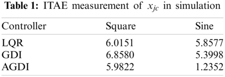
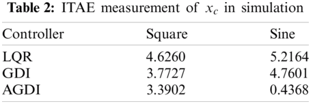
Then, sine-wave is used with the same frequency and amplitude as in the previous simulation and the results is as shown in Fig. 5. Here, the superiority of the proposed controller over GDI and LQR are obvious. The proposed controller's adaptivity is also evident especially for joint cart position as shown in Fig. 5b where a little oscillation was only observed in the first 1.5 s it before smoothly follows the set-point. The superiority of AGDI over the other two controllers are further proven by comparing their Integral Time Absolute Error (ITAE) as shown in Tabs. 1 and 2.

Figure 5: Simulation response of (a) xc and (b) xjc on sine-wave input

The input voltage generated in response to the set-point is shown in Fig. 6. Despite a little spike recorded in response to the square-wave set-point when the cart started to change its position, the voltage input was well within the allowable limits.

5.2 Experimental Results

The same scenario as in the simulation is tested on a real equipment where the experimental set-up is as shown in Fig. 7. The set-up consists of a Linear Flexible Joint Cart system as described in Section 2, an amplifier to provide sufficient power to the motor and sensors, and DAQ board for transmitting control signals from Matlab interface to the system and receiving measured data from the encoders.

Figure 6: Input voltage generated in response to (a) square-wave, (b) sine-wave set-point in simulation

Figure 7: LFJC experimental set-up

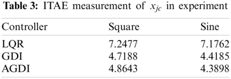
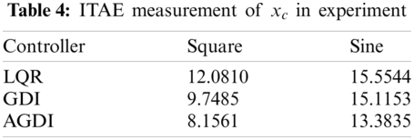
The experimental results for the proposed controller are shown in Fig. 8 for square-wave reference input and in Fig. 9 for sine-wave reference input. It can be observed from the results that the performance of all controllers was not as good as in the simulation especially with sine-wave reference input. The proposed controller, however, performs the best compared to the other two with LQR at the other end. This fact is backed by the ITAE measurement as shown in Tabs. 3 and 4.

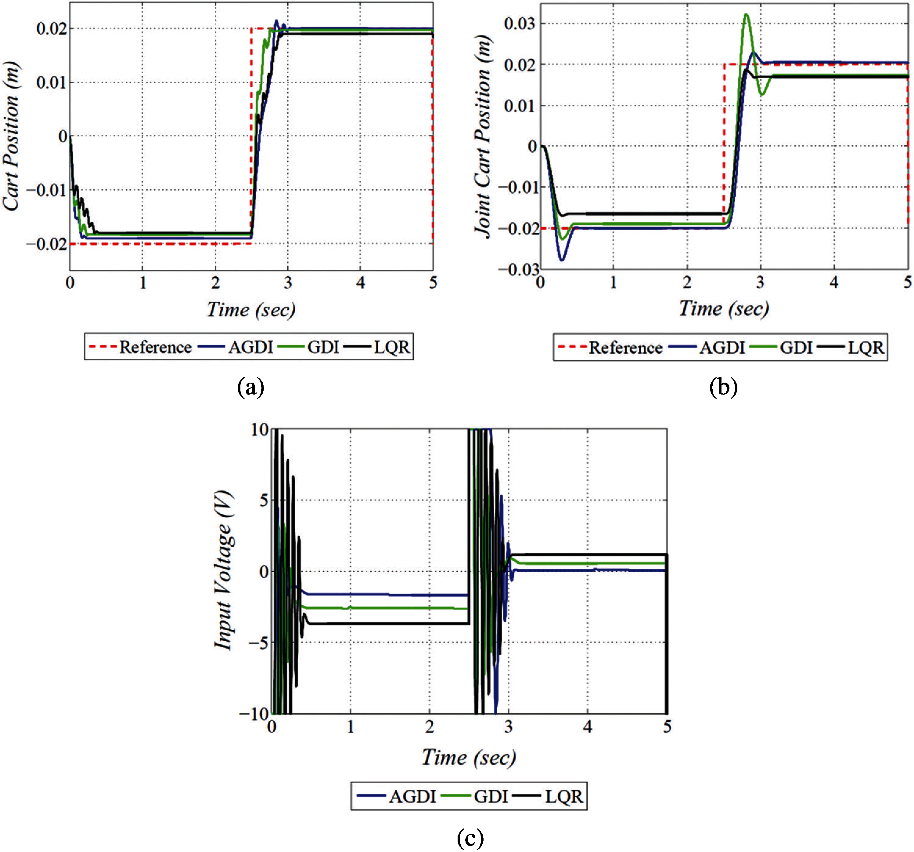
Figure 8: Square wave cases (a) cart position vs. time (b) joint cart position vs. time (c) input voltage vs. time

Figure 9: Sine-wave cases (a) cart position vs. time (b) joint cart position vs. time (c) input voltage vs. time

Figs. 8c and 9c show the input voltage generated in response to the input reference during the experiment. For square-wave set-point, it is similar to the one in simulation where voltage spike followed by a little oscillation is recorded when the cart starts to move except that this time the voltage spike produced by LQR was too high that it could harm the system. On the other hand, the input voltage oscillates almost all the time in order for the cart to move continuously to track the sine-wave input reference.

6  Conclusion

A two-loops adaptive controller based on GDI has been successfully implemented in tracking the linear position of LFJC system. The proposed AGDI control law contains two control elements. Laws of Control established using a baseline (continuous) control law designed to reflect control objectives. The baseline law derives from the conventional GDI approach and is based on the rules for GDI. By applying Moore-Penrose generalized inversion to the prescribed dynamics, the control law is established. The introduction of adaptation modulation gain has made the controller able to adapt to changes in the system. The superiority of the proposed controller over GDI and LQR was proven by the simulation and practical experimental results. However, there are still room for improvements especially in minimizing the oscillation produced by the input voltage due to the continuous movement of the cart.

Acknowledgement: This research work was funded by Institutional Fund Project under Grant No. (IFPHI-106-135-2020). Therefore, authors gratefully acknowledge technical and financial support from the Ministry of Education and King Abdulaziz University, DSR, Jeddah, Saudi Arabia.

Funding Statement: This research work was funded by Institutional Fund Projects under Grant No. (IFPHI-106-135-2020).

Conflicts of Interest: The authors declare that they have no conflicts of interest to report regarding the present study.

References

 1.  Quanser. IP02 User Manual, Quanser Inc., 2009.

 2.  E. H. Skorina, M. Luo, W. Tao, F. Chen, J. Fu et al., “Adapting to flexibility: Model reference adaptive control of soft bending actuators,” IEEE Robotics and Automation Letters, vol. 2, no. 2, pp. 964–970, 2017.

 3.  E. Arabi, B. C. Gruenwald, T. Yucelen and N. T. Nguyen, “A set-theoretic model reference adaptive control architecture for disturbance rejection and uncertainty suppression with strict performance guarantees,” International Journal of Control, vol. 91, no. 5, pp. 1195–1208, 2018.

 4.  Y. Mfoumboulou and R. Tzoneva, “Development of a model reference digital adaptive control algorithm for a linearized model of a nonlinear process,” International Journal of Applied Engineering Research, vol. 13, no. 23, pp. 16662–16675, 2018.

 5.  K. J. A°stro¨m and B. Wittenmark, “On self tuning regulators,” Automatica, vol. 9, no. 2, pp. 185–199, 1973.

 6.  R. Isermann, “Techniques in dynamics systems parameteradaptive control,” Control and Dynamic Systems V26: Advances in Theory and Applications, vol. 26, pp. 119, 2012.

 7.  Z. O¨reg, H. S. Shin and A. Tsourdos, “Model identification adaptive control-implementation case studies for a high manoeuvrability aircraft,” in 27th Mediterranean Conf. on Control and Automation (MEDAkko, Israel, pp. 559–564, 2019.

 8.  Z. S. Mahmoud and S. M. Raafat, “Robust multiple model adaptive control for dynamic positioning of quadrotor helicopter system,” Engineering and Technology Journal, vol. 36, no. 12 Part (A) (Engineering), pp. 1249–1259, 2018.

 9.  A. Tsai, P. Pezzini, D. Tucker and B. M. Kenneth, “Multiple-model adaptive control of a hybrid solid oxide fuel cell gas turbine power plant simulator,” J. Electrochem. En. Conv. Stor, vol. 16, no. 3, pp. 031003, 2019.

10. J. Xie, D. Yang and J. Zhao, “Multiple model adaptive control for switched linear systems: A two-layer switching strategy,” International Journal of Robust and Nonlinear Control, vol. 28, no. 6, pp. 2276–2297, 2018.

11. B. Kharabian, H. Bolandi, S. M. Smailzadeh and S. K. Mousavi Mashhadi, “Fuzzy switching for multiple model adaptive control in manipulator robot,” Journal of Automation Mobile Robotics and Intelligent Systems, vol. 11, no. 1, pp. 53–56, 2017.

12. J. Li, W. Zhang and Q. Zhu, “Weighted multiple-model neural network adaptive control for robotic manipulators with jumping parameters,” Complexity, vol. 2020, pp. 1–12, Article ID 3172431, 2020.

13. M. H. Shah, M. F. Rahmat, K. Danapalasingam and N. Wahab, “PLC based adaptive fuzzy PID speed control of dc belt conveyor system,” International Journal on Smart Sensing & Intelligent Systems, vol. 6, no. 3, pp. 1133–1152, 2013.

14. T. Yoshimura, “Design of an adaptive fuzzy sliding mode control for uncertain discrete-time nonlinear systems based on noisy measurements,” International Journal of Systems Science, vol. 47, no. 3, pp. 617–630, 2016.

15. H. R. Nohooji, “Constrained neural adaptive PID control for robot manipulators,” Journal of the Franklin Institute, vol. 357, no. 7, pp. 3907–3923, 2020.

16. S. G. Anavatti, F. Santoso and M. A. Garratt, “Progress in adaptive control systems: Past, present and future,” in 2015 Int. Conf. on Advanced Mechatronics, Intelligent Manufacture and Industrial Automation, IEEE, Surabaya, Indonesia, pp. 1–8, 2016.

17. G. Ahmed, S. Islam, I. Ali, I. A. Hayder, A. Ibrahim et al., “Adaptive power control aware depth routing in underwater sensor networks,” Computers, Materials & Continua, vol. 69, no. 1, pp. 1301–1322, 2021.

18. X. He, H. Jiang, Y. Song and M. Owais, “Power control and routing selection for throughput maximization in energy harvesting cognitive radio networks,” Computers, Materials & Continua, vol. 63, no. 3, pp. 1273–1296, 2020.

19. I. M. Mehedi, U. Ansari and U. M. Al-Saggaf, “Three degree of freedom rotary double inverted pendulum stabilization by using robust generalized dynamic inversion control: Design and experiments,” Journal of Vibration and Control, vol. 26, no. 23–24, pp. 2174–2184, 2020.

20. A. Ben-Israel and T. N. Greville, Generalized Inverses: Theory and Applications, vol. 15. SpringerScience & Business Media, Springer-Verlag New York, Inc. 2003.

21. I. M. Mehedi, “Full state-feedback solution for a flywheel based satellite energy and attitude control scheme,” Journal of Vibroengineering, vol. 19, no. 5, pp. 3522–3532, 2017.

This work is licensed under a Creative Commons Attribution 4.0 International License, which permits unrestricted use, distribution, and reproduction in any medium, provided the original work is properly cited.