Computers, Materials & Continua DOI:10.32604/cmc.2022.021093
Article

Intelligent Deep Learning Based Automated Fish Detection Model for UWSN

Mesfer Al Duhayyim1, Haya Mesfer Alshahrani2, Fahd N. Al-Wesabi3, Mohammed Alamgeer4, Anwer Mustafa Hilal5,* and Manar Ahmed Hamza5

1Department of Natural and Applied Sciences, College of Community - Aflaj, Prince Sattam bin Abdulaziz University, Saudi Arabia
2Department of Information Systems, College of Computer and Information Sciences, Princess Nourah bint Abdulrahman University, Saudi Arabia
3Department of Computer Science, King Khalid University, Muhayel Aseer, Saudi Arabia & Faculty of Computer and IT, Sana’a University, Sana’a, Yemen
4Department of Information Systems, King Khalid University, Muhayel Aseer, Saudi Arabia
5Department of Computer and Self Development, Preparatory Year Deanship, Prince Sattam bin Abdulaziz University, AlKharj, Saudi Arabia
*Corresponding Author: Anwer Mustafa Hilal. Email: a.hilal@psau.edu.sa
Received: 22 June 2021; Accepted: 30 July 2021

Abstract: An exponential growth in advanced technologies has resulted in the exploration of Ocean spaces. It has paved the way for new opportunities that can address questions relevant to diversity, uniqueness, and difficulty of marine life. Underwater Wireless Sensor Networks (UWSNs) are widely used to leverage such opportunities while these networks include a set of vehicles and sensors to monitor the environmental conditions. In this scenario, it is fascinating to design an automated fish detection technique with the help of underwater videos and computer vision techniques so as to estimate and monitor fish biomass in water bodies. Several models have been developed earlier for fish detection. However, they lack robustness to accommodate considerable differences in scenes owing to poor luminosity, fish orientation, structure of seabed, aquatic plant movement in the background and distinctive shapes and texture of fishes from different genus. With this motivation, the current research article introduces an Intelligent Deep Learning based Automated Fish Detection model for UWSN, named IDLAFD-UWSN model. The presented IDLAFD-UWSN model aims at automatic detection of fishes from underwater videos, particularly in blurred and crowded environments. IDLAFD-UWSN model makes use of Mask Region Convolutional Neural Network (Mask RCNN) with Capsule Network as a baseline model for fish detection. Besides, in order to train Mask RCNN, background subtraction process using Gaussian Mixture Model (GMM) model is applied. This model makes use of motion details of fishes in video which consequently integrates the outcome with actual image for the generation of fish-dependent candidate regions. Finally, Wavelet Kernel Extreme Learning Machine (WKELM) model is utilized as a classifier model. The performance of the proposed IDLAFD-UWSN model was tested against benchmark underwater video dataset and the experimental results achieved by IDLAFD-UWSN model were promising in comparison with other state-of-the-art methods under different aspects with the maximum accuracy of 98% and 97% on the applied blurred and crowded datasets respectively.

Keywords: Aquaculture; background subtraction; deep learning; fish detection; marine surveillance; underwater sensor networks

1  Introduction

Water covers 75% of earth’s surface in the form of different water bodies such as canals, oceans, rivers, and seas. Most of the expensive resources are present in these water bodies and it should be investigated to explore further. Technological advancements, made in the recent years, have managed the likelihood of performing underwater exploration with the help of sensors at every level. Consequently, Underwater Sensor Network (UWSN) is one such advanced technique that enables underwater exploration. Being a network of independent sensor nodes [1,2], UWSN is a combination of wireless techniques with minuscule micromechanical sensors that are loaded with smart computation, smart sensing and communication capability. The sensor nodes in UWSN are spatially distributed under water to capture information on water-relevant features such as pressure, quality, and temperature. The sensed data is then processed using different applications for human benefits.

Underwater transmission is mostly performed by a group of nodes that transfers the information to buoyant gateway nodes. These gateway nodes in turn transmit the information to nearby coastal monitor-and-control stations, which are otherwise known as remote stations [3]. In general, UWSN acoustic transmitters are utilized for transmission since the acoustic waves can travel longer distances and is utilized for data transmission across numerous kilometers. UWSN is used for in a broad range of applications; marine atmosphere observation for commercial research purposes; coastline security for underwater pollution observation in water-based disaster prevention; and to benefit the water-based sport personnel. UWSN yields significant result for challenging applications [4]. Though UWSN applications are stimulating, on the other hand, it is demanding as well. The purpose of UWSN is to exist during uncertain situations of water atmosphere that can create severe limitations in the deployment and design of these networks.

In recent years, tracking and underwater tracking detection have become an attractive research field [5]. Tracking is a complex procedure that aims at determining the condition (such as acceleration, position, and velocity) of one or more quickly-moving targets and nearby the actual condition, by utilizing the presented measurement gathered from several sensors. This information is crucial in war atmosphere for two main causes. Initially, it is employed to prevent itself from the attackers while the next is to destroy the adversary. To a certain extent, the accuracy of the collected data could decide the failure/success of a war. A substantial number of studies has examined the challenges faced in target tracking in terrestrial atmosphere. In these studies, the system depends upon different kinds of sensors which could be applied for detecting and tracking the target.

In literature [6], it is mentioned that the acoustic sensors are used in detecting and tracking the target by deciding the power of the attained acoustic signal that exceeds the predetermined threshold. Subsequently, the vibration is utilized to distinguish the target with distinct weight and speed. Here, the method [7] utilizes the seismic and passive infrared sensor features for identification and classification of animals, creatures, vehicles, and humans. Magnetometers are utilized in the detection of metallic target as it achieves better accuracy. A target tracking method combining Radio Frequency identification (RFID) and Wireless Sensor Networks (WSN) was developed in the literature [8,9]. Correspondingly, the researchers [10] proposed a person tracking technique based on luminosity sensor. However, the target required should be armed with a light source, which is impossible in most of the cases. Contrasting the above-mentioned sensors, the study conducted earlier [11] utilized sensor-provided video images for tracking and target detection.

The current research article designs an Intelligent Deep Learning (DL)-based Automated Fish Detection model for UWSN, named IDLAFD-UWSN model. In background subtraction phase of the presented model, Gaussian Mixture Model (GMM) model is utilized. Besides, the presented IDLAFD-UWSN model makes use of Mask Region Convolutional Neural Network (Mask RCNN) with Capsule Network as a baseline model for fish detection. At last, Wavelet Kernel Extreme Learning Machine (WKELM) model is utilized as a classifier model. The proposed IDLAFD-UWSN model was validated using benchmark underwater video dataset and the simulation outcomes were inspected under distinct dimensions.

The remaining sections of the paper are organized as follows. Section 2 explains the processes involved in automated fish detection and tracking. Then, Section 3 reviews the existing fish detection methods whereas the proposed IDLAFD-UWSN model is discussed under Section 4. The experimental validation process is detailed in Section 5 while the conclusion is drawn in Section 6.

2  Background Information: Automated Fish Detection and Tracking

In order to ensure effective marine monitoring, it is mandatory to estimate fish biomass and its abundancy through population sampling in water bodies such as rivers, oceans, and lakes. It monitors the behavior of distinct fish species by altering environmental situations. This task gains significance particularly in those regions where specific fish species are on the verge of extinction or being threatened for life due to industrial pollution, habitation loss and alteration, commercial overfishing, deforestation, and climate change [12]. The manual process of capturing videos under water is expensive, labor-intensive, prone to fatigue error, and time-consuming one. One of the major problems experienced in automated recognition of fish is high variations in underwater atmosphere due to background confusion, water clarity, dynamic lighting condition, etc.

Generally, automated fish sampling is conducted through three main processes: (1) Fish recognition that distinguishes fish from non-fish objects in underwater videos. Non-fish objects include aquatic plants, coral reefs, sessile invertebrates, seagrass beds, and common background. (2) The second process is the classification of fish species in which the species of every identified fish is recognized and classified from a predefined pool of distinct species [13]. (3) The final process is fish biomass measurement which is performed by length-to-biomass regression techniques. Several techniques are in use to perform fish recognition and subsequently determine their biomass by utilizing image and video processing techniques. Though DL-based fish species classifier has attained high accuracy, the process of vision-based automated fish recognition in unrestricted underwater videos is yet to be widely studied. Because most of the efforts taken earlier results in smaller datasets with a restricted variation from atmosphere. Thus, it is significant to decide the strength and efficiency of a system using a huge dataset that possesses high number of environmental variations.

3  Existing Automated Fish Detection Methods

The current section reviews state-of-the-art automated fish detection techniques. Hsiao et al. [14] proposed a method that utilizes motion-based fish recognition in video. This technique encompass background subtraction too by demonstrating the background pixel in video frames by GMM. Though GMM is trained, it considers only the succeeding frames of video that lack fish samples. An equivalent method was presented on covariance model of foreground and background (fish samples) in video frames by texture and color features of the fish. DL method has been utilized recently to resolve fish-related works. Sung et al. [15] presented a significant task for fish detection in underwater images with the help of CNN while the study considered a total of 93 images containing fish samples. The method was trained on raw fish images to considered texture and color data for detection and localization of the fish samples in image. In this method, modified R-CNN method was used for locating and detecting the fish samples in the image with combined network architecture.

Qin et al. [16] presented a new architecture based on a modest cascaded deep network to recognize the movements of live fish. Siddiqui et al. [17] presented a pre-trained CNN with linear SVM classification for the classification of fish species present in usual underwater video images. The researchers proposed a specific cross-layer pooling method that integrates the feature from two distinct layers of a pre-trained CNN to improve discriminate capacity. The combined features were accepted to have a linear SVM for ultimate classification. A cross-layer pooling pipeline improved the calculation that excluded the likelihood of real-world computation. With the involvement of another species, the study achieved a classification accuracy of 89.0%. The classification accuracy for 16 fish species was 94.3%. To infer, this value is highly beneficial compared to existing methods’ outcomes on fish species recognition processes. The investigation recommended the use of pre-trained network for classification process with no external classification. Kutlu et al. [18] employed DBN for classification of three classes of Triglidae family with high accuracy rate. The morphometric feature was initially extracted by 13 landmarks. Later, the DBN method was utilized for classification process. In spite of achieving high classification accuracy, the presented technique had a drawback i.e., it demands the extraction of advanced morphometric feature. In order to enhance the efficiency of this process, various studies have been conducted earlier.

Sun et al. [19] employed single image super resolution technique to create superior resolution images from low-resolution images. In this study, linear SVM was utilized at last for fish recognition. An unsupervised underwater fish detection method was presented by Zhang et al. [20]. This study utilized motion flow segmentation and selective search models to create a combined proposal region. Later, CNN method was utilized in the classification of entire presented instance to calculate the confidence. Additionally, Modified NonMaximum Suppression (MNMS) was also applied for finding the unique regions per object to reduce false classifications in detection. The results showed that the proposed method helped in the detection of fish from poor-quality underwater images with high accuracy. In addition, several classes of fishes have been identified in the areas of biology, medicine, biomedical research, genomics, and food technology. Among these, Zebrafish (Danio rerio) is a significant vertebrate that suits the bio-medical investigations, thanks to its transparency at the beginning, increased growth, and shorter generation time. Ishaq et al. [21] utilized a pre-trained CNN method for precise high throughput classification of whole-body zebrafish deformation, that occurs as a result of drug-induced neuronal harm i.e., camptothecin. The research specified that DL method is significant in distinguishing different wild type morphology and phenotypes under drug treatment. Salman et al. [22] developed an integrated framework with RCNN model, background subtraction and optical flow to detect the moving fishes in free underwater environment.

4  The Proposed Model

The overall system architecture of the presented IDLAFD-UWSN model is shown in Fig. 1. According to the figure, the proposed IDLAFD-UWSN model involves three major processes namely, background subtraction, fish detection, and fish classification. At first, GMM-based background subtraction technique is executed by defining the still pixels of video frames. It denotes a set of pixel values that are relevant to a range of seabed features, aquatic plants, and coral reefs. The foreground object is segmented from the backdrop based on the movement in the scene that does not match with the background. Secondly, MaskRCNN with CapsNet model is used to differentiate every candidate region in video frames from fish to non-fish objects. Lastly, WKELM model is applied in the classification of objects in underwater video into fish and non-fish classes.

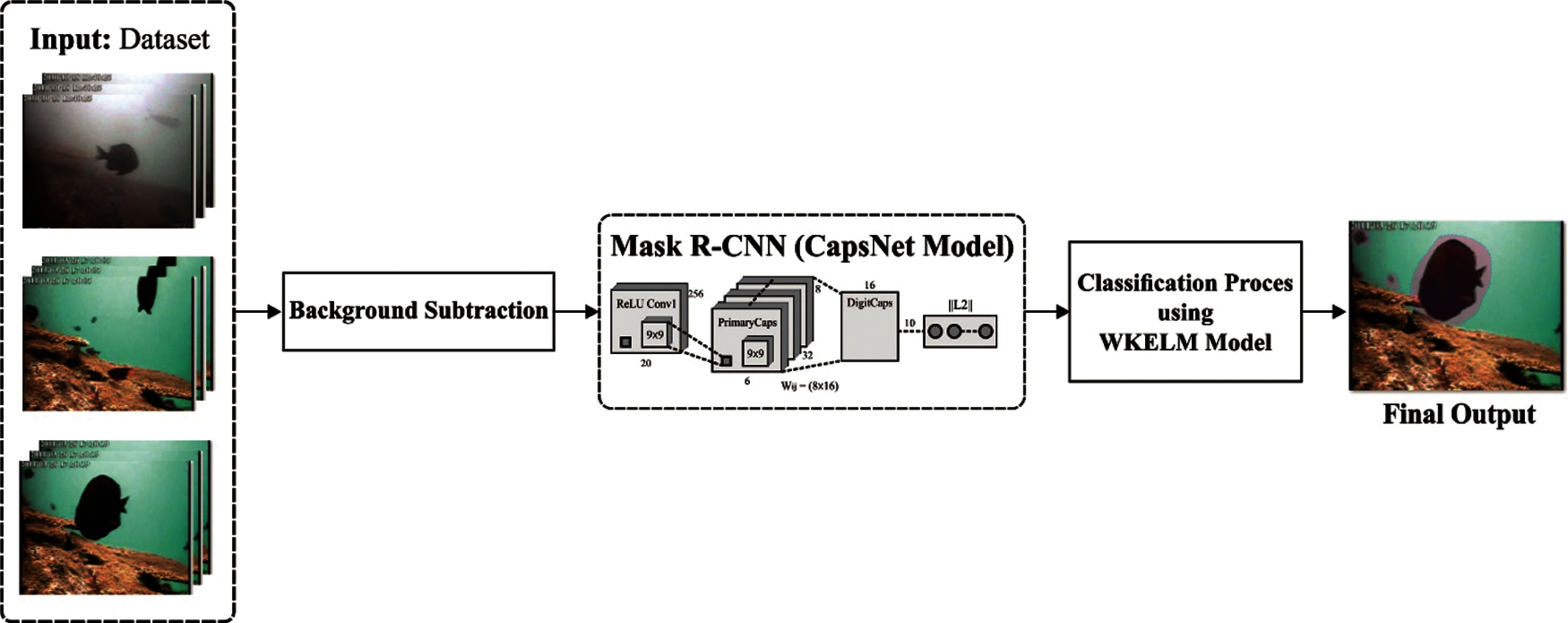
Figure 1: The overall working process of IDLAFD-UWSN model

4.1 Dataset Used

The presented model was tested using Fish4Knowledge with Complex Scenes (FCS) database. It is mainly created from a huge fish dataset known as Fish4Knowledge. With more than 700,000 underwater videos in unrestricted condition, the Fish4Knowledge database is a result of data collection for about 5 years that intended to monitor the marine ecosystem of coral reef in Taiwan [23]. It is a well-known area for large fish biodiversity environment in the globe with no less than 3,000 fish species. The database encompasses seven sets of elected videos, captured in standard underwater conditions with complex changeability in scenes. Thus, the ecological differences pose significant challenges to identify the fish as listed herewith.

•   Blurred, including three poor contrast blur videos.

•   Complex background includes three videos with rich seabed providing a maximum degree of backdrop confusion.

•   Crowded, in which a set of three videos is present with maximum density of fish movement in all video frames. This poses particular challenges to detect fishes under the existence of occluding objects.

•   Dynamic background, where two videos are given with rich texture of coral reefs backdrop and movable plants.

•   Luminosity variation includes two videos with abrupt luminosity variations, because of the surface wave action. It generates false positives during identification process, owing to the movement of light beam.

•   In Camouflage foreground, two videos are selected which show the camouflaging issue of fish detection in the existence of texture and colorful backdrop.

•   Hybrid, where a pair of videos is chosen to demonstrate the integration of previously-defined conditions of changeability.

This database is primary developed for fish-related tasks such as detection, classification, etc. So, the ground truth images exist for every moving fish on a frame-by-frame basis in every video. A set of 1,328 fish annotations is presented in FCS database as illustrated in Fig. 2.

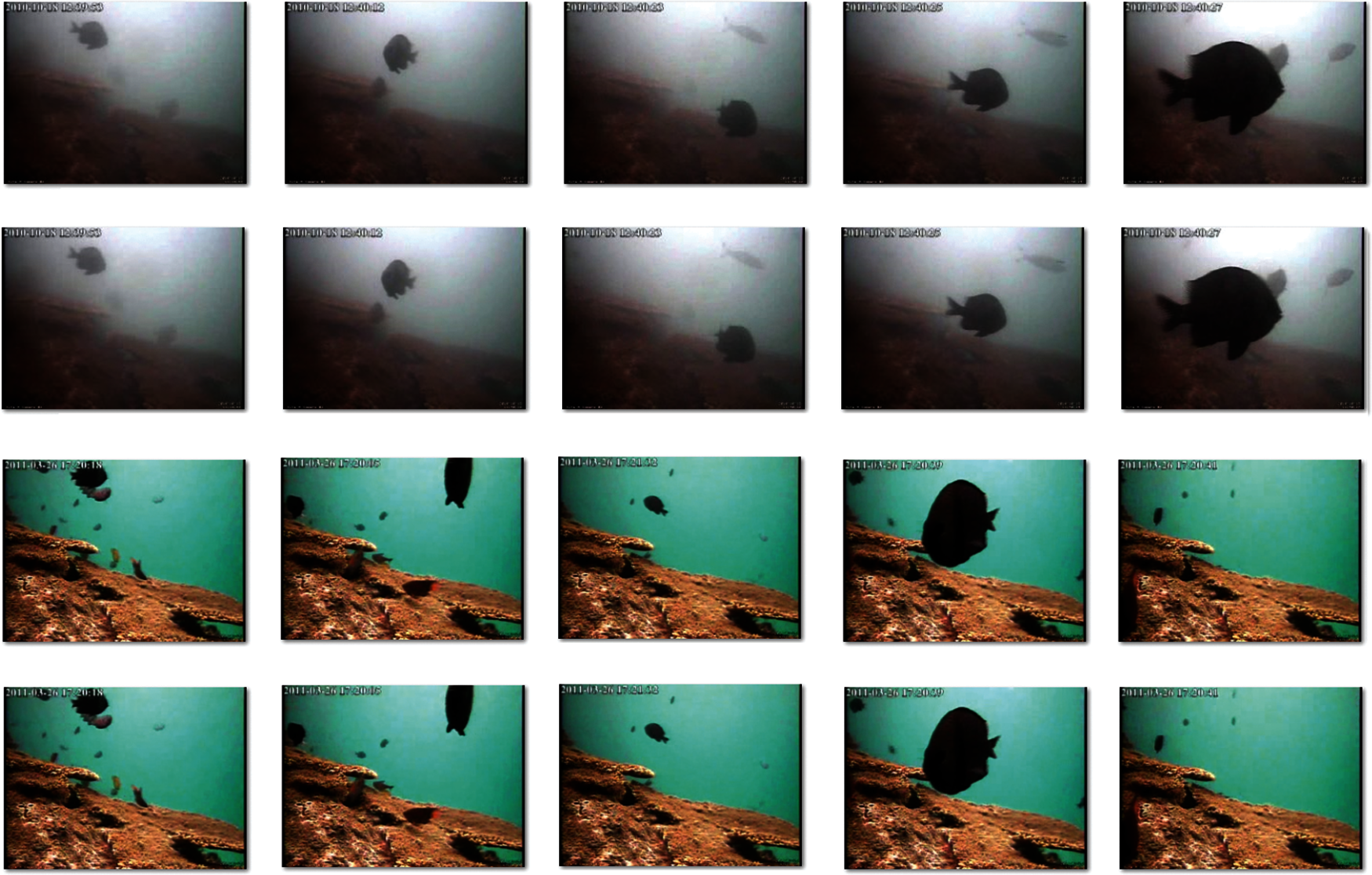
Figure 2: Sample test images from FCS database

4.2 GMM-Based Background Subtraction

GMM is one of the common methods used for modeling foreground and background conditions of the pixel. It has the capacity to perform general calculation as they could fit in all the density functions, when they possess sufficient combination. Here, It represents the frame of video t and p, the deliberate pixel coordinates (i,j)—and xtp denotes its RGB values in frame It. The instant values of this specific pixel, in time, are then implemented by:

{x1p,⋯,xtp}={It(i,j):1≤t≤T} (1)

where T denotes the counts of the frame. GMM is related to pixel p in RGB color space at frame t and it consists of K-weighted Gaussian function:

f(x)=∑k=1Kwk,tp.fg(x;μk,tp,Σk,tp) (2)

where K represents the amount of mode of combination, fg(x;μk,tp,Σk,tp): Gaussian density function of kth Gaussian mode of p in frame t,wk,tp represents the weight of mode k,μk,tp denotes the center vector and Σk,tp indicates the covariance matrix. Further, fg multivariate Gaussian function is shown herewith.

fg(x;μk,tp,Σk,tp)=1(2π)d|Σk,tp|exp−1/2(x−μk,tp)TΣk,tp−1(x−μk,tp) (3)

To simplify the estimation, covariance matrix is always considered as diagonal.

Σk,tp=σk,tp2I (4)

where I represents the identity matrix sized, 3×3.Thus, the R, G, B pixel levels are considered to be autonomous with equivalent difference. Though this might not be accurate, the statement avoids costly matrix inversion with regards to precision method.

4.2.1 GMM Initialization

This is an elective phase where the model employs EM (Expectation-Maximization) technique on a video portion; however, it could initiate an individual model for each pixel (of weight 1), that beings from the level of initial frame.

4.2.2 Mode Labeling

Every Gaussian mode is categorized as Background/Foreground. This crucial link is attained from a basic rule i.e., higher the precision and frequent modes, more possible to model the background colors [24]. Particularly, K modes are arranged based on their priority level, wkσk. The initial KB mode is later considered as background. The value of KB is defined by a threshold, Tb∈[0,1]:

KB=arg⁡min∑k=1Kwk,t>Tb (5)

4.2.3 Pixel Labeling

This step arranges the pixels. In all the techniques, a pixel is allocated to a class of nearest mode center in limitation.

‖xtp−μk,tp‖≤kpσk,tp (6)

where kp represents the constant coefficient which must be adjusted for every video. When no other modes fulfill this limitation, low priority mode is substituted by a novel Gaussian which is placed on the present intensity, xtp, with previous difference weights.

4.2.4 Updating GMM

An update function is given herewith.

When a mode i is efficaciously chosen, the GMM variables are then upgraded to reinforce this mode.

wi,t+1=(1−α)wi,t+α (7)

μi,t+1=(1−ρ)μi,t+ρ⋅xt+1p (8)

σi,t+12=(1−ρ)σi,t2+ρ‖xt+1p−μi,t+1‖2 (9)

∖wj,t+1=(1−α)wj,t,∀j≠j (10)

where α represents a constant learning rate and ρ=α.f(xt+1p,μi,σi).

Or else, the latter allocation is substituted by a novel Gaussian mode.

4.3 Mask RCNN Based Fish Detection

Mask R-CNN model is popular in several object detection tasks. It includes three components namely, CNN-based feature extraction, Region Proposal Network (RPN) and Parallel prediction network. At first, CNN model is applied in feature extraction from the input images. Secondly, RPN makes use of anchors under various scales and aspect ratios to glide on the feature maps so as to generate the generating region proposal. Thirdly, three branches from parallel prediction network with two FC layers are involved for bounding box classification and regression while FCN is involved to predict the object masks. Principally, baseline network is found to be a major model for Deep Neural Networks (DNN) namely, CapNet, GoogLeNet, and ResNet. In this study, MaskRCNN with CapsNet model are used whereas the CapsNet is utilized as the backbone network for feature extraction. This scenario results in effective reduction of gradient vanishing and reduced training with no increase in model parameters.

CapsNet method is one of the latest studies in this research domain. The key element of CapsNet is a capsule that comprises of a set of organized neurons. The length of capsule is decided based on invariance, whereas the number of features is present to reconstruct the image measurement of equivariance. The orientation of vector denotes its variables, i.e., data features are maintained in the image.

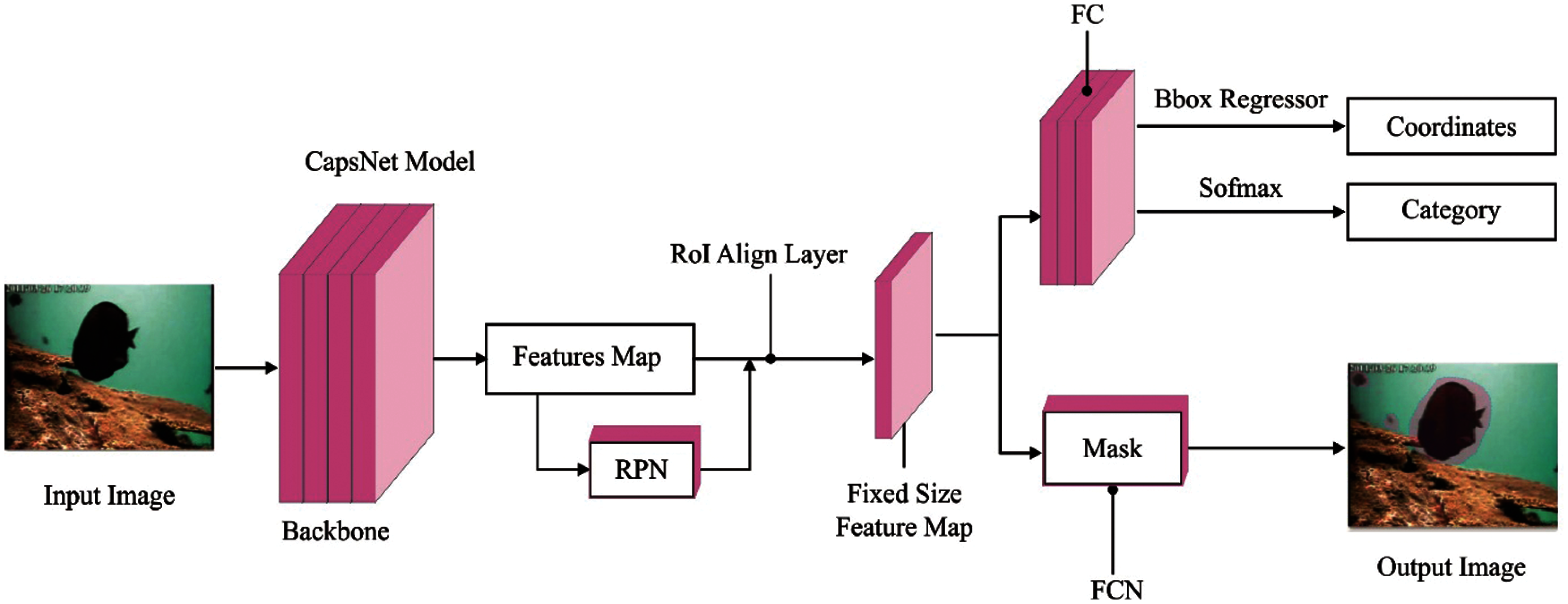
Figure 3: CapsNet process

When a standard NN requires extra layers to increase accuracy and details, with CapsNet, an individual layer can nest with other layers. The capsules efficiently denote distinct kinds of visual data which are known as instantiation variables and some of the examples are as follows integration of size, orientation, and position. Fig. 3 depicts the process involved in CapsNet model. The output of capsule represents the vector that could be transmitted to the above layer to match its suitable parent [25]. The output of capsule i is assumed to be ui whereas conversion matrix Wij is employed to capsule the output so as to predict the parent capsule j by converting ui to predict the vector U^j|i.

U^j|i=Wijui (11)

where U^j|i denotes the predictive vector of output of jth capsule in high level. This value is calculated by capsule i in below layer whereas Wij represents the weight matrix which should learn in backward pass. The variable sj denotes the weighted amount of entire set of predictive vectors uj|i. Here, cij represents the coupling coefficient, estimated by dynamic routing procedure that helps in the determination of degree of confirmation between the capsules in below layer and parent capsules. This connection is not designed by ‘max pooling’ of regular CNN. In contrast to max pooling, the entire details of the data are maintained. So, it increases the effectiveness by image overlapping. The dimension of capsules raises the hierarchy to ascend.

An activation function named ‘squashing’, shrinks the last output vector to 0, when it is smaller whereas when it is larger, it becomes unit vector and generates the capsule length. The activity vector vj can be estimated by succeeding nonlinear squashing function.

vj=||sj||21+sj||2sj||sj|| (12)

cij is calculated as softmax of bij. The coupling coefficient is determined by the degree of conformation between capsule and parent capsules.

cij=exp⁡(bij)∑kexp⁡(bik) (13)

bij represents similar scores considered for likeliness and characteristics, instead of likeliness in neurons.

bij=bij+U^j|ivj (14)

The primary network extracts low-level features such as edges whereas the upper network extracts the top-level features that denote the target class. In order to use the features effectively at every stage, Mask RCNN model extends the baseline network to Feature Pyramid Network (FPN). This network exploits both intrinsic layers and multi-scaling characteristics of CNN to derive meaningful features in the detection of objects. The aim of RPN lies in the prediction of set of region proposals in an effective way [26]. During RPN training, the anchor with maximum Intersection over Union (IoU) overlapping is used while the ground truth boxes are utilized as positive classes. Further, the anchor with IoU<0.3 are considered as negative classes. Here, IoU is determined as follows.

IoU=Detection Outcome ∩Ground TruthDetection Outcome ∪Ground Truth (15)

Here, detection outcome designates the predicted box and ground truth specifies the ground truth box. RPN fine-tunes the region proposals based on the attained regression details and discards the region proposals that overlap with image boundaries. At last, based on Non-Maximum Suppression (NMS), around 2000 proposal regions are kept for every image.

The region proposal, produced by RPNs, necessitates RoIAlign to adjust the dimensions for satisfying multibranch prediction network. RoIAlign utilizes bilinear interpolation rather than rounding function in RoIPool for faster R-CNN so as to extract the respective features of all-region proposals in feature map. When training the model, the loss function is determined for Mask RCNN model for all the proposals as given below.

L=Lcls+Lbox+Lmask, (16)

where Lcls, Lbox, and Lmask denote classification, regression, and segmentation losses; a definite computation of classification and regression losses is represented herewith.

Lcls+Lbox=1Ncls∑iLcls(pi,pi∗)+λ1Nbox∑iLbox(ti,ti∗), (17)

where i specifies the anchor index, pi signifies the predicted probability of anchor i, ti denotes four coordinate variables of the box, and ti∗ stands for coordinate variables of ground truth box with respect to positive anchor. When the anchor is positive, pi∗ becomes 1; else, pi∗ becomes 0. This technique can be optimized through minimization of loss function.

4.4 WKELM Based Classification

At this stage, WKELM model is applied to categorize the objects under fish or non-fish entities. WKELM model combines the benefits of distinct kernel functions and integrates the wavelet analysis with kernel extreme learning machine. The weighted ELM method is presented to manage the instances that are unbalanced in probabilities’ distribution while this technique acts excellent. Besides, the weighted WKELM technique establishes the weighted model-to-cost function so as to obtain the same result as weighted ELM [27]. KELM method derives from the ELM technique, and the weighted cost function is written as follows.

minLELM=C2‖β‖2+W2‖T---HV‖2 (18)

β={HT(CI+WHHT)−lWT,N<L(CI+HTWH)−lHTWT,N≥L (19)

In KELM method, the output is written as follows

y=[k(x→,x1→)k(x→,x2→)⋯k(x→,xN→)](CI+WKT)−lWT (20)

where K refers to kernel matrix, W implies the weighted matrix, and C denotes the regularization parameter.

5  Performance Validation

The experimental validation of the presented IDLAFD-UWSN model was performed with two testbeds from FCS dataset, namely, Blurred and Crowded. Both the testbeds comprised of a set of 5,756 frames with a duration of 3.83 minutes. Fig. 4 showcases the visualization images of IDLAFD-UWSN model.

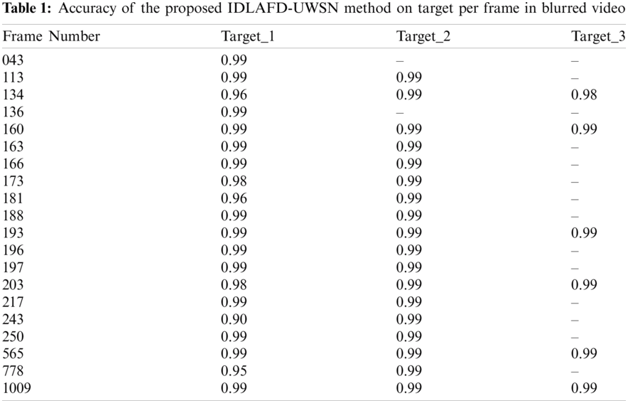
Tab. 1 shows the results for accuracy analysis of the proposed IDLAFD-UWSN model upon blurred video. From the figure, it is evident that the presented IDLAFD-UWSN model detects multiple targets effectively. For instance, on the test frame 134, IDLAFD-UWSN model detected targ_1, targ_2, and targ_3 with an accuracy of 0.96, 0.99, and 0.98 respectively. In addition, on the test frame 160, the presented IDLAFD-UWSN model detected the targets such as targ_1, targ_2, and targ_3 whereas its accuracy values were 0.99, 0.99, and 0.99 correspondingly. Moreover, on the test frame 173, IDLAFD-UWSN model detected targ_1 and targ_2 with an accuracy of 0.98 and 0.99 respectively. Also, on test frame 193, IDLAFD-UWSN model detected targ_1, targ_2, and targ_3 while its accuracy values being 0.99, 0.99, and 0.99 respectively. Additionally, on the test frame 203, IDLAFD-UWSN model detected targ_1, targ_2, and targ_3 with accuracy values such as 0.98, 0.99, and 0.99 correspondingly.

Figure 4: Visualization Images of IDLAFD-UWSN Model

Besides, on the test frame 565, the proposed IDLAFD-UWSN model achieved 0.99, 0.99, and 0.99 accuracy for the targets, targ_1, targ_2, and targ_3 respectively. In addition to the above, on the test frame 1009, IDLAFD-UWSN model found the targets such as targ_1, targ_2, and targ_3 while the accuracy values were 0.99, 0.99, and 0.99 respectively.

Tab. 2 shows the results of accuracy analysis attained by IDLAFD-UWSN model on crowded video testbed. From the figure, it is evident that the presented IDLAFD-UWSN model detected multiple targets effectively. For instance, on the test frame 019, the IDLAFD-UWSN model detected the targets such as targ_1, targ_2, targ_3, targ_4, targ_5, targ_6, targ_7, and targ_8 with an accuracy of 0.98, 0.98, 0.98, 0.98, 0.99, 0.98, 0.99, and 0.98 correspondingly. In the meantime, on the test frame 036, IDLAFD-UWSN model detected the targets such as targ_1, targ_2, targ_3, targ_4, and targ_5 while its accuracy values were 0.98, 0.87, 0.99, 0.96, and 0.99 correspondingly. At the same time, on the test frame 160, IDLAFD-UWSN model detected the targets such as targ_1, targ_2, targ_3, targ_4, and targ_5 with an accuracy of 0.96, 0.96, 0.99, 0.93, and 0.99 respectively.

Meanwhile, on the test frame 221, the proposed IDLAFD-UWSN model detected targ_1, targ_2, targ_3, and targ_4 while its accuracy values were 0.99, 0.95, 0.99, and 0.99 respectively. Afterwards, on the test frame 435, IDLAFD-UWSN model achieved the accuracy of 0.99, 0.78, and 0.97 for the targets, targ_1, targ_2, and targ_3 correspondingly. Followed by, on the test frame 1217, IDLAFD-UWSN model detected the targets such as targ_1, targ_2, targ_3, targ_4, targ_5, and targ_6 while its accuracy values were 0.99, 0.93, 0.96, 0.99, 0.99, and 0.99 correspondingly. Simultaneously, on the test frame 1506, IDLAFD-UWSN model detected the targets such as targ_1, targ_2, targ_3, targ_4, and targ_5 with an accuracy of 0.97, 0.99, 0.99, 0.99, and 0.99 respectively.

Tab. 3 shows an extensive comparison of the proposed IDLAFD-UWSN model against recent state-of-the-art techniques.

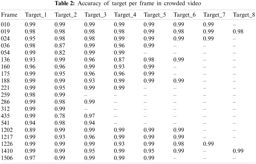
Fig. 5 shows the results of the accuracy analysis accomplished by IDLAFD-UWSN model and other existing methods on blurred and crowded testbeds. When analyzing the detection performance of IDLAFD-UWSN model in terms of accuracy on blurred video testbed, it is inferred that SCEA and ML-BKG models achieved ineffectual outcomes since its accuracy values were 71% and 72.94% correspondingly. Next, EIGEN technique attempted to attain slightly enhanced results with an accuracy of 82.89%, whereas FLDA, VIBE, and Hybrid system models demonstrated moderately closer accuracy values such as 86%, 86.35%, and 86.76% respectively. Simultaneously, FLDA-TM model exhibited a manageable performance with an accuracy of 88%. Though KDE and TKDE models showcased competitive results with its accuracy values being 91.73% and 93.78%, the presented IDLAFD-UWSN model accomplished the maximum accuracy of 98%. Similarly, when analyzing the detection performance of IDLAFD-UWSN model with respect to accuracy on crowded video testbed, it is inferred that SCEA and EIGEN models achieved ineffectual outcomes since its accuracy values were 70% and 75.82% correspondingly. Next, FLDA approach attempted to achieve somewhat improved outcomes with an accuracy of 80%. While, ML-BKG, Hybrid system, and KDE techniques exhibited moderately closer accuracy values such as 80.13%, 84.27%, and 84.83% respectively. Concurrently, VIBE model exhibited a manageable performance with an accuracy of 85.37%. Though TKDE and FLDA-TM models showcased competitive results with its accuracy values being 85.90% and 89%, the presented IDLAFD-UWSN model achieved the maximum accuracy of 97%.

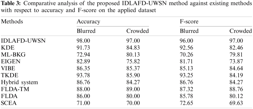
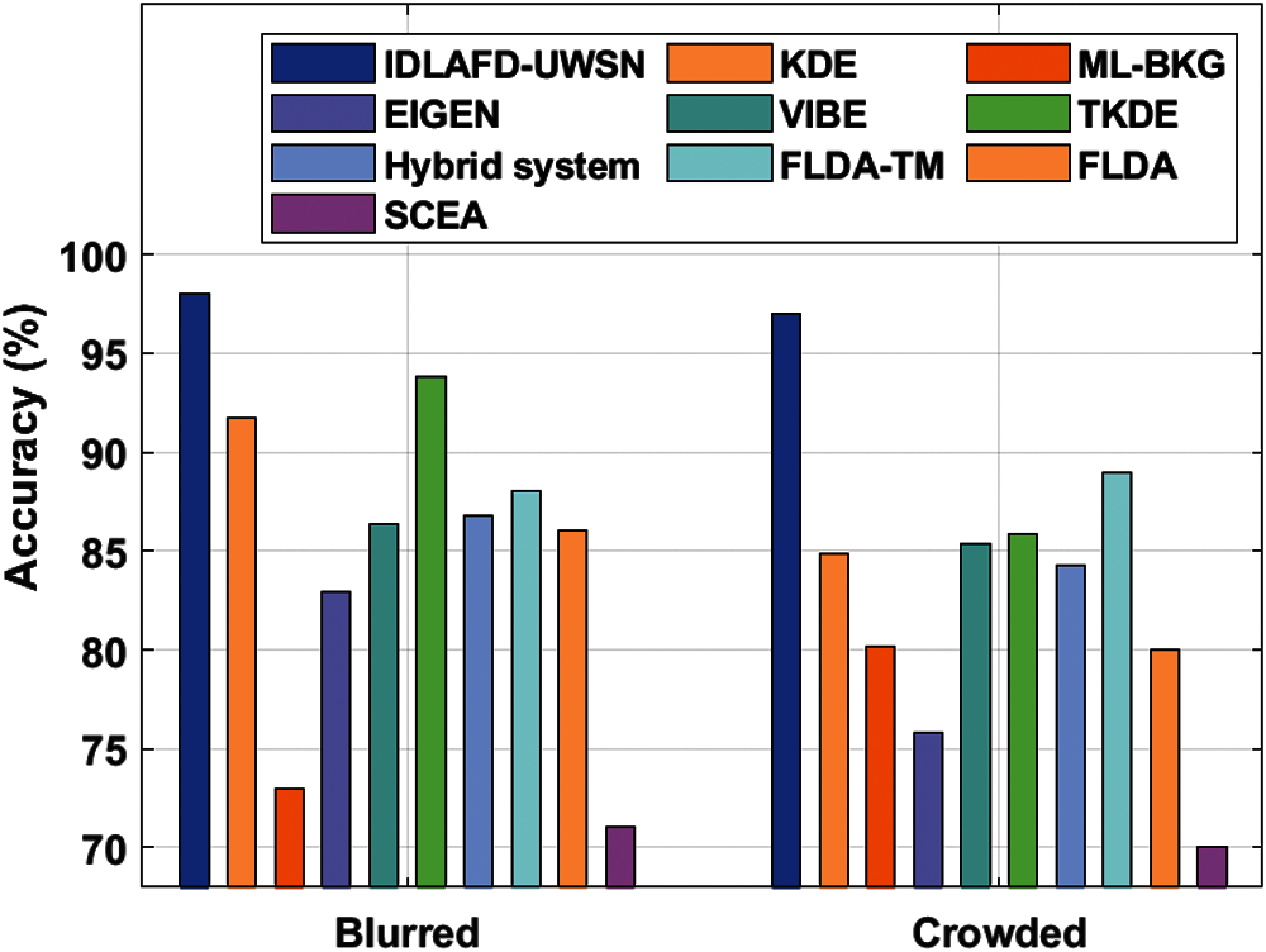
Figure 5: Accuracy analysis of IDLAFD-UWSN model against existing techniques

Fig. 6 examines the F-score analysis results achieved by IDLAFD-UWSN technique and existing models on blurred and crowded testbeds. When investigating the detection performance of IDLAFD-UWSN model with respect to F-score on blurred video, it is understood that ML-BKG and SCEA models achieved ineffectual outcomes with F-score values such as 70.26% and 72.65% respectively. Then, EIGEN model attempted to attain slightly enhanced results with an F-score of 81.71%, whereas VIBE, FLDA, and Hybrid system models demonstrated moderately closer F-score values being 85.13%, 85.78%, and 86.76% correspondingly. Similarly, FLDA-TM model exhibited a manageable performance with an F-score of 87.32%. Though KDE and TKDE models showcased competitive results i.e., F-score values such as 92.56% and 93.25%, the presented IDLAFD-UWSN model produced the maximum F-score of 98%.

Finally, when assessing the detection performance of the proposed IDLAFD-UWSN model in terms of F-score on crowded video testbed, the results conclude that SCEA and EIGEN models achieved ineffectual outcomes since its F-score values were 69.63% and 73.87% respectively. Afterward, ML-BKG model attained somewhat enhanced results with an F-score of 79.81%, whereas FLDA, KDE, and TKDE approaches demonstrated moderately-closer F-score values being 80.12%, 82.46%, and 84.19% respectively. At the same time, Hybrid system model exhibited a manageable performance with an F-score of 84.27%. VIBE and FLDA-TM models showcased competitive outcomes while its F-score values were 84.64% and 88.76%. The proposed IDLAFD-UWSN model outperformed all the existing models and produced the highest F-score of 97%.

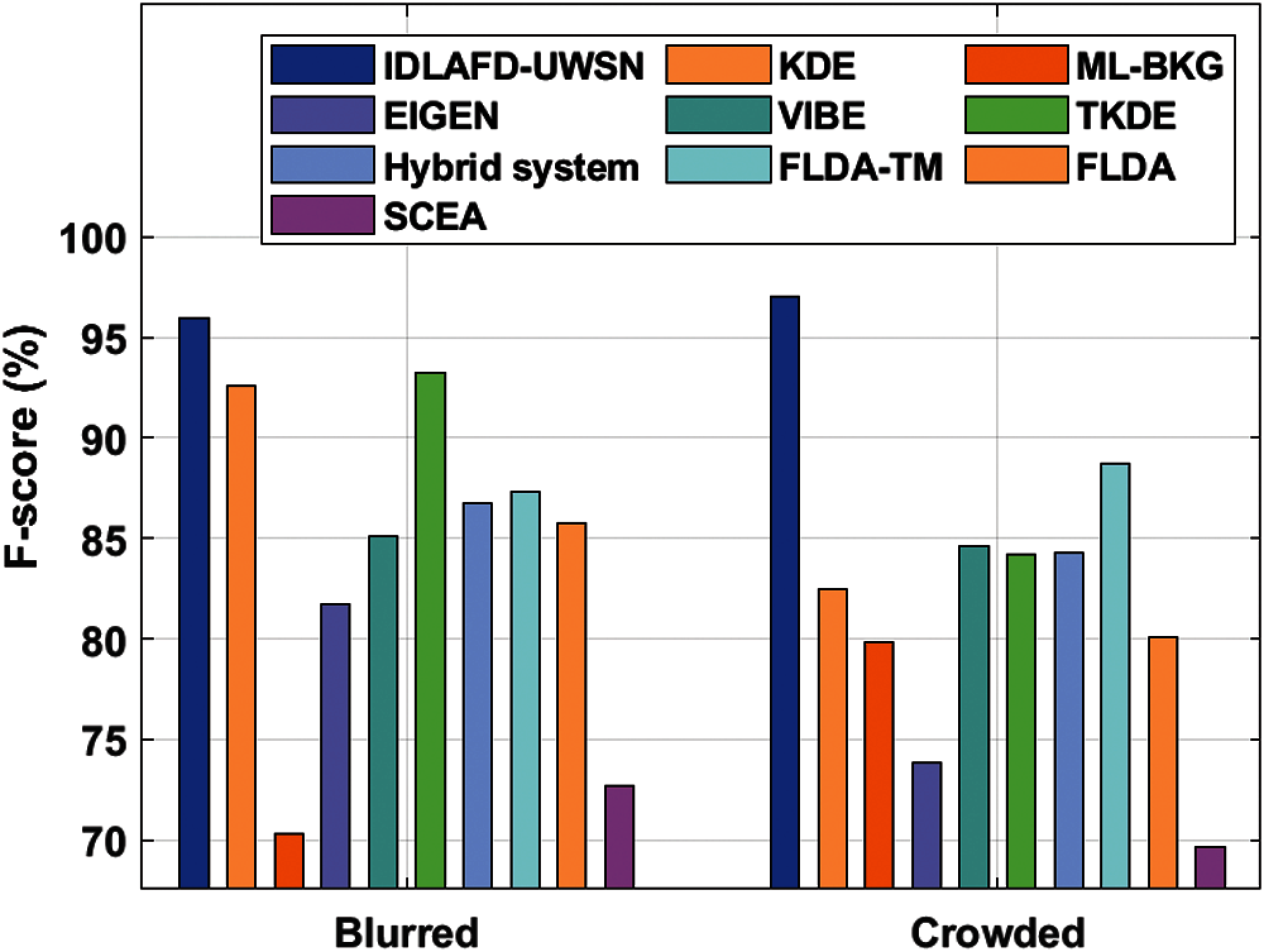
Figure 6: F-Score analysis of IDLAFD-UWSN model against existing techniques

From the above-discussed tables and figures, it is obvious that the presented IDLAFD-UWSN model accomplished promising results under blurred and crowded environments too. The improved performance is due to the inclusion of GMM-based background subtraction, MaskRCNN with CapsNet-based fish detection, and WKELM-based fish classification. Therefore, it can be employed as an effective fish detection tool in marine environment.

6  Conclusion

The current research article presented a novel IDLAFD-UWSN model for automated fish detection and classification in underwater environments. The presented IDLAFD-UWSN model aims at automatic detection of fishes from underwater videos, particularly in blurred and crowded environments. The presented IDLAFD-UWSN model operates on three stages namely, GMM-based background subtraction, MaskRCNN with CapsNet-based fish detection, and WKELM-based fish classification. MaskRCNN with CapsNet model distinguishes the candidate regions in video frame from fish to non-fish objects. Lastly, fish and non-fish objects are classified with the help of WKELM model. An extensive experimental analysis was conducted on benchmark dataset while the results of the analysis achieved by IDLAFD-UWSN model were promising with the maximum accuracy of 98% and 97% on the applied blurred and crowded datasets respectively. As a part of future extension, the presented IDLAFD-UWSN model can be implemented in real-time UWSN to automatically monitor the behavior of fishes and other aquatic creatures.

Funding Statement: The authors extend their appreciation to the Deanship of Scientific Research at King Khalid University for funding this work under grant number (RGP 1/53/42), www.kku.edu.sa. This research was funded by the Deanship of Scientific Research at Princess Nourah bint Abdulrahman University through the Fast-track Research Funding Program.

Conflicts of Interest: The authors declare that they have no conflicts of interest to report regarding the present study.

This work is licensed under a Creative Commons Attribution 4.0 International License, which permits unrestricted use, distribution, and reproduction in any medium, provided the original work is properly cited.