Computers, Materials & Continua DOI:10.32604/cmc.2022.021168
Article

Deep Neural Network Driven Automated Underwater Object Detection

Ajisha Mathias1, Samiappan Dhanalakshmi1,*, R. Kumar1 and R. Narayanamoorthi2

1Department of Electronics and Communication Engineering, SRM Institute of Science and Technology, Kattankulathur, Chennai, 603203, India
2Department of Electrical and Electronics Engineering, SRM Institute of Science and Technology, Kattankulathur, Chennai, 603203, India
*Corresponding Author: Samiappan Dhanalakshmi. Email: dhanalas@srmist.edu.in
Received: 25 June 2021; Accepted: 26 July 2021

Abstract: Object recognition and computer vision techniques for automated object identification are attracting marine biologist's interest as a quicker and easier tool for estimating the fish abundance in marine environments. However, the biggest problem posed by unrestricted aquatic imaging is low luminance, turbidity, background ambiguity, and context camouflage, which make traditional approaches rely on their efficiency due to inaccurate detection or elevated false-positive rates. To address these challenges, we suggest a systemic approach to merge visual features and Gaussian mixture models with You Only Look Once (YOLOv3) deep network, a coherent strategy for recognizing fish in challenging underwater images. As an image restoration phase, pre-processing based on diffraction correction is primarily applied to frames. The YOLOv3 based object recognition system is used to identify fish occurrences. The objects in the background that are camouflaged are often overlooked by the YOLOv3 model. A proposed Bi-dimensional Empirical Mode Decomposition (BEMD) algorithm, adapted by Gaussian mixture models, and integrating the results of YOLOv3 improves detection efficiency of the proposed automated underwater object detection method. The proposed approach was tested on four challenging video datasets, the Life Cross Language Evaluation Forum (CLEF) benchmark from the F4K data repository, the University of Western Australia (UWA) dataset, the bubble vision dataset and the DeepFish dataset. The accuracy for fish identification is 98.5 percent, 96.77 percent, 97.99 percent and 95.3 percent respectively for the various datasets which demonstrate the feasibility of our proposed automated underwater object detection method.

Keywords: Underwater images; diffraction correction; marine object recognition; gaussian mixture model; image restoration; YOLO

1  Introduction

Visual surveillance in underwater environments is grasping attention due to the immense resources beneath the water. The deployment of automated vehicles such as Automated Underwater Vehicles (AUV) and other sensor-based vehicles underwater is aimed to gain knowledge about the marine ecosystem. With the profound advancements in automation, the habitats in the ocean are watched by such automated remotely operated underwater vehicles. The knowledge about the fish abundance, endangered species, and their compositions are of great interest among ecological aspirants. Thus efficient object detection methods help in the study of the marine ecosystem. The underwater videos captured through Remotely Operated Vehicle (ROV) and submarines need to be interpreted to gain meaningful information. The manual interpretation is tedious with huge data loads, the automated interpretation of such data gain interest among the computer vision researchers. The major goal in underwater object detection is to discriminate fish or other ecological species from their backgrounds. The water properties lead to many geometric distortions and color deterioration which further challenges the detection schemes [1–5].

Various studies developed for underwater object detection helps in many ecological applications to a greater extent. The generic methods developed are useful in the detection of objects in challenging scenes. Yan et al. [6] introduced the concept of underwater object detection from the image sequence extracted from underwater videos based on statistical gradient coordinate model and Newton Raphson method to estimate the object position from the input underwater scenes. Vasamsetti et al. [7] developed an ADA-boost based optimization approach to detect underwater objects. The Ada-boost method is tested with grayscale images and detection is achieved based on edge information. Rout et al. [8] developed the Gaussian mixture model for underwater object detection which differentiates the background from the object of interest. Marini et al. [9] developed a real time fish tracking scheme from the OBSEA-EMSO testing-site. The tracking is based on K-fold validation strategy for better detection accuracy.

Automated systems prefer a faster convergence rate with large dataset processing. The advancements in machine learning help in automated detection for deployment in real-time applications. Li et al. [10] developed a template based machine learning scheme to identify fish and to classify them. The template method uses Support Vector Machines (SVM) for detection. The deep learning-based Faster Convolutional Neural Network (CNN) developed by Spampinato et al. [11], is efficient in object detection with faster detection rate yet the model is computationally complex. Lee et al. [12] developed a Spatial Pyramid Pooling model for its flexible windowing option in building object detection for improved detection accuracy. Yang et al. [13] implemented underwater object detection using YOLOv3, the faster convergence model. Jalal et al. [14] developed a classification scheme with hybrid YOLO structures to develop an automated detection scheme. The accuracy of YOLOv3 in .underwater frames are not satisfactory as in natural images.

From the literature, it is inferred that the deep learning algorithms such as CNN, Regions with CNN (RCNN) and Saptial Pryamid Pooling (SPP) are showing limited detection accuracy in challenging underwater environments. Out of these methods, YOLOv3 is one of the fastest. However, it cannot handle dynamic backgrounds well. Here arise the need for the development of an efficient underwater detection schemes that are suitable for challenging settings. The proposed automated underwater object detection framework includes

•   Data preprocessing phase by proposing an efficient diffraction correction scheme named diffraction limited image restoration (DLIR) to improve the geometric deteriorations of the input image frames.

•   In the second phase, the restored images are applied with the YOLOv3 model for fish detection of the challenging underwater frames.

•   In the third phase, a Bi-Dimensional Empirical Mode Decomposition (BEMD) based feature parameter estimation adapted to Gaussian Mixture Model (GMM) is proposed for foreground detection of an object. With the help of transfer learning, VGGNet-16, the GMM output is adapted as a neural network path, and the output is compared with YOLOv3 output for every frame to generate the output of the proposed automated object detection framework.

The article is organized as follows. Section 2 discusses about the proposed automated underwater object detection framework which includes the proposed Diffraction Limited Image Restoration, proposed Bi-dimensional Empirical Mode Decomposition adapted Gaussian Mixture Model and YOLOv3 based detection schemes. The experimentations, dataset descriptions, results and comparative analysis are presented in Section 3. Lastly the article is concluded in Section 4.

2  Proposed Automated Underwater Object Detection Scheme

The proposed automated underwater object detection approach is intended to detect multiple fish occurrences in underwater images. The frames retrieved from underwater videos constantly encounter issues of blurring, diffraction of illumination, occlusions and other deteriorations posing difficulties in object recognition. Thus for efficient detection of underwater objects the proposed detection scheme comprises of three modules. Fig. 1 represents the overall schematic of the proposed approach. The first data preprocessing module is intended in correcting the color deteriorations and geometric distortions in the input frames. The second module comprises of the BEMD based feature extraction for estimation of weight factor, texture strength and the Hurst calculation from the frames. The features are adapted with the generic GMM scheme for foreground object detection. The outcomes of GMM is provided to the transfer learning VGGNET-16 for generation of bounding boxes over the object of interest. In the third module, the pre-processed frame is feed to a YOLOv3 framework for object detection of the input underwater frames. By combining the outcomes of second and third module using an OR based combinational logic block, effective object detection is performed in underwater datasets.

Figure 1: Block schematic of proposed automated underwater object detection approach

2.1 Data Pre-Processing Using Proposed Diffraction Limited Image Restoration Approach

Underwater images need improvement for a variety of applications such as object detection, tracking, and other surveillances due to visibility degradations and geometric distortions. The Dark Channel Prior (DCP) approach [4,15] is the most commonly used method for restoring hazy or blurred images. The DCP method estimates the Background Light (BL) and Transmission Map (TM) for image restoration by calculating the depth map values of the red channel in the image. The DCP approach thus improves image clarity and colour adjustments while being limited in its ability to restore geometric deteriorations. For an effective underwater image restoration, the proposed diffraction limited image restoration scheme incorporates diffraction mapping along with DCP. The underwater image is primarily represented as

UI(x)=J(x)t(x)+BL(1−t(x))(1)

where UI(x) be the intensity of the input images at pixel x, J(x) is the original radiance of the object at pixel\; x, t(x) is the transmission map that differs mostly with color distribution of color in the three channels, and BL is the Background Light in the frame. The preservation of scene radiance J requires the analysis of the TM and BL.

The TM strength as illustrated by Beer-Lamberts law of atmospheric absorption as

t=e−βd(2)

which β is an exponentially decaying variable, whereas d denotes the range between the camera and the point of interest and is the illumination attenuation variable. The DCP method determines the least possible intensity value of an image patch\; Ω(x). The color image's DCP represented as

UIdcp(x)=y∈Ω(x)min{minUI(y)}(3)

The BL value is estimated as

BL=brightestpixelargmin∑⁡UI(x)×UI(4)

For clear scene outcomes, the TM will be near unity and hence the UI approximated to be close to J(UI≅J). The TM according to DCP is thus estimated as

t(x)=1−y∈Ω(x)min{minUI(y)BL}(5)

For the proposed diffraction limited restoration is shown in Fig. 2. The selected underwater frame is applied with basic quad-tree division. The quad-tree division simply divides the image into four equal segments. For every segment, the intensities of every pixel need to be calculated. The segment which holds the maximum intensity is chosen as the latent patch U with size\; h×h. Let R be the entire region of the input frame and x be the pixel in any ith instance. Let h be the limiting or degrading factor that can be considered as point spread function (PSF). Let J be the scene clarity desired to be restored as the actual image. As per the diffraction theory, the image model can be expressed as

Ui=x⊗fi⊗j+ηi(6)

Figure 2: Block schematic of proposed diffraction limited image restoration approach

Considering the shifted PSF variable to be fi^ and position changing noise function as\; ηi^.

Ui=x⊗j⊗f^i+η^i=Qi+η^i(7)

where Qi=x⊗j,\; be the limiting factor in terms of diffraction in the ith frame. Regression functions are known to limit the degradation by using a kernel function. The cost function of the kernel regression function is\; W(q;i,μk), where μk the Kernel Regression Function, and it is always remain constant. The kernel weight variable applied to the entire patch be,

Qi=(∑i⁡Ui(q)W(q;i,μk))/∑iW(q;i,μk)(8)

The degradation factor of the selected patch Ui at the pixel position q is expressed by the kernel regression Fi. Let the cost function is W(q;i,μk)=exp(−ΔF2(μkh)2). The new diffraction corrected reconstruction with the least degradation is given as

Di(q)=∑i⁡αiUi(q)=αTi[q](9)

αi is the random weight coefficients in which α is a vector that ranges from α1,α2,…,αi  and  i1[q] is the corresponding pixel constant, and i is the direction coordinate that ranges fromi1[q],i2[q],..ii[q]. The weighted cost function is argminα∑iϵq⁡W||Qq−Qi||2+λ||α||2, λ is the regularization factor, is always a positive factor. The optimization of diffraction-limited reconstruction is given by,

argminϕα=λ||α||2+∑i∈q⁡Wi||Di(q)−i[q]||2+2σ2ΔQi−σ2(10)

where σ2, corresponds to the variance of noise factor. After decreasing and trying to conflate the weights, the regularization function generates a linear model, as

α=(A+λj)−1dk,dk=∑⁡i∈q(11)

The restored image U\; was created by fusing all of the patches for the whole area\; R. Underwater image reconstruction was done by approximating the average propagation chart and the distribution of background light. The DCP approach makes an effort to approximate the TM and BL. The intensity value in the red channel was calculated as

UR(x)=maxy∈Ω(x)UIr(y)(12)

By means of Eqs. (3)–(4), the TM and BL are evaluated, and the restoration is accomplished by rewriting Eq. (1) as

J(x)=1t(x)(I(x)−BL)+BL(13)

The obtained actual output J is the restored image of the proposed diffraction limited restoration method as a data preprocessing stage will be the input for the subsequent detection frame works.

2.2 Proposed BEMD-GMM Transfer Learning Module

The object detection technique is primarily used to recognize objects in an image and identify their position. If one or more objects exist the detection scheme evaluates the existence of multiple objects in the frame with bounding boxes. The challenging underwater scenes need efficient detection scheme to detect blurred and camouflaged objects in the image.

To perform effective underwater object detection, a Bi-dimensional Empirical Mode Decomposition based Adaptive GMM scheme (BEMD-GMM) is proposed. Object detection can also called as background subtraction is depend profoundly on image intensity variance. The image intensity variance of the images can be viewed more easily in the frequency domain. BEMD is a non-linear and non-stationary version for 2D image decomposition proposed by Nunes et al. [16]. The BEMD is a variant of the widely used Hilbert–Huang Transform (HHT) which decomposes the 1D signals. The preprocessed image frames are subjected to BEMD algorithm for intrinsic mode decompositions. The various modes are iteratively generated until a threshold is reached. The weight factor, texture strength, and Hurst Exponent are retrieved from the residual Intrinsic Mode Function (IMF) as feature for the blob synthesis. These features acts as the reference for GMM model for object detection. The sifting procedure for BEMD algorithm is represented in Fig. 3. In the figure, the input frame is decomposed with possible IMFs and the features are extracted. Any 2D signal can be decomposed into multiple IMF's. The input image is decomposed into the biaxial IMF during the sifting process. The following are the phases in the sifting of 2D files. The procedure is begun by setting the residual function to the same value as the input.

res(k,l)=Y(k,l)(14)

where Y(k,l) is the input image with k and l as the co-ordinates. For the measurement of maxima and minima pixels, the minimum intensity pixel and maximum intensity pixel are defined. Interpolating the minima and maxima points yields the lower bound of the envelope value, denoted as El(k,l), and the upper bound of the envelope value, denoted as Eu(k,l). The envelope mean value is computed as

ME(k,l)=(El(k,l)+Eu(k,l))/2(15)

Figure 3: Proposed Bi-dimensional empirical mode decomposition on underwater images with residual outcomes and their corresponding surf plot and hurst calculation

The IMF number is determined by the modulus of the above mean value.

Mod(k,l)=res(k,l)−ME(k,l)(16)

The procedure is iterative until the stopping criteria is satisfied. The stopping criteria is

res(k,l)≅Mod(k,l)(17)

The precision value derived from the BEMD morphological reconstruction is the weighted cost function. The three extrema precision values correspond to the IMF's: 0.00000003, 0.00003, and 0.03. It is necessary to perform fractal analysis on BEMD results, which requires the calculation of the Hurst Exponent and texture strength. Hurst exponent is the relative index of the dependence of the self-IMF. This measures the regression of time series data for them to converge to their corresponding mean values as

E{K(n)δ(n)}=CH;n→∞(18)

where K(n) is the range factor of the first derivative mean; δ(n) is the standard deviation; E{K(n)δ(n)} is the expected coefficient; H is the Hurst exponent; n is the quantity of time-series data points and C is the constant. The predicted coefficient is fitted to the power law and plotted to approximate the H as log[K(n)δ(n)] as a function of log⁡n to fit into a straight line. The slope denotes the Hurst ExponentH. TheH value with 0.5 or greater carries meaningful information. H usually ranges from 0.1 to 0.9. Texture strength is derived from the decomposed IMF of BEMD by taking the log of covariance. The blob selection is done the integrating the precision weight(ω), texture strength (τ),and Hurst exponentH. The Hurst exponent is a valuable method for creating blobs in complicated scenes. This is due to the exponent being set to 0.5 or greater. The effective cost function is calculated as

Ki=a×ωi+b×τi+c×H(19)

where a,bandc are attributes to maintain the K-blob variable as a positive function. The target location is thus calculated as

St=∑i=1N⁡ki^{st^}(20)

where St is the new object position and st is the featured particles. Before the residual value reaches its limit, the image is decomposed into a set of Intrinsic Mode Functions (IMF). This IMF is plotted in 3D to see if the higher frequency parts decompose in the resulting IMFs. The Hurst plot is mapped against log (mean) to log (variance), and the slope score is considered as the Hurst exponent. GMM based detection is one of the shape, texture, and contours feature-based object detection schemes. Here, the entire distribution of data is considered as a Gaussian function. The bell-shaped Gaussian profile is close to a normal distribution function. The clustering of each Gaussian distribution profile is collectively termed as a Gaussian Mixture Model. The mean and variance of a Gaussian distribution function are usually calculated using maximum likelihood approximation. The GMM for multivariate system is expressed as

N(x|μ,Σ)=12π|Σ|1/2exp{−12(x−μ)TΣ−1(x−μ)}(21)

where μ is the mean and ε is the co-variance. The GMM method models the image based on the calculated weight factor, texture strength and Hurst exponent. The blobs are generated from the BEMD parameters and the detected objects are exposed as a bounding box. The estimated foreground information is fed as input to the VGGNet-16 (Visual Geometry Group Net) transfer learning model. VGGNet is a traditional neural network scheme created by Oxford University for large-scale visual recognition [17]. In the proposed framework, the VGGNet is preferred over complex architectures because feature blobs generated by GMM models must be transferred to the network. Advanced architectures want the network to extract features from the input image, which is not relevant in the proposed approach. The VGGNet used here has 16 layers, including a convolutional layer, a pooling layer, and a fully linked layer. During training, the input to VGGNet is an RGB image with a fixed size of 224 × 224. The image goes through a pile of convolutional layers using modified filters. The small detection area chosen is 3 × 3. Linear transformation of the input channel spatial padding is fixed with the resolution of each pixel. This architecture adapts the feature of foreground object estimated by the generic GMM detection scheme. Let the features used to perform foreground detection be considered as x. The new domain F of the transfer learning model thus includes the feature vector x along with its marginal probability, sayP(x).

F={x,P(X)}(22)

where X={x1,…,xn}xi∈X. To perform any operation using the gained feature knowledgex, the detection is performed as

D={y,P(Y|X)={y,φ}(23)

As the name indicates, the VGGNet-16 transfers the feature ideology of GMM and generate output to adapt the deep learning domain for further stages. The proposed BEMD-GMM method exhibits more clarified detection of camouflaged objects with dynamic environments. The convergence is moderate and the detection of blurred and occluded objects other than standard objects is limited in challenging underwater conditions.

2.3 YOLOv3 Object Detection for Challenging Underwater Scenes

The significance of the YOLO model is its high detection speed. The features extracted and trained from the training dataset are fed into the YOLOv3 model's input data. The YOLOv3 incorporates a DARKNET-based feature extraction scheme comprised of 53 convolutional neural layers, each with its own batch normalization model. The architecture of YOLOv3 is shown in Fig. 4. This network provides candidate detection boxes in three different scale. The offset of bounding box considers the feature maps 52 × 52, 26 × 26, and 13 × 13. The higher order feature maps are used in multiclass detection applications. To resist the vanishing gradient problem, the activation function is leaky ReLU (Rectified Linear Units).

Figure 4: Schematic of YOLO v3 network

3  Experimental Results and Discussion

The proposed automated underwater object detection scheme is tested with various challenging scenes categorized as normal scenes, occluded scenes, blurred scenes, and dynamic scenes. The experiment is carried out with an Intel®CorTMe-i7 CPU, 16 GB RAM, and an NVIDIA GeForce GTX 1080 Ti GPU. The Tensor Flow deep learning libraries for YOLO are used, while GMM and BEMD are performed in MATLAB 2020b. The YOLO hyper parameters are initialized with the primary learning rate as 0.00001 and as the number of epoch's increases the learning rate is reduced to 0.01. Once the image frame is read by the YOLOv3, it is processed by the blobFromImage function to construct an input blob to feed to the hidden layers of the network. The pixels in the frames are scaled to fit the model ranging from 0 to 1. The generated new blob now gets transferred to the forward layers for prediction of bounding box as the output. The layers concatenate the values and filter the low confidence scoring entities. The bounding box generated is processed with non-maximum suppression approach. This reduces the redundant boxes and checks for threshold of confidence score. The threshold needs appropriate range fixing for proper detection outputs. The NM filters are set to a minimum threshold of 0.1 in YOLOv3 applications. In underwater applications, due to the challenges in water medium, high confidence score is preferred for even moderate detection accuracy. If the threshold is high as close to 1, it leads to generation of multiple bounding boxes for a single object. The threshold is set to 0.4 in our experiments for appropriate box generation. The runtime parameters are shown in Tab. 1.

3.1 Dataset Details

The proposed method is tested with four challenging datasets to illustrate the feasibility of our proposed methodology. The first dataset is from the Life CLEF 2015, and it comprises 93 annotated videos representing occurrences of 15 different fish breeds. The frame resolution is 640 × 480. This dataset was obtained from Fish4Knowledge, a broader archive of underwater images [18]. The second dataset is gathered and provided by the University of Western Australia (UWA) which comprises 4418 video sequences of frame resolution 1920 × 1080 [19]. Among these, around 2180 frames are used as training frames and 1020 frames are subjected to testing. The third dataset is from the Bali diving dataset with a resolution of 1280 × 720 for output comparison [20]. The challenging dataset DeepFish [21] developed by Bradley and his teammates in from the coastal marine beds of tropical Australia is also tested. The dataset comprises of 38,000 diverse underwater scenes which includes coral reefs and other marine organism. The resolution is of 1920 × 1080 among which 30% (10,889 scenes approximately) is validated and tested in the proposed approach.

3.2 Diffraction Correction Results

The analysis of underwater images was subjected to numerous tests to determine the feasibility of the proposed approach. The proposed technique is compared to previous approaches such as DCP [22], MIL [23], and Blurriness Correction (BC) [24]. The simulation experiment measures the algorithm's efficiency. Several difficult illustrations of underwater scenes are chosen for the simulation. The test was performed with BL values of (0.44, 0.68, 0.87) for visually blue looking images, (0.03, 0.02, 0.2) for red and dark looking images, and (0.14, 0.85, 0.26) for greenish images. The majority of the red-spread frames are dark. The transmitting maps for red, blue, and green are 0.2, 04, and 0.8, accordingly. The DLIR methods performance is validated with the full reference metrics including Peak Signal to Noise Ratio (PSNR), Mean Square Error (MSE), Structural Similarity Index Metrics (SSIM), and Edge Preservation Index.

DLIR outputs of underwater images of different luminous scenes are shown in Fig. 5. The increased range of PSNR value exposes the improved quality of the restored image. The MSE should be as low as possible so the error factor must be as low as possible to achieve better reconstruction. The SSIM value should be close as unity for better restoration which exhibits lesser deviation from the original. EPI is Edge Preservation Index which also needs to be close as unity for better conservation of restored output. Tab. 2 relates different algorithms to the proposed approach quantitatively. The simulation is run with a frame size of 720 × 1280. The time taken for pre-processing using DLIR method is 0.6592 s, indicating that the algorithm has less computational complexity than many current algorithms.

3.3 Proposed Automated Object Detection Analysis

The object detection efficiency of the proposed method is tested and the results of varying scenes are analyzed qualitatively. Fig. 6 represents the detection outcomes of the proposed method with the frames from Life CLEF-15, UWA, and Bubble vision dataset. The shape and size of the bounding box varies following the shape and size of the object of interest. From the detection outcomes, it is observed that the GMM output detects the camouflaged object in clip 132 and the blurred objects in clip 122 and missed the object in clip 48. It is also visualized that the YOLOv3 output can detect the blurred object in clip 48. Thus at the combined output of the proposed, the objects are detected as the joint contribution of the GMM method and YOLOv3 method.

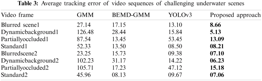
Fig. 6 demonstrates the object detection of complex underwater scenes, collectively referred to as DeepFish. The results distinguishes between object identification pre and post underwater image restoration. The output clearly shows that the DLIR restored frames helps in better detection than the actual input image. Furthermore, the BEMD-GMM model outperforms the YOLOv3 approach because it is more sensitive to occluded and dynamic scenes. The proposed automated detection scheme misses a few instances that are even more difficult to determine. As shown in image 4, 1763 images out of 38,000 images of the DeepFish dataset missed the detection. The proposed approach is tested for its validation in terms of Average Tracking Error (ATE) and IOU and is compared with the existing GMM, BEMD-GMM, Yolov3 algorithms. Tab. 3 shows the average tracking error of various methods. The ground truth values are calculated manually by considering the width and height of the object of interest and its centroid position.

Figure 5: Diffraction correction of underwater images based on the proposed pre-processing scheme taken from bubble vision video [20]. (a) Input frame, (b) Corresponds to the h × h latent patch, (c) Diffraction correction in X and Y direction, (d) Diffraction corrected image, (e) Depth map estimation, (f) Transmission map estimation and (g) Proposed diffraction corrected output

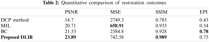
Figure 6: Object detection outcomes of original underwater images and the restored images of deepfish dataset [21]. (a) Represents the input challenging scenes and their restored images (b) Represents ground truth (c) Represents detection based on BEMD-GMM approach (d) Represents the detection based on YOLOv3 approach and (e) Represents the proposed automated object detection approach

Extensive evaluation of the proposed scheme is performed and the metrics including accuracy of detection, recall, the precision of tracking, and speed of detection (Fps) are calculated to gauge the proposed method. The metrics are estimated by calculating the True Positive (TP), False Positive (FP), and False Negative (FN) detection constraints. The speed of detection is measured as 18 Fps (Frames per second) whereas the conventional YOLOv3 model can detect 20 Fps since the architecture is simple than the proposed scheme. The results are compared with the state-of-art deep learning schemes of underwater object recognition including SVM [25], KNN [26], CNN-SVM [11], CNN-KNN [12], and YOLOv3 [13] schemes. The performance analysis is shown for the LCF-15 dataset, UWA dataset, Bubble Vision dataset and the DeepFish dataset in Fig. 7. The accuracy for fish identification is 98.5 percent, 96.77 percent, 97.99 percent and 95.3 percent respectively for the different datasets which validate the efficacy of the proposed method.

Figure 7: Performance evaluation of the proposed detection scheme in comparison to the SVM, KNN, CNN-SVM, CNN-KNN, and YOLOv3 models for various datasets

The IoU metric is a metric to determine the correctness of bounding box positioning in object detection approaches. The value of IoU ranges from 0.1 to 1.0 which precisely means, if the IoU metric reads above 0.5, the prediction is valid. As the name indicates the ratio of the area of intersection over the area of union is the IoU is estimated for the input sequences. From the IoU outcomes in Fig. 8, it is evident that the convergence of output of the proposed scheme is around 0.8 and it is close to unity and this shows the correctness in object detection.

Figure 8: IoU measure of the proposed method concerning the ground-truth value. The red box represents the proposed algorithm and green defines the ground truth

4  Conclusion

Efficient object recognition has been the key goal in underwater object detection schemes. In this article, we have developed and demonstrated an automated underwater object detection framework that performs object detection of challenging underwater scenes. The output of the proposed automated detection scheme is gauged for its precision in terms of reduced tracking error than the earlier available detection schemes. The proposed detection scheme can be used in underwater vehicles equipped with high-end processors as an automated module for detecting object of interest by marine scientists. As the proposed method is particularly developed for challenging underwater scenes, the method is efficient in detection of occluded and camouflaged scenes. Although the approach shows improved detection accuracy from the existing schemes, the work is still limited in the detection of objects from highly deteriorated scenes. Future work includes developing efficient tracking algorithms for ecological classification applications and developing more tracking trajectories for features derived from the objects.

Funding Statement: The authors received no specific funding for this study.

Conflicts of Interest: The authors declare that they have no conflicts of interest to report regarding the present study.

This work is licensed under a Creative Commons Attribution 4.0 International License, which permits unrestricted use, distribution, and reproduction in any medium, provided the original work is properly cited.