Computers, Materials & Continua DOI:10.32604/cmc.2022.021299
Article

Artificial Intelligence Enabled Apple Leaf Disease Classification for Precision Agriculture

Fahd N. Al-Wesabi1,2,*, Amani Abdulrahman Albraikan3, Anwer Mustafa Hilal4, Majdy M. Eltahir1, Manar Ahmed Hamza4 and Abu Sarwar Zamani4

1Department of Computer Science, King Khalid University, Muhayel Aseer, Saudi Arabia
2Faculty of Computer and IT, Sana'a University, Yemen
3Department of Information Systems, College of Computer and Information Sciences, Princess Nourah Bint Abdulrahman University, Saudi Arabia
4Department of Computer and Self Development, Preparatory Year Deanship, Prince Sattam bin Abdulaziz University, Alkharj, Saudi Arabia
*Corresponding Author: Fahd N. Al-Wesabi. Email: falwesabi@kku.edu.sa
Received: 28 June 2021; Accepted: 29 July 2021

Abstract: Precision agriculture enables the recent technological advancements in farming sector to observe, measure, and analyze the requirements of individual fields and crops. The recent developments of computer vision and artificial intelligence (AI) techniques find a way for effective detection of plants, diseases, weeds, pests, etc. On the other hand, the detection of plant diseases, particularly apple leaf diseases using AI techniques can improve productivity and reduce crop loss. Besides, earlier and precise apple leaf disease detection can minimize the spread of the disease. Earlier works make use of traditional image processing techniques which cannot assure high detection rate on apple leaf diseases. With this motivation, this paper introduces a novel AI enabled apple leaf disease classification (AIE-ALDC) technique for precision agriculture. The proposed AIE-ALDC technique involves orientation based data augmentation and Gaussian filtering based noise removal processes. In addition, the AIE-ALDC technique includes a Capsule Network (CapsNet) based feature extractor to generate a helpful set of feature vectors. Moreover, water wave optimization (WWO) technique is employed as a hyperparameter optimizer of the CapsNet model. Finally, bidirectional long short term memory (BiLSTM) model is used as a classifier to determine the appropriate class labels of the apple leaf images. The design of AIE-ALDC technique incorporating the WWO based CapsNet model with BiLSTM classifier shows the novelty of the work. A wide range of experiments was performed to showcase the supremacy of the AIE-ALDC technique. The experimental results demonstrate the promising performance of the AIE-ALDC technique over the recent state of art methods.

Keywords: Artificial intelligence; apple leaf; plant disease; precision agriculture; deep learning; data augmentation

1  Introduction

Plant phenotyping and Precision agriculture are information and technology based domain with certain challenges and demands for the detection and diagnoses of plant diseases [1]. This scheme's aim is to achieve real world, strong mapping system for environment, crop, and soil parameters for facilitating a management decision [2]. In contrast, conventional agricultural management practice assumes that parameters in crop fields are homogeneous, thus leads to crop health management and pesticide application that isn't obviously interrelated to the current disease management condition. Enhancing agriculture productivity needs advanced solution which provides improved quality and yield for outdoor and indoor farming [3]. A farmer requires precision technique for obtaining and interpreting the data for well controlled crop development, avoiding losses created by adverse climate conditions/infectious pests, and therefore enabling return on investment [3]. Yearly, plant disease contributes to substantial damages in global harvest, costing an estimated US$220 billion. Plant disease evaluation is accompanied for analyzing the measurement of pathogens or disease (phythopathometry), that is essential for estimating the crop loss and disease intensity. Abundant usage of chemicals like nematicides, bactericides, and fungicides for controlling plant diseases is created adverse impacts on several agroecosystems. A reliable and accurate method is required in plant disease evaluation for increasing severity estimation plant and disease detection.

Traditionally, visual observation by professionals was accompanied for diagnosing plant diseases. But, there is a threat for error because of subjective perceptions [4]. Regarding this, several spectroscopic and imaging methods were investigated to detect plant disease. Though, they need accurate bulky sensors and instruments that lead to higher costs and lower performance. Recently, using the popularisation of digital cameras and another electronic device, automated plant disease diagnoses through ML were broadly employed as suitable alternative [5]. ML methods are highly suitable for the detection of uniform background plant images that were taken in an ideal laboratory platform. In recent times, DL and convolutional networks have created significant developments in computer vision and several related practical and theoretical attainments have been stated [6]. Since CNNs could extract features directly and automatically from the input images, thus evading complicated preprocessing on images, they have been a study in object identification. But, executing the real world recognition of apple leaf disease remains complex due to ALDD has the succeeding features: firstly, many diseases might occur on similar leaves [7]. Additionally, all the spots of apple leaf disease are tiny. Lastly, environmental aspects like soil, shadow, and illumination also affect by apple leaf disease detections.

This paper introduces a novel AI enabled apple leaf disease classification (AIE-ALDC) technique for precision agriculture. The proposed AIE-ALDC technique encompasses orientation based augmentation, Gaussian filtering (GF) based noise removal processes. In addition, the AIE-ALDC technique includes a Capsule Network (CapsNet) based feature extractor to generate a helpful group of feature vectors. Moreover, water wave optimization (WWO) technique is employed as a hyperparameter optimizer of the CapsNet model. Finally, bidirectional long short term memory (BiLSTM) model is used as a classifier to determine the appropriate class labels of the apple leaf images. A wide range of experiments was carried out to showcase the supremacy of the AIE-ALDC technique.

The paper organization is given as follows. Section 2 offers the related works, Section 3 elaborates the proposed model, Section 4 provides the performance validation, and Section 5 concludes the paper.

2  Related Works

Liu et al. [8] presented the accurate detecting technique for apple leaf diseases on the basis of DCNN. It consists of creating adequate pathological images and design a new framework of a DCNN is depending upon AlexNet for detecting apple leaf disease. Chouhan et al. [9] presented a technique called BRBFNN for classification and identification of plant leaf disease manually. To assign an optimum weight for radial basis function NN they utilize bacterial foraging optimization which additionally raises the accuracy and speed of the network for classifying and identifying the areas affected by distinct diseases on the plant leaves. The area developing method rises the performance of the network by grouping and searching of seed points that have general attributes for extracting feature procedure.

In Khan et al. [10], a novel technique is executed for apple disease recognition and identification. Initially, the apple leaf's spot is improved by a hybrid technique that is the combination of de-correlation, three-dimension box filtering, Gaussian, and median filters. Next, the lesion spot is separated by the robust correlation based technique and enhanced their result by the combination of EM segmentation. The investigational result is executed on plant village dataset. In Yu et al. [11], a novel DL framework is presented for considering the leaf spot attention method. To understand this, 2 subnets are implemented. Initially, feature segmentation subnetwork for providing extra discriminate features for spot areas, individual background, and leaf areas in the feature map.

Xie et al. [12], proposed a real world detector for grape leaf disease is depending upon enhanced DCNN. This study firstly extends the grape leaf disease image via digital image processing technique, creating the grape leaf disease dataset (GLDD). In Agarwal et al. [13], a CNN method was established for identifying the disease in apple and it has 2 densely connected, 3 max pooling layers, and 3 convolution layers. This module was made afterward analysis by differing amount of convolution layers from two to six and initiate that three layers were provided an optimal accuracy. In order to compare the result, the conventional ML method was also implemented on a similar dataset. Alongside conventional ML approach, the prominent pretrained CNN modules like InceptionV3 and VGG16 are also performed. Bi et al. [14] propose a HIGH, LOW COST, STABLE accuracy apple leaf disease detection technique. It can be attained by using MobileNet module. Initially, relating to a common DL method, it is a LOW COST module since it is easily placed on mobile devices. Next, in place of skilled expert, everybody could complete the apple leaf disease investigation STABLELY using this approach. Lastly, the accuracy of MobileNet is almost similar to present complex DL methods. Some other methods are also available in the literature [15–19].

3  Materials and Methods

The workflow involved in the AIE-ALDC technique is demonstrated here. The proposed AIE-ALDC technique encompasses orientation based augmentation, GF based preprocessing, CapsNet based feature extraction, WWO based parameter tuning, and BiLSTM based classification. The detailed working processes involved in the AIE-ALDC technique are offered in the succeeding sections.

3.1 Dataset Used

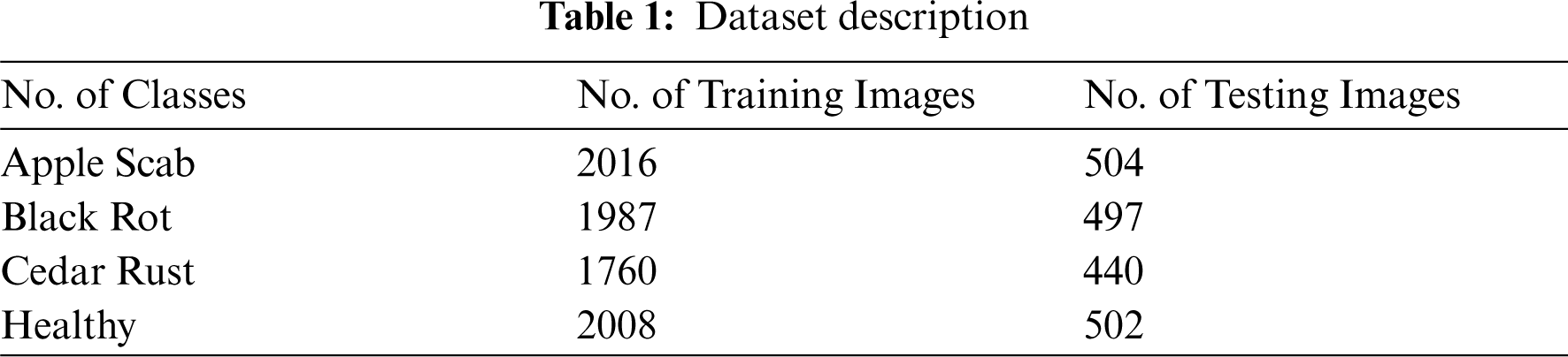
The performance validation of the AIE-ALDC technique takes place utilizing a new plant disease dataset [20]. The dataset comprises images under four different classes like Apple Scab, Black Rot, Cedar Rust, and healthy images. Firstly, the Apple Scab contains a set of 2016 training images and 504 testing images. Besides, the black rot class includes a total of 1987 training images and 497 testing images. Followed by, the Cedar Rust class encompasses a set of 1760 training images and 440 test images. Finally, the healthy class contains a set of 2008 and 502 training and testing images respectively. The details related to the dataset are shown in Tab. 1 and some sample test images are illustrated in Fig. 1.

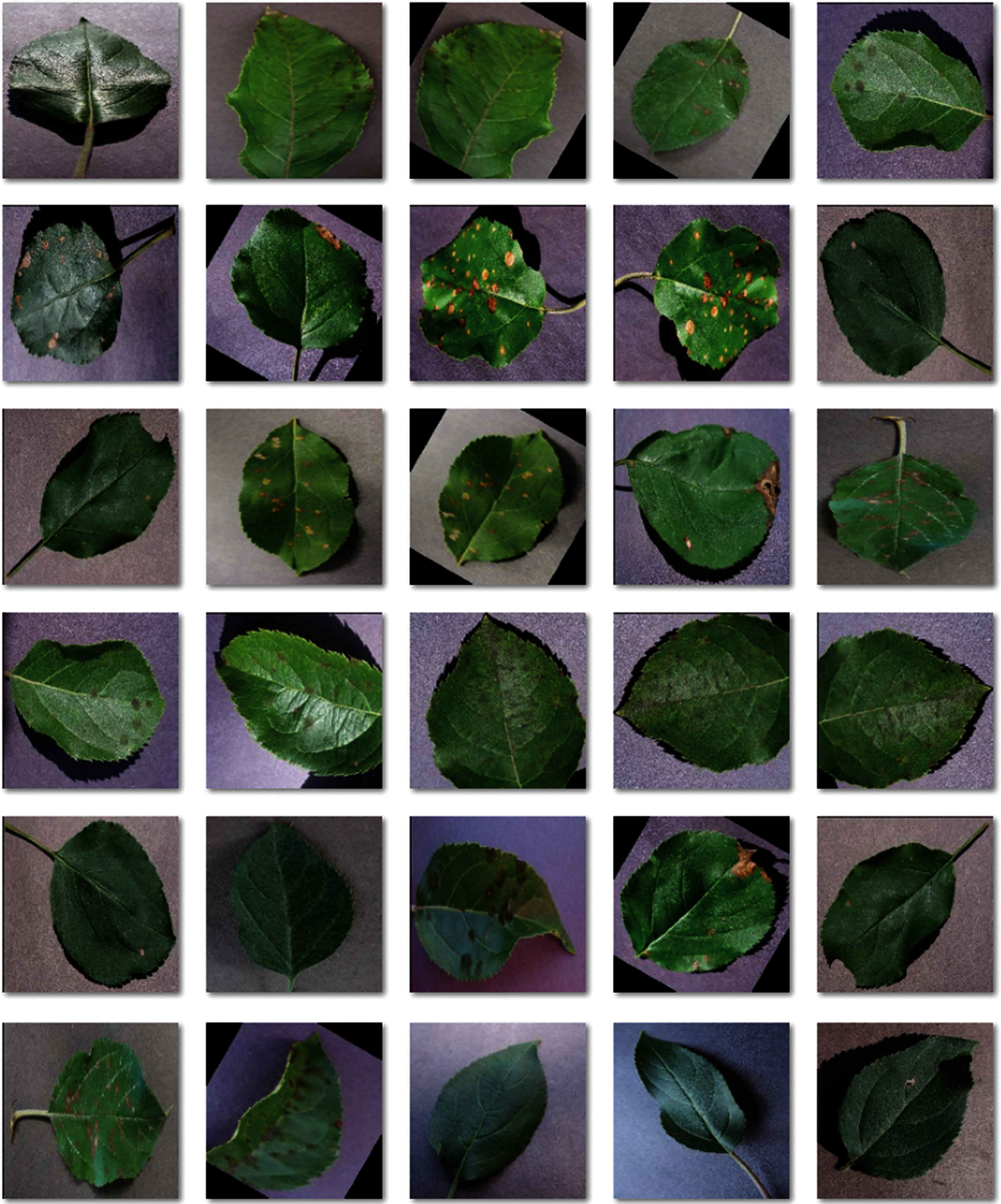
Figure 1: Sample images

3.2 Data Augmentation and Data Pre-Processing

In the apple orchard, the comparative location of the image acquisition devices to study objects is defined by their present spatial relation that is based on the shooting location. Thus, it is complex to picture the apple leave pathological images from all angles to encounter every opportunity. In this subsection, to test and construct the adaptability of the CNN based method, an extended image dataset is developed from the natural images utilizing mirror symmetry and rotation transformation. Image rotation takes place if all the pixels rotate specific angles nearby the centre of an image. Consider that P0(x0, y0) denotes a random point of image; afterward rotating θ° anticlockwise, the point coordinates are P(x, y). The coordinate of the estimation of 2 points is displayed in Eqs. (1) and (2).

{x0=rcosαy0=rsinα(1)

{x=rcos(α−θ)=x0cosθ+y0sinθy=rsin⁡(α−θ)=−x0sin⁡θ+y0cosθ(2)

As displayed, a pathological image is mirrored and rotated for generating 4 pathological images, where the angle of rotation contains 90°, 180°, and 270.

Fig. 2 shows the sample images produced after the data augmentation process. Fig. 2a depicts the original, 2b–2d depicts the images produced after the rotation of 900, 1800, and 2700. The figure depicted that the input images are effectively augmented into different views.

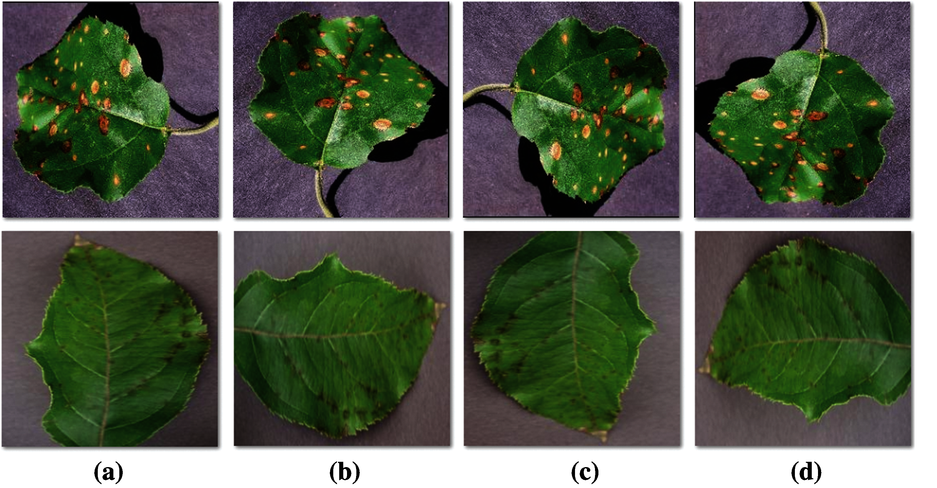
Figure 2: Sample augmented images a) Original image b) 90◦ Rotated image (c) 180◦ Rotated image (d) 270◦ Rotated image

The implementation of two dimensional Gaussian filters was widely utilized for noise removal and smoothing. It requires huge processing resources and the efficacy in executing is stimulating research. The convolutional operator is determined as Gaussian operator and proposal of Gaussian smoothing is attained using the convolution. The Gaussian operator in one dimension is given by:

G1D(x)=12πσe−(x22σ2)(3)

The optimal smoothing filter for the image endures localization in the frequency & spatial domains, in which the ambiguity relations are fulfilled by:

ΔxΔω≥12.(4)

The Gaussian operator in two dimensions is established by:

G2D(x,y)=12πσ2e−(x2+y22σ2)(5)

Whereas, σ (Sigma) denotes the SD of a Gaussian function. Once it has a maximal value, the image smoothing will be higher. (x,y) represents the Cartesian coordinate of the image which showcases the window dimension.

Fig. 3 displays the sample set of pre-processed images produced by the GF technique. From the figure, it is obvious that the quality of the images is considerably enhanced by the GF technique.

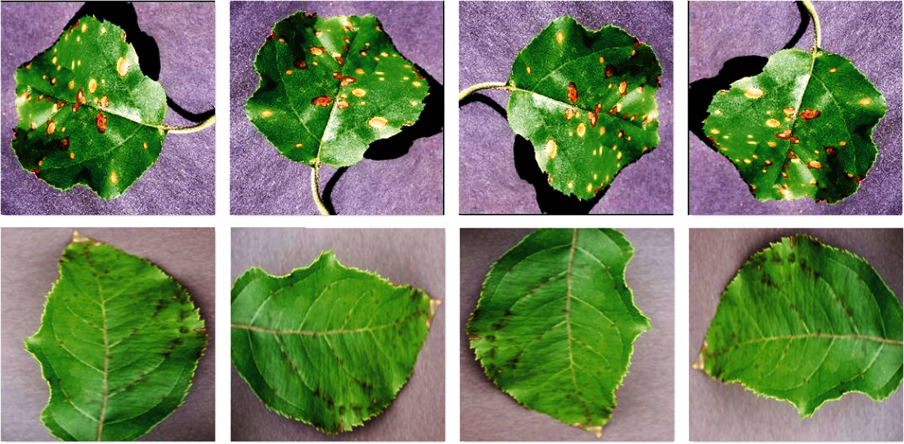
Figure 3: Preprocessed images

3.3 Feature Extraction: WWO-Capsnet Model

Convolutional neural networks (CNNs), or convents for short, is specific kind of FFNN. They are equivalent to the NN demonstrated above in that they are composed of neurons with learnable biases and weights. The significant variation is that the CNN framework creates the implicit statement that the input is an image that permits encoding specific features in the framework. Particularly, convolution captures translation invariance (viz., filter is independent of the position). This alternately creates the forward function more effective, massively decreases the amount of variables, and thus creates the network easier for optimizing and lesser based on the size of the data. A CNN contains MLP, sequence of layers, in which all the layer converts the activation or output of the prior layer by other distinguishable functions. It has many layers utilized in CNN, and this would be described in the following section, but, the most popular components would meet in all the CNN framework contains the fully connected layer, pooling layer, and convolutional layers. Basically, this layer contains, dimensionality reduction, classification layers, and feature extractors, correspondingly. These CNN layers are stacked to create a full convolutional layer. These sliding filters are generally executed by a convolution and, a linear operator, it could be stated as a dot product for effective execution. In every convolution layer, they have a whole set of filters, all of them would generate distinct activation maps. This activation map is stacked for obtaining the output map or activation amount of layers.

The CapsNet method is the most common study field in the research. The fundamental units of CapsNet are capsule that has a group of arranged neurons. The capsule length is based on the invariance, where the amount of features for recreating the image are the measurement of equivariance. Capsule produces vectors of a similar magnitude with distinct locations. The output of capsule i was considered as ui, and conversion matrix Wij was utilized to the capsule output for calculating predictions of parent capsule j by altering ui to the predictive vector U^j|i.

U^j|i=Wijui(6)

whereas U^j|i denotes the predictive vector of output of the jth capsule in a high level calculated by capsule i in layer below, and Wij represents the weighting matrix which should be learned in the backward pass. The variable sj is a weighted amount on the entire predictive vectors uj|i whereas cij denotes the coupling coefficient computed using the dynamic routing procedure for determining conformation degree among the capsules in the layer below and parent capsule [21]. Fig. 4 illustrates the structure of CapsNet.

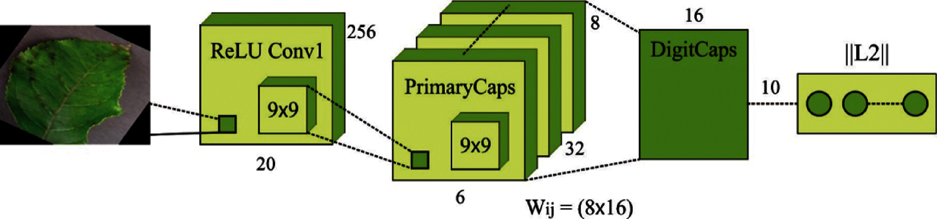
Figure 4: Structure of CapsNet

An activation function baptized squashing shrink the last output vector to 0 when it is smaller and for unit vector when it is larger, for generating capsule length. In activity vectors vj is computed by the succeeding nonlinear squashing functions.

vj=||sj||21+sj||2sj||sj||(7)

The cij is estimated as softmax ofbij. The coupling coefficient is determined as the confirmation degree among the capsule and the parent capsule.

cij=exp(bij)∑kexp(bik)(8)

bij denotes similar score which considered feature and likeliness properties instead of likeliness in neurons.

bij=bij+U^j|ivj(9)

Once the images are augmented and preprocessed, the WWO-CapsNet technique is applied to generate a useful set of feature vectors.

WWO module is an effective and well-known method that has attained greater emphasis from the researchers utilized to map search space problems to a sea bed. Now, a single WW is suggested as a solution where height and wavelength fitness λ. Firstly, h denotes a constant, andλ is assigned as 0.5. It is obvious that a seabed of WW is greater compared to fitness. For optimization procedure, three stages have been executed, Refraction Propagation, and Breaking [22].

3.3.1 Propagation State

For each iteration, all WWs are propagated effectively. With the consideration of actual WWx, the propagated WW and propagation process is a dimension of high functionF, called asD. The propagation process x′ was executed by calculating the operations as Eq. (10)

x′(d)=x(d)+rand(−1,1)⋅λL(d)(10)

whereas d∈D,x(d) denoted the d−th dimension of actual WW x,x(d) indicates the d−th dimension of propagated WW, rand(−1,1) determines an equally distributed arbitrary value amongst −1 and 1, and λ indicates the wavelength of WW, L(d) represents the length of d−th dimensional of search space. Eventually, when the length is greater compared toL(d), then it is arbitrarily set to a new position on the basis of Eq. (11).

L(d)=lb(d)+rand.∗(ub(d)−lb(d))(11)

Whereas lb(d) & ub(d) denotes lower & upper bounds of L(d) and rand. denotes an arbitrary value amongst zero and one. A fitness measure f(x′) is defined by a FF f when finishing propagation process. if h=0,x is substituted, and a wave height is recreated toh\; max\; , otherwise, the actual WW will be preserved and height is shown in Eq. (10) for accelerating the energy dispersion of WW of propagation task [23]. When the iteration is finished, wavelength of a WW is re-calculated by Eq. (12).

λ=λ⋅α−(f(x)−fmin+ε)/(fmax−fmin+ε)(12)

whereas α indicates the wavelength, fmax and f\; min\;  denotes the higher and lower fitness values of current population. ε represents a tiny positive value. It is learned that has maximal fitness value which results in constrained wavelength and tiny range of WW propagation. Now, WW with maximal fitness improves local search.

3.3.2 Breaking State

In the event of WW standard, improved power of WW enhances steeper peak. If speed of wave is greater, WW may be separated into huge amount of solitary waves. With WWO method, the wave breaking task is calculated on newly recognized solution when finishing the propagation operation. A method of separating waves are chosen arbitrarily amongst [1,k\; max\; ],k\; max\;  denotes a predetermined parameter which is higher compared to one, and generates an orphan wave in all dimensions based on Eq. (13).

x′(d)=x(d)+N(0,1)⋅βL(d)(13)

Whereas β represent a coefficient of breaking waves (0.001 and 0.1). N(0,1) indicates a normal distribution. When the wave function is separated, the fitness value of solitary waves is lesser compared tox∗, x∗ is preserved. Succeeded by, x∗ is swapped by an optimal solution of unique waves.

3.3.3 Refraction State

Once WW refracts in the mountain valley, particularly in steep regions with deep sea features. For accelerating the power dispersion of WW in propagation development, henceforth wave height is decreased afterward propagation for removing search stagnation. Eq. (14) is applied for updating the position of a dimension afterward WW refraction:

x′(d)=N(x∗(d)+x(d)2,|x∗(d)−x(d)|2)(14)

Whereas x∗ represents the optimum value of current populations. N(μ,σ) indicates a Gaussian distribution. Succeeded by, a wave height x′ is assigned toh\; max\; , and wavelength of WW is maximalized by Eq. (15).

λ=λf(x)f(x)(15)

3.4 Image Classification

Finally, the BiLSTM model is utilized as a classifier to allot proper class labels to the input apple leaf images. Generally, an RNN is made up of difficulties in learning long term dependency [24]. An LSTM based technique is expanded for RNNs that can able to handle reducing gradient problems. Therefore, the LSTM technique learns the data importance to remove/preserve. Usually, an LSTM technique has output, forget, and input gates. Fig. 5 demonstrates the architecture of LSTM.

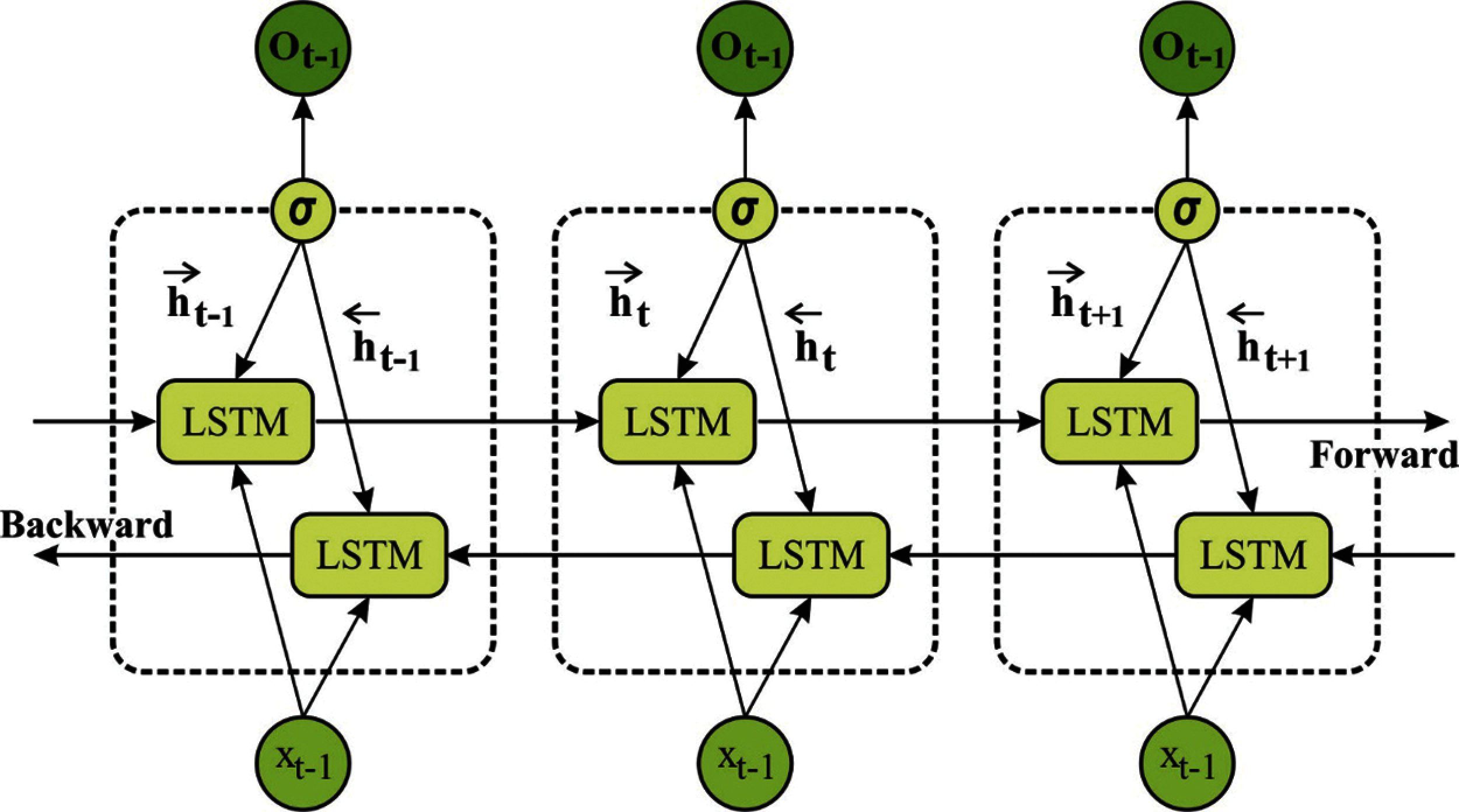
Figure 5: Structure of LSTM

Forget Gate. The sigmoid function is normally employed for creating a decision that should be deleted from the LSTM memory. This decision is basically depending upon the value of ht−1 and xt. A result of this gate is ft, a value among zero & one, while zero represents the learned value, and one denotes the entire value. The result is estimated by:

ft=σ(Wfh[ht−1],Wfx[xt],bf)(16)

whereas bf denotes a constant and so named bias value.

Input Gate. Now, it improves the decision of new data is within the LSTM memory. It can be made up of: sigmoid and “tanh” layers. The results of 2 layers are estimated by:

it=σ(Wih[ht−1],Wix[xt],bi)(17)

ct=tanh(Wch[ht−1],Wcx[xt],bc)(18)

whereas it denotes the value should be upgraded or not, and ct represents a vector of novel candidate value that is added to the LSTM memory. The succeeding formula indicates its numerical formula:

ct=ft∗ct−1+it∗ct(19)

whereas ft denotes the result of forgetting gate that the value amongst zero and one signifies lastly obtained value; however, one represents lastly preserve the value.

Output Gate. It employes sigmoid layer to make decisions i.e., A separation of LSTM memory provides to the result. Next, it creates a nonlinear\; tanh function for mapping the values amongst −1 & 1. The succeeding formula indicates the equations to calculate the result:

ot=σ(Woh[ht−1],Wox[xt],bo)(20)

ht=ot∗tanh(ct)(21)

whereas ot denotes the outcome value, and ht denotes the value amongst −1 & 1.

4  Performance Validation

Fig. 6 displays the confusion matrices generated by the AIE-ALDC technique under different runs. On the execution run-1, the AIE-ALDC technique has classified a set of 484 images into Apple Scab, 489 images into Black Rot, 425 images into Cedar Rust, and 494 images into Healthy. Also, on the execution run-2, the AIE-ALDC approach has classified a set of 494 images into Apple Scab, 489 images into Black Rot, 429 images into Cedar Rust, and 494 images into Healthy. Moreover, on the execution run-3, the AIE-ALDC method has categorized a set of 494 images into Apple Scab, 490 images into Black Rot, 431 images into Cedar Rust, and 494 images into Healthy. Furthermore, on the execution run-4, the AIE-ALDC manner has classified a set of 497 images into Apple Scab, 493 images into Black Rot, 433 images into Cedar Rust, and 498 images into Healthy. Finally, on the execution run-5, the AIE-ALDC methodology has ordered a set of 500 images into Apple Scab, 495 images into Black Rot, 436 images into Cedar Rust, and 500 images into Healthy.

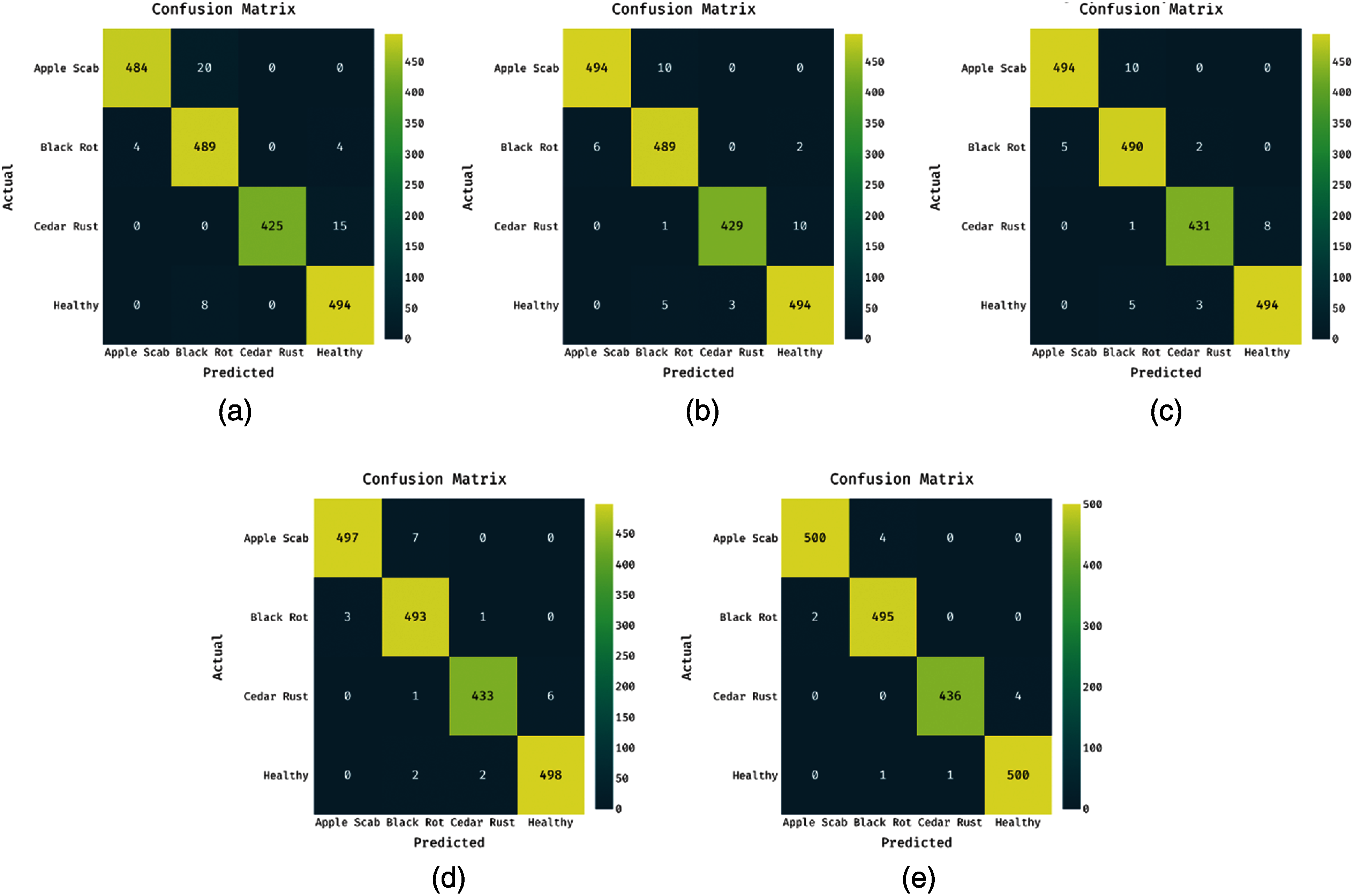
Figure 6: Confusion matrices of AIE-ALDC technique. a) Run-1 b) Run-2 c) Run-3 d) Run-4 e) Run-5

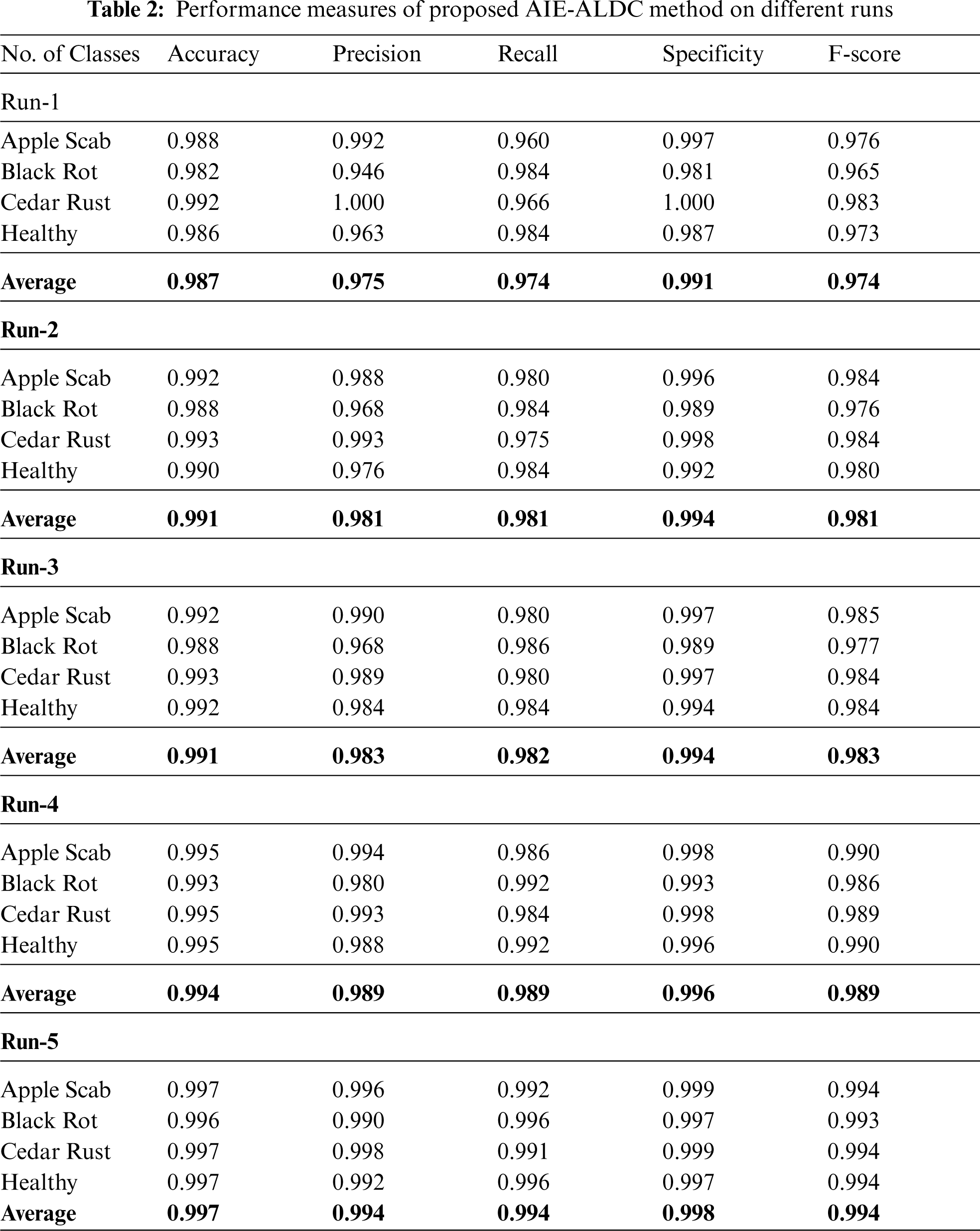
The proposed AIE-ALDC technique is simulated utilizing Python 3.6.5 tool. A deiled classification results analysis of the AIE-ALDC technique is examined under different runs in Tab. 2. From the results, it can be noticed that the AIE-ALDC approach has accomplished maximal apple leaf disease detection performance. For instance, with the execution-1, the AIE-ALDC technique has obtained effectual outcomes with accuracy of 0.987, precision of 0.975, recall of 0.974, specificity of 0.991, and F-score of 0.974. Likewise, with the execution-2, the AIE-ALDC manner has gained effective results with accuracy of 0.991, precision of 0.981, recall of 0.981, specificity of 0.994, and F-score of 0.981. Similarly, with the execution-3, the AIE-ALDC method has attained efficient outcomes with an accuracy of 0.991, precision of 0.983, recall of 0.982, specificity of 0.994, and F-score of 0.983. Also, with execution-4, the AIE-ALDC methodology has gained effectual outcomes with accuracy of 0.994, precision of 0.989, recall of 0.989, specificity of 0.996, and F-score of 0.989. At last, with the execution-5, the AIE-ALDC algorithm has achieved effective results with accuracy of 0.997, precision of 0.994, recall of 0.994, specificity of 0.998, and F-score of 0.994.

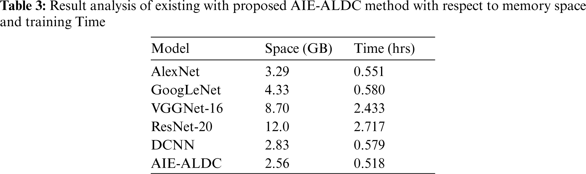
Tab. 3 offers the memory space and training time analysis of the AIE-ALDC technique with other techniques. From the table, it is apparent that the ResNet-20 model has shown ineffective outcomes with a higher memory space of 12 GB and training time of 2.717 h. Followed by, the VGGNet-16 model has gained slightly enhanced performance with a memory space of 8.70 GB and training time of 2.433 h. Then, the GoogleNet and AlexNet models have showcased moderate memory space and training time. At the same time, the DCNN model has portrayed somewhat considerable memory space of 2.83 GB and training time of 0.579 h. However, the AIE-ALDC technique has outperformed the other techniques with a minimal memory space of 3.29 GB and training time of 0.551 h.

In order to ensure the promising performance of the AIE-ALDC technique, a detailed comparison study is made with the recent methods in Tab. 4 and Fig. 7 [25]. From the obtained values, it is noticeable that the BP and SVM models have led to least outcome with the accuracy of 0.5463 and 0.6873. In line with, the ResNet-101 and AlexNet models have depicted slightly enhanced outcome with the accuracy of 0.9116 and 0.9119. Then, the ResNet-50, ResNet-20, ResNet-34, and ResNet-18 models have demonstrated moderate outcome with the accuracy of 0.9317, 0.9364, 0.9549, and 0.9569 respectively. Followed by, the VGGNet-16 model has gained somewhat considerable outcome by gaining an accuracy of 0.9632. Though the DL-ICNN and DCNN models have portrayed competitive accuracy values of 0.9714 and 0.9762, the proposed AIE-ALDC technique has surpassed all the other techniques by accomplishing a maximum accuracy of 0.992.

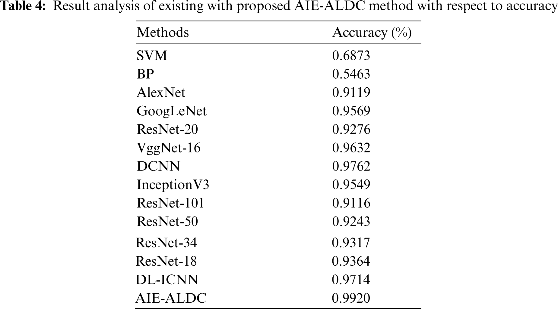
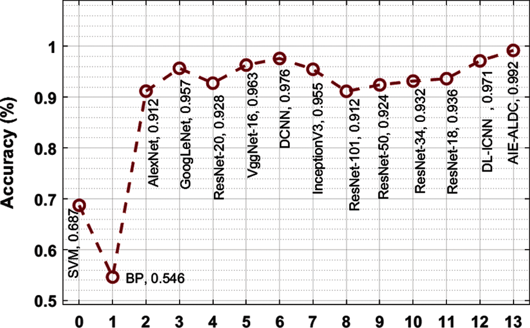
Figure 7: Accuracy analysis of AIE-ALDC model with existing techniques

By looking into the aforementioned tables and figures, it can be ensured that the AIE-ALDC methodology is initiate that exists an appropriate technique for apple leaf disease detection and classification.

5  Conclusion

This paper has devised an efficient AIE-ALDC technique for the detection and classification of apple leaf diseases. The proposed AIE-ALDC technique encompasses orientation based augmentation, GF based preprocessing, CapsNet based feature extraction, WWO based parameter tuning, and BiLSTM based classification. The use of WWO algorithm aids to optimally adjust the hyperparameter involved in the BiLSTM model. A wide range of experiments was performed to showcase the supremacy of the AIE-ALDC approach. The experimental outcomes demonstrate the promising performance of the AIE-ALDC technique over the recent state of art methods with the higher accuracy of 0.9920. In future, the proposed AIE-ALDC technique can be deployed in a real time environment using internet of things (IoT) and imaging sensors.

Funding Statement: The authors extend their appreciation to the Deanship of Scientific Research at King Khalid University for funding this work under Grant Number (RGP2/209/42), https://www.kku.edu.sa. This research was funded by the Deanship of Scientific Research at Princess Nourah bint Abdulrahman University through the Fast-Track Path of Research Funding Program.

Conflicts of Interest: The authors declare that they have no conflicts of interest to report regarding the present study.

This work is licensed under a Creative Commons Attribution 4.0 International License, which permits unrestricted use, distribution, and reproduction in any medium, provided the original work is properly cited.