Computers, Materials & Continua DOI:10.32604/cmc.2022.021716
Article

Deep Learning Based Intelligent Industrial Fault Diagnosis Model

R. Surendran1,*, Osamah Ibrahim Khalaf2 and Carlos Andres Tavera Romero3

1Center for Artificial Intelligence & Research (CAIR), Chennai Institute of Technology, Chennai, 600069, India
2Al-Nahrain Nanorenewable Energy Research Center, Al-Nahrain University, Baghdad, 64074, Iraq
3COMBA I+D Research Group of Universidad Santiago de Cali, Santiago de Cali, Colombia
*Corresponding Author: R. Surendran. Email: dr.surendran.cse@gmail.com
Received: 12 July 2021; Accepted: 18 August 2021

Abstract: In the present industrial revolution era, the industrial mechanical system becomes incessantly highly intelligent and composite. So, it is necessary to develop data-driven and monitoring approaches for achieving quick, trustable, and high-quality analysis in an automated way. Fault diagnosis is an essential process to verify the safety and reliability operations of rotating machinery. The advent of deep learning (DL) methods employed to diagnose faults in rotating machinery by extracting a set of feature vectors from the vibration signals. This paper presents an Intelligent Industrial Fault Diagnosis using Sailfish Optimized Inception with Residual Network (IIFD-SOIR) Model. The proposed model operates on three major processes namely signal representation, feature extraction, and classification. The proposed model uses a Continuous Wavelet Transform (CWT) is for preprocessed representation of the original vibration signal. In addition, Inception with ResNet v2 based feature extraction model is applied to generate high-level features. Besides, the parameter tuning of Inception with the ResNet v2 model is carried out using a sailfish optimizer. Finally, a multilayer perceptron (MLP) is applied as a classification technique to diagnose the faults proficiently. Extensive experimentation takes place to ensure the outcome of the presented model on the gearbox dataset and a motor bearing dataset. The experimental outcome indicated that the IIFD-SOIR model has reached a higher average accuracy of 99.6% and 99.64% on the applied gearbox dataset and bearing dataset. The simulation outcome ensured that the proposed model has attained maximum performance over the compared methods.

Keywords: Intelligent models; fault diagnosis; industrial control; deep learning; feature extraction

1  Introduction

In recent times, the operational status observance and fault analysis of rotating machinery is highly significant. Rotating machineries are becoming essential equipment in the industrial sector [1]. In the last decades, the robust deployment of effective rotating machinery like the latest supersonic vector aircraft engine, massive generator set, accurate machine tool spindle, and efficient marine propulsion motor, and many other devices are developed for achieving automation, unmanned operations, and maximum speed. To approve their security and scalability, it is mandatory to develop proficient and smart fault diagnosis and health monitoring models. Generally, vital faults progress from incipient micro faults gradually. Incipient faults provide minimal consequence on the reliability of the rotating machinery , and are highly simple and easily managed. Therefore, the characteristics of incipient faults are not so reliable, while predicting the micro-faults is complex when compared with normal faults. In recent times, incipient micro-fault analysis and observation models are examined extensively in fault diagnosis. Fault diagnosis approaches are classified into two classes namely, a mechanism analytical model as well as data-driven models. The major requirement is to develop a higher precision numerical approach for defining the establishment of fault diagnosis. Even though better results can be obtained, it is not possible to achieve higher precision in such a model. Additionally, the newly developed method is highly tedious to transplant and resolve related issues [2]. Hence, in the enhancing complexities of mechanical systems, fault diagnosis models have relied on mechanical analytical methods that are applied to a certain extent.

In recent times, an extensive application of the Internet of Things (IoT), advanced intelligent sensing devices, and data collection methodologies are applied vastly in rotating machinery automation. Most of the monitor data like vibrations, sound, temperature, power, and pressure of rotating machinery can be attained effortlessly, and the previous data saves the health details of rotating machinery from starting to the termination of the service. Hence, engineers compute fault diagnosis using statistical analysis of massive historical information. Currently, the data-driven fault diagnosis technique is well-known and used in several applications [3]. For instance, the Yangtze Three Gorges Hydropower Station of China is composed of huge hydroelectric generator sets. Every generator set has to observe various status indications like vibrations, artifacts, pressure enhancement, and so on. The data observation of every indicator is represented by Terabytes (TB). Thus, it becomes impossible to know the experience of engineers for examining the faults while computing feature extraction manually. It is highly prominent in maximum applications like aircraft engines, smart ships, unattended vehicles, and independent ships. Therefore, it is significant to develop intelligent, automated, and adaptive data-driven fault analysis models. Recently, with the considerable development of Machine Learning (ML) and Deep Learning (DL) methodologies, fault diagnosis approaches rely on them is now being current research.

Contrasting from conventional fault diagnosis models relied on the signal processing method; intelligent diagnosing schemes are used for extracting applicable features from monitoring data in the industrial sector. The general intelligent diagnosis models have 3 phases namely, feature extraction, feature selection (FS), and fault classification. Initially, feature extraction transforms the actual data signals gathered by numerous sensors in both the time and frequency domain to reliable representative features for fault identification. Secondly, FS eliminates lower sensitivity and unwanted data from collected features. Thirdly, fault identification feeds the collected features to the fault classifier and compute pattern analysis and, lastly, results in classification results by frequent iterative training. By the utilization and validation, the predefined approaches have inferior feature extraction potential because of the shallow network architecture, and it is not easy to apply in the alternate application, especially for big data [4]. Presently, developers have unified manual feature extraction and shallow ML methodologies for computing intelligent fault diagnosis [5]. In recent times, DL and Deep Neural Networks (DNN) models have gained maximum attention among researchers and are used in mechanical fault diagnosing operations.

This paper develops an Intelligent Industrial Fault Diagnosis using Sailfish Optimized Inception with Residual Network (IIFD-SOIR) Model. The proposed model involves three processes such as signal representation, feature extraction, and classification. Initially, the Continuous Wavelet Transform (CWT) is applied to achieve a pre-processed representation of raw vibration signals. Afterward, Inception with ResNet v2 (IRV2) based feature extraction model is employed to create a set of high-level features. It is chosen over the other DL models because it possesses a shortcut connection at the left of each module. In addition, it has roughly the computational cost of Inception-v4. Additionally, the training of the IRV2 model is faster and got slightly better final accuracy than Inception-v4. Also, the way of fixing the hyperparameters of the IRV2 model necessitates knowledge and widespread trial and error. As there are no simpler and easy methods available for fixing the hyperparameters of the IRV2, the proposed model makes use of a sailfish optimizer (SFO) to tune them. Lastly, a multilayer perceptron (MLP) is applied as a classification tool to identify the faults capably. The utilization of SFO for the hyperparameter tuning of IRV2 in the fault diagnosis process shows the novelty of the work. Extensive experimentation takes place to ensure the effective outcome of the IIFD-SOIR method on the gearbox dataset and a motor bearing dataset.

The organization of the paper is given as follows. Section 2 briefs the related works, Section 3 proposes the IIFD-SOIR model, Section 4 simulates the presented model, and finally, Section 5 concludes the paper.

2  Literature Review

Awan et al. [6] projected a 5-layer DNN approach such as 3 hidden layers under the application of a deep autoencoder scheme to identify faults in rolling bearing and planetary gearbox; however, the actual data required is converted to the frequency spectrum. Khan et al. [7] applied a DNN framework based on Deep Belief Network (DBN) applied to diagnose faults in aircraft engines and a power transformer. Li et al. [8] employed a 3 layer DNN that relied on DBN to identify faults in rolling bearing and devices. But, in this approach, the faults are accelerated by grooving, and the fault characteristics are considered as an essential fault, that shows the efficiency and capability of the method while resolving the problems of micro-fault diagnosis. Convolutional Neural Network (CNN) was coined by Prasad et al. [9]. It is highly significant in the DL application [10]. When compared with DNN, the CNN approach consists of a minimum number of parameters because of shared filters [11].

CNN is significantly capable of extracting effective features and is mainly employed in image analysis [12]. Recently, developers have used CNN for the application of identifying faults. Xia et al. [13] projected a DNN technique by stacked CNN for diagnosing faults in rolling bearing and gearbox. Thus, it still requires additional frequency spectra of actual data. Abdulsaheb et al. [14] employed a DL model under the application of the CNN technique for fault diagnosis of rolling element bearings. Though the predefined methods are applied in the CNN model, it still requires a classical traditional feature extraction technology for extracting useful features from original vibration data. Additionally, this model has not applied the entire efficiency of CNN in extracting features that have a minimum enhancement in diagnosing faults. Zhang et al. [15] applied a 2-D representation of actual vibration signals input for a CNN approach and compute the fault diagnosis of bearings. Even though these models are lagging in manual feature extraction from actual data, a major limitation is present in this scheme. In the CNN model, the Fully Connected (FC) network has been employed. The parameter quantity of FC structure in the CNN model is maximum and results in massive time consumption for training and testing. These constraints have an undesirable effect on quick fault identification as well as real-time prediction of micro-faults.

3. The Proposed IIFD-SOIR Model

Fig. 1 shows the process involved in the IIFD-SOIR model. As depicted in the figure, the data acquisition process takes place to collect the data. Then, the Continuous Wavelet Transform Scalogram (CWTS) model is applied to preprocess and crop the vibration signals. Followed by, the SFO algorithm tuned Inception with ResNetv2 model is implemented as a feature extractor. Finally, MLP is applied as a classification model to identify the different kinds of faults.

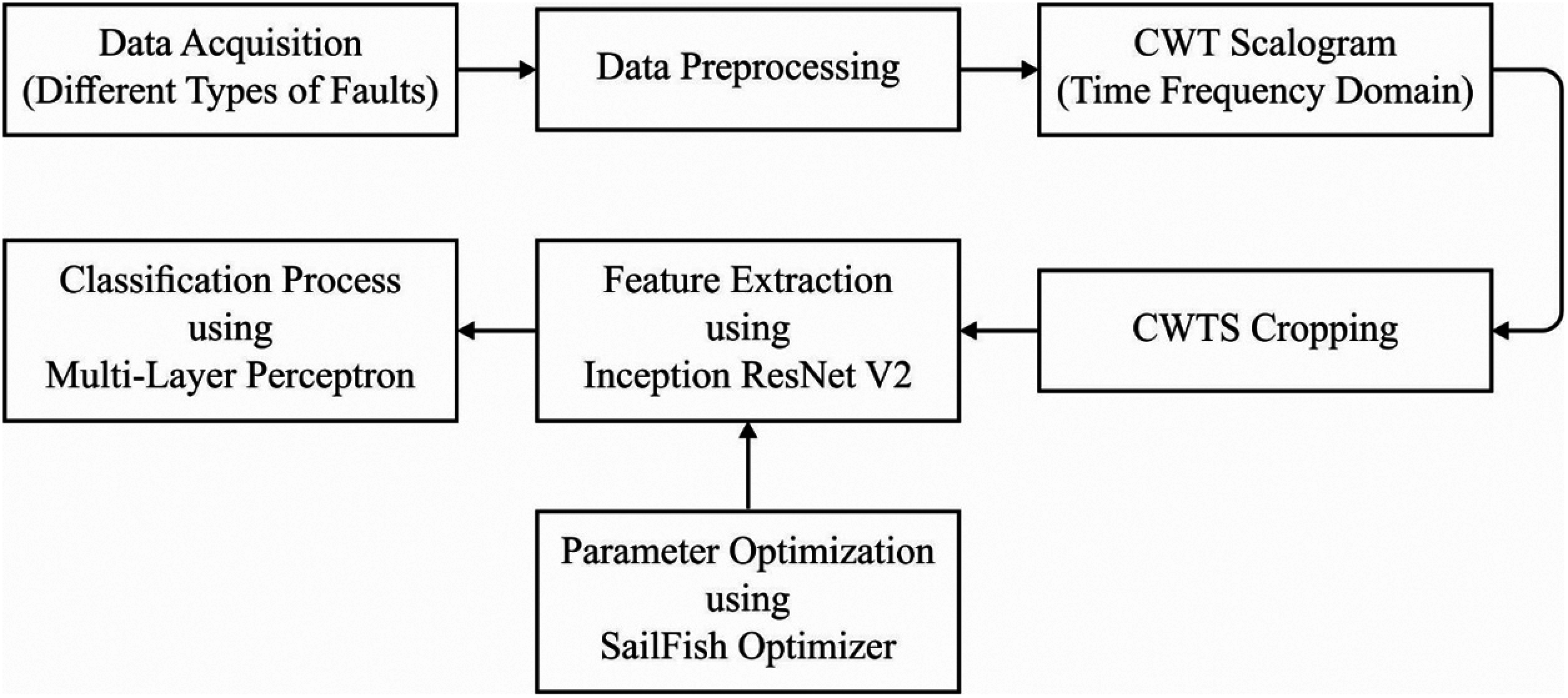
Figure 1: Block diagram of IIFD-SOIR model

3.1 Data Collection and Preprocessing

Rotating machinery is a function of different rotating speeds and loads. For performing fault identification in several functioning states, the vibration signal from the machine in the total speed and load range required for obtaining to train it [16]. But, when the instance frequency of the signals is dissimilar to the rotating frequencies, several rotating speeds are the reason for an extensive variation in CWTS. For eliminating these controls, the vibration signal is gathered with the rotating speed data. Noticeably, the rotating speed in the training sample is regarded as constant as it can be gathered if the machinery is in a constant functioning form. Initially, the DC module of the vibration signal is eliminated as it does not provide error analysis. A DC part is eliminated by performing subtraction of the mean value of the signal. As the rotating speed modifies in function if the functioning mode modifies, load modifies, and in start-up and shutdowns, the CWTS gives essentially several outcomes when the signals at rotating speed are not preprocessed. For eliminating the control of rotating speed on CWTS, signal re-sampling with a virtual re-sampling frequency (VSF) is established. For vibration signal in the training samples, since its rotating speed is identified, VSF is a group as a frequency namely q multiples of the rotating speed. Noticeably, q stays similar to every training sample. By this re-sampled vibration signal, all rotations of the rotor have the Assume the vibration signal x(k)(k=1,2,…,m), it is gathered at a sampling frequency f(Hz) with m sample datapoints. Rotating speed is n (rpm), equivalent to a machine rotating frequency fm=n/60. Determine fd as the virtual re-sampling frequency which is the needed several times of the fm i.e., fd=qfm, in which q is the needed several numbers. For unifying the sampling frequency as fd, the data is processed as follows.

By resampling frequency fd, the k-th resampled data point must be x¯(k)=x(kffd). When f is a multiple of fd, after that, it only requires selecting x(i×ffd),(i=1,2,3,⋯) as the novel x¯(k). If not, utilizing a quartic polynomial interpolation operation Φ through the actual instances about x(⌊kffd⌋), the novel x¯(k)(k=1,2,3…,) is attained by utilizing Eq. (1):

K →=(⌊kffd⌋−1, ⌊kffd⌋,⌊kffd⌋+1, ⌊kffd⌋+2)(1)

Every data has a comparable length behind pre-processing at sampling frequencies that are similar multiples of the rotational frequencies. The wavelet transform decays a signal in the time-frequency field by utilizing relatives of wavelet functions. Scaling and translation of an essential wavelet function are defined by:

Ψa,b(t)=|a|−12Ψ(t−ba)a, b∈Ra≠0 (2)

where Ψa,b(t) is a continuous wavelet, ais the scalable variable, and b, the translational variable, correspondingly.

CWT take over and made the localization design of the short-time Fourier transform (STFT). A CWT is used for signal time-frequency diagnosis and processing. A CWT of a signal x(t) is determined as the convolution of the signal x(t) with the wavelet function Ψa,b(t). During this technique, the CWT is performed for decomposing the information from scale 1 to l, in which l is generally equivalent or superior to, 2q:

Ca(k)=∫⁡x(t)⋅Ψ¯a,b(t)dt(3)

in which Ca(a=1,2,3, …, l) is the wavelet coefficient of x(t) at the a th scale and Ψ¯a,b(t) is the difficult conjugate of the wavelet operation at scaling a and translation b The CWT creates the coefficients on the several parts of the signal in several scaling factors. Utilizing this wavelet coefficient, a signal in the time-frequency field is straightly illustrated by a 2-D image. A graph of the wavelet coefficients generates the CWTS.

Getting every wavelet coefficient in a matrix P=[C1, C2, …, Cl], it is changed to a gray matrix Pnew by:

Pnew(i,j)=[P(i,j)−pminpmax−pmin×255+12](4)

where pmin and pmax are the minimum and maximum elements of P, correspondingly. A value of the element in Pnew refers to a gray value in the series from 0 to 255. So, Pnew is the CWTS of the original signal.

Massive image recognition necessitates a more complicated CNN architecture and more calculations, which takes longer to train and calculate. Conversely, a massive image is reducing the result of tiny local features and decrease the sensitivity and accuracy of fault analysis. For accommodating this, CWTS cropping is performed using 3 rules:

•   A cropping effect should include at worst the CWT coefficients of 1 whole rotating duration.

•   The length of the one side of the square outcome should be superior to 2q.

When the pixel's coordinate points are greater than the coordinate points on the time axis, the pixel cannot be used as a result. 2.2. Inception with ResNetv2 Model

CNN is a variation of multilayer FC feedforward neural networks (FFNN) that can remove local features to classify data in an automated way. It is extremely utilized in varied computer vision functions. While several variations of the CNN method are made, a structure of the usual CNN is created with a convolution layer, pooling or sub-sampling layer, and FC layer as in a typical multiple NN.

The convolution layer is the important building block of CNN. It can be generally developed for a group of learnable kernels and one trainable bias for every feature map. In the convolutional layer, all filters are linked to the local patches in the feature map of the preceding layer [17]. For input xl-l 1 of the (l−1)th layer, the next layer's feature map is illustrated as follows:

xil=f(∑i=1N⁡xil−1∗kijl+bjl)(5)

where N is the kernel count in (l−1)rh layer; xlj is the jth feature map in the lth layer; k and b are the equivalent convolutional kernel and additive bias, and f(⋅) illustrates the non-linear activation function.

Behind the convolution layer, it is necessary of adding a pooling layer among the CNN layers. It joins the outcome of the neighboring neurons at 1 layer to an individual neuron in the subsequent layer. Individual groups amongst several feature maps are optimal for obtaining further abstract feature illustrations. It can be used for shorting the calculations and manage overfitting by decreasing the dimensionality of the input for reducing the count of parameters. When an input map is available, after that resultant map with diminished size would be attained using a pooling function that is illustrated as:

xjl=f(βjldown(xjl−1)+bjl)(6)

where down(⋅) signifies a sub-sampling or pooling operation, β is the multiplicative bias and b is the additive bias to all feature maps. A final result generally is the softmax that is utilized for classifying the input data into many class labels. Afterward, the training model to CNN is similar to which the usual NN by backpropagation and gradient descent technique.

Inception-ResNet-V2 (IRV2) was developed by Google Company in 2018 which is applied in place of existing approaches for the fault diagnosis of machinery. It is defined as the integration of GoogLeNet and ResNet. This method is composed of 10 portions, where each portion has its responsibility in role orientation as well as function. Here, Inception is a common network with parallel layer infrastructure used in GoogleNet. The filters have parallel connections with various sizes of 1x1, 3x3, and 5x5. The tiny size leads to a convolutional kernel and extracts the image features effectively and limits the model variables. When compared with other sizes, the large-scale convolution kernel would maximize the variables of the model matrix, hence various small-scaled convolution kernels are interchanged in a parallel fashion for eliminating the functional variables. Consequently, the method is applied extensively and more reliable when compared with the former network with Inception. Inception v1–v4 is the general approach of GoogleNet. Thus, the residual learning enabled ResNet is an extension of ILSVRC 2015 that applies 152 layers. ResNet's core assumption is to incorporate a direct link to this method, which is referred to as Highway Network informally. The traditional network structure is defined as a non-linear conversion of functional input, whereas Highway Network enables a limited ratio of a result in the existing network layer. As a result, the actual input data is forwarded directly to the upcoming layer. At the same time, ResNet secures the data by direct transmission of input to output. The entire network has to know the variations among input and output that signifies the learning objectives as well as complexities. ResNet-50, ResNet-101, and ResNet-152 are few modules in ResNet. In Residual-Inception system (Fig. 2), the the Inception block has been applied as it has minimum processing complexity when compared with the actual Inception module. Figs. 2a‒2c implies the Inception ResNet layers, such as Inception ResNet A, Inception ResNet B, and Inception ResNet C. The count of layers is 5, 10, and 5, correspondingly. Figs. 2d and 2e illustrate the Reduction Layer of IRV2, in which Reduction A and Reduction B. Every Inception block is linked to a filter layer for dimension transformation and accomplishes the input mapping. It compensates for the dimensionality reduction in the Inception block. Based on the traditional studies [18], IRV2 evolved from Inception ResNet V1 (IRV1) matches the actual cost of the Inception-v4 network. Regarding this, a small variation among residual and non-residual Inception, especially in Inception-ResNet, is batch normalization (BN) applied in traditional layers. Because tests have shown that using the maximal activation size requires a lot of GPU RAM, large Inception modules may be made by removing the BN layer once the activation is finished. Also, a method becomes highly effective and précised. Furthermore, when the filter count is above 1000, then the residual network becomes unstable, and premature death will exist in the network training process. Followed by, a huge number of training data is applied, and layer present before the average pooling generates zeroes. It cannot be removed by minimizing the learning rate as well as including BN layers.

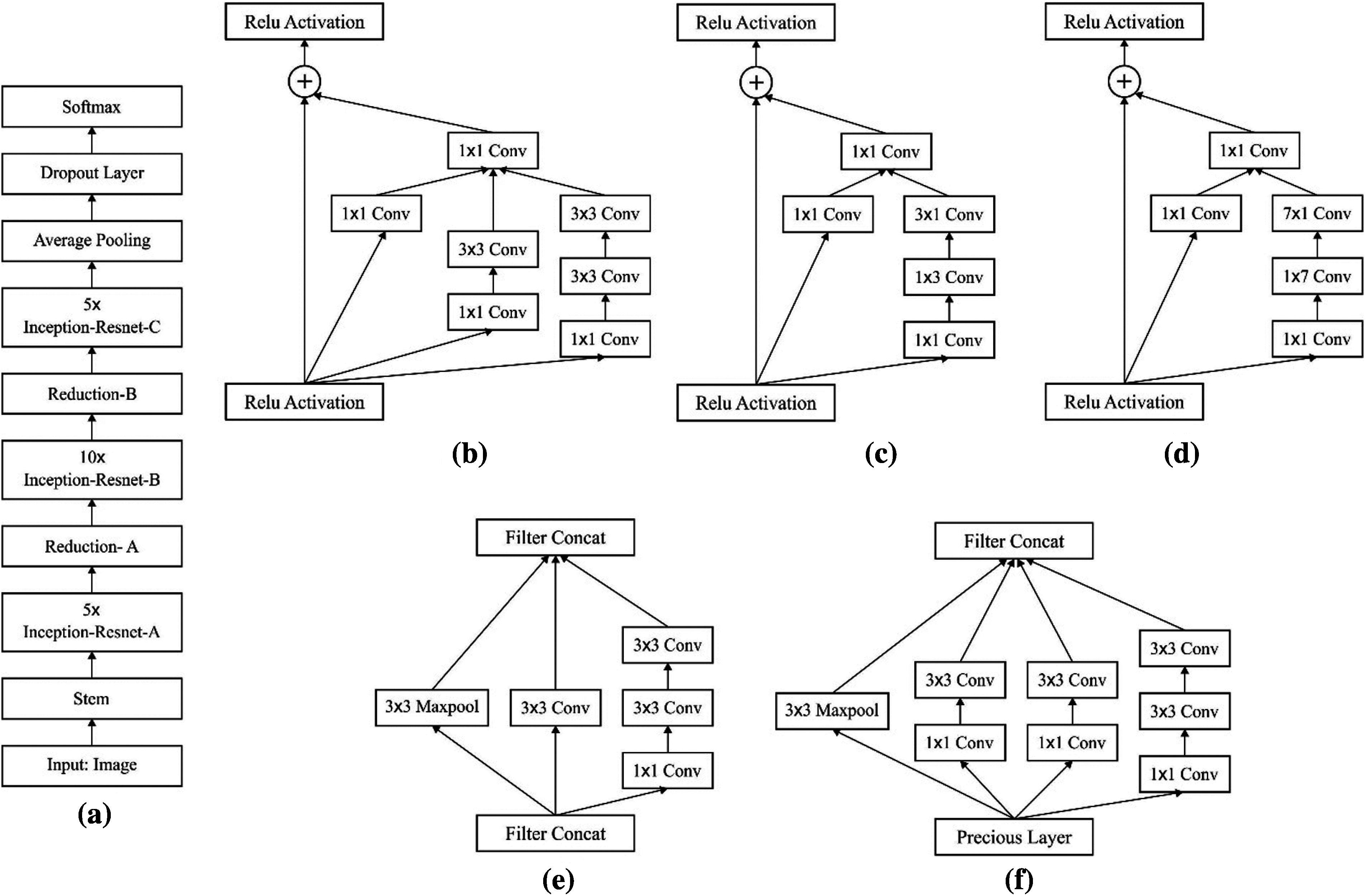
Figure 2: (a) Architecture of inception ResNet V2 (b) Inception ResNet A, (c) Inception ResNet B, (d) Inception ResNet C, (e) Reduction-A, and (f) Reduction-B

3.3 Sailfish Optimizer Based Parameter Optimization

In the Inception with the ResNet v2 model, few main hyperparameters exist namely kernel size, filter count, hidden node count, and penalty coefficient, which majorly influence the overall results. Practically, it is time-consuming and hard to select the proper combination of parameters. To choose the optimal parameters of Inception with the ResNet v2 model, the SFO algorithm is employed. In general, SFO [19] is defined as a population relied meta-heuristic approach that is based on the attack-alternation principle of a group of hunting sailfishes. Sailfishes are assumed to be distributed in the search space, while the place of sardines assists in finding d optimal solution in search space. It has an optimal fitness measure is named as ‘elite’ sailfish and the place at ith iteration is provided by PSlfBesti. For sardine, the affected is a one which has better fitness value and the location at ith iteration is provided by PSrdInjuredi. For all iterations, the place of sardines and sailfishes is maximized. For i+1th iteration, a novel position PSlfi+1 of a sailfish is upgraded by applying ‘elite’ sailfish and ‘affected sardine as given in Eq. (7).

PSlfi+1=PSlfBesti−μi×(rnd×PSlfBesti+PSrdInjuredi2−PSlfi)(7)

where PSlfi implies the former place of Slfth sailfish, rnd defined as an arbitrary value among 0-1 and μi refers to a coefficient produced as per Eq. (8).

μi=2×rnd×PrD−PrD(8)

where PrD describes prey density, which represents the count of prey for all iterations. Followed by, the measure of PrD, is valued by Eq. (9), reduces as the number of preys is limited while group hunting.

PrD=1−NumSlfNumSlf+NumSrd(9)

where NumSlf and NumSrd refers to the value of sailfishes and sardines correspondingly.

NumSlf=NumSrd×Prcnt(10)

where Prcnt defines the ratio of sardine population which develops an initial sailfish population. The primary number of sardines is assumed as superior to the number of sailfishes. The sardine places get upgraded in all iterations as provided by Eq. (11).

PSrdi+1=rnd(0, 1)×(PSLfBesti−PSrdi+ATK)(11)

ATK=A×(1−(2×itr×κ))(12)

where PSrdi and PSrdi+1 represents the former and current locations of sardine correspondingly and ATK implies the sailfish's attacking efficiency at iteration itr. Then, the count of sardines which upgrades the place and number of displacements are based on ATK. The minimization of ATK helps the convergence of the search agent. Under the application of variable ATK, the number of sardines which upgrades the location (γ) and count of variables of them (δ) are determined in Eqs. (13)–(14):

γ=NumSrd×ATK(13)

δ=v×ATK(14)

where v denotes the value of variables and NumSrd implies the count of sardines. When the sardines are facilitated as a fitter compared to any sailfish, the sailfish maximizes the place, as well as the sardine, is removed from its population. Random selection of sailfishes and sardines ensures the identification of the search area. Since the attacking ability of sailfish reduces for all iterations and it offers a chance of escaping from a sailfish, that helps in exploitation. The ATK variable manages to identify a tradeoff among exploration and exploitation. Fig. 3 depicts the workflow of the SFO algorithm.

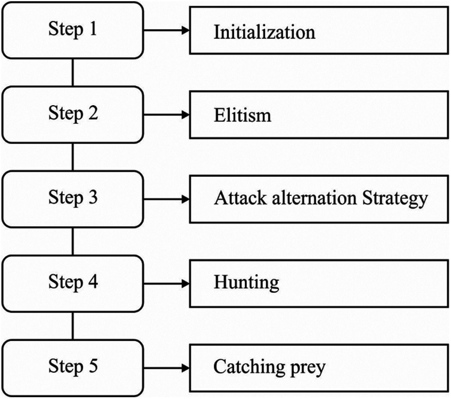
Figure 3: Flowchart of SFO algorithm

3.4 MLP Based Classification

MLP is defined as a NN method with several hidden layers, and neurons among adjacent layers are linked together. The structural representation of this method is depicted in Fig. 4.

The parameter selection is composed of newly presented MLP depends upon the experience and experiment. The hidden layer selection is computed by comparing the experiment by fixing 2, 4, 6, and 8 hidden layers and the attained results demonstrate the layer with enhanced time cost whereas the accuracy is not maximized. If the layer is fixed as 2, the classification accuracy is reduced. Hence, the accuracy and time cost can be balanced by 4 hidden layers applied in this approach. The count of neurons present in a hidden layer is fixed based on multiple trial performance, and the principle is balanced with time cost and accuracy. The activation functions, as well as loss functions, are ReLU and softmax cross-entropy along with logits is employed, correspondingly. The flow of extraction is composed of 3 phases namely, sample selection, model training, and classification generation.

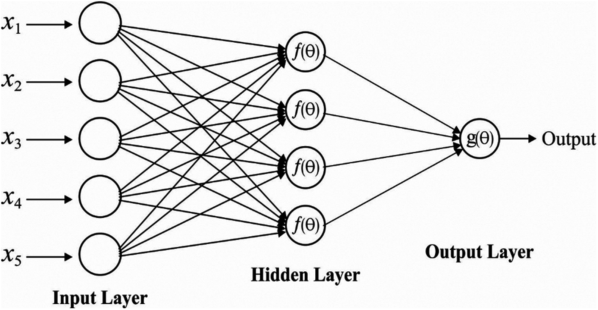
Figure 4: Structure of MLP

4  Performance Validation

4.1 Implementation Data

The performance of the proposed model is simulated using the Python tool. To ensure the effective outcome of the presented model in the identification of various fault class labels, two datasets namely automotive gearbox and bearing fault from Case Western Reserve University Bearing Data Center [20]. The first dataset holds 7 types of health status like an outer race bearing fault, a minor chipped gear fault, a missed tooth gear fault, and three types of compound faults (Normal, Minor chipped tooth, Missing tooth (0.2 mm), and Missing tooth (2 mm)). Under every class label, 1200000 samples are gathered and divided into 100 instances with 0.5 s. Besides, a set of 300 sample instances are attained under every health status with varying speed rates. At last, a dataset with 2100 sample instances is attained. The second dataset has both normal and fault data. The types of bearing fault have Inner race (IF), Outer race (OF), and Ball faults (BF). Therefore, there are atotally of 10 kinds of bearing health status under varying loads. Every sample has a set of 2000 data points, which are again transformed into a time-frequency representation utilizing WT [21,22]. Every health status comprises 60 instances under every load. There are 2400 sample instances gathered to verify the algorithm's performance.

4.2 Results Analysis

Fig. 5 investigates the accuracy analysis of the different fault classes by the IIFD-SOIR model on the applied Gearbox dataset. On the applied gearbox dataset 1, the IIFD-SOIR, FFT-SVM, CNN, and CNN2 models have reached a maximum accuracy of 100%, 100%, 100%, and 100% whereas the FFT-KNN, FFT-DBN, and FFT-SAE models have demonstrated slightly lower performance with the accuracy of 85.44%, 98.90%, 99.97% respectively. Likewise, on the given gearbox dataset 2, the IIFD-SOIR, FFT-SVM, CNN, and CNN2 methodologies have attained a higher accuracy of 100%, 100%, 100%, and 100% while the FFT-KNN, FFT-DBN, and FFT-SAE methodologies have depicted minimal function with the accuracy of 93.46%, 98.87%, 99.98% correspondingly. Likewise, on the applied gearbox dataset 3, the FFT-SVM, FFT-KNN, FFT-SAE, and FFT-DBN approaches have accomplished higher accuracy of 99.89%, 99.71%, 99.64%, and 99.50% whereas the IIFD-SOIR, CNN, and CNN2 methods have illustrated moderate performance with the accuracy of 99.34%, 98.58%, 98% respectively. Meanwhile, on the applied gearbox dataset 4, the FFT-SVM, FFT-KNN, FFT-SAE, and CNN frameworks have achieved a maximum accuracy of 100%, 100%, 100%, and 100% while the IIFD-SOIR, CNN2, and FFT-DBN technologies have depicted considerable function with the accuracy of 99.85%, 99.77%, 99.49% respectively. Then, on the applied gearbox dataset 5, the IIFD-SOIR, FFT-SAE, CNN, and CNN2 schemes have gained optimal accuracy of 100%, 99.98%, 100%, and 100% whereas the FFT-KNN, FFT-DBN, and FFT-SVM approaches have depicted moderate function with the accuracy of 88.07%, 99.41%, 99.90% correspondingly. Moreover, on the applied gearbox dataset 6, the IIFD-SOIR, FFT-SAE, CNN, and CNN2 technologies have attained higher accuracy of 99.26%, 98.24%, 99.76%, and 97.74% while the FFT-KNN, FFT-DBN, and FFT-SVM scheme have exhibited medium performance with the accuracy of 69.38%, 96.50%, 97.22% respectively. In addition, on the applied gearbox dataset 7, the IIFD-SOIR, FFT-SAE, FFT-DBN, and CNN2 frameworks have achieved the highest accuracy of 98.75%, 96.81%, 95.23%, and 92.51%, and the CNN, FFT-SVM, and FFT-KNN methods have represented better performance with the accuracy of 89.79%, 88.68%, 68.41% respectively.

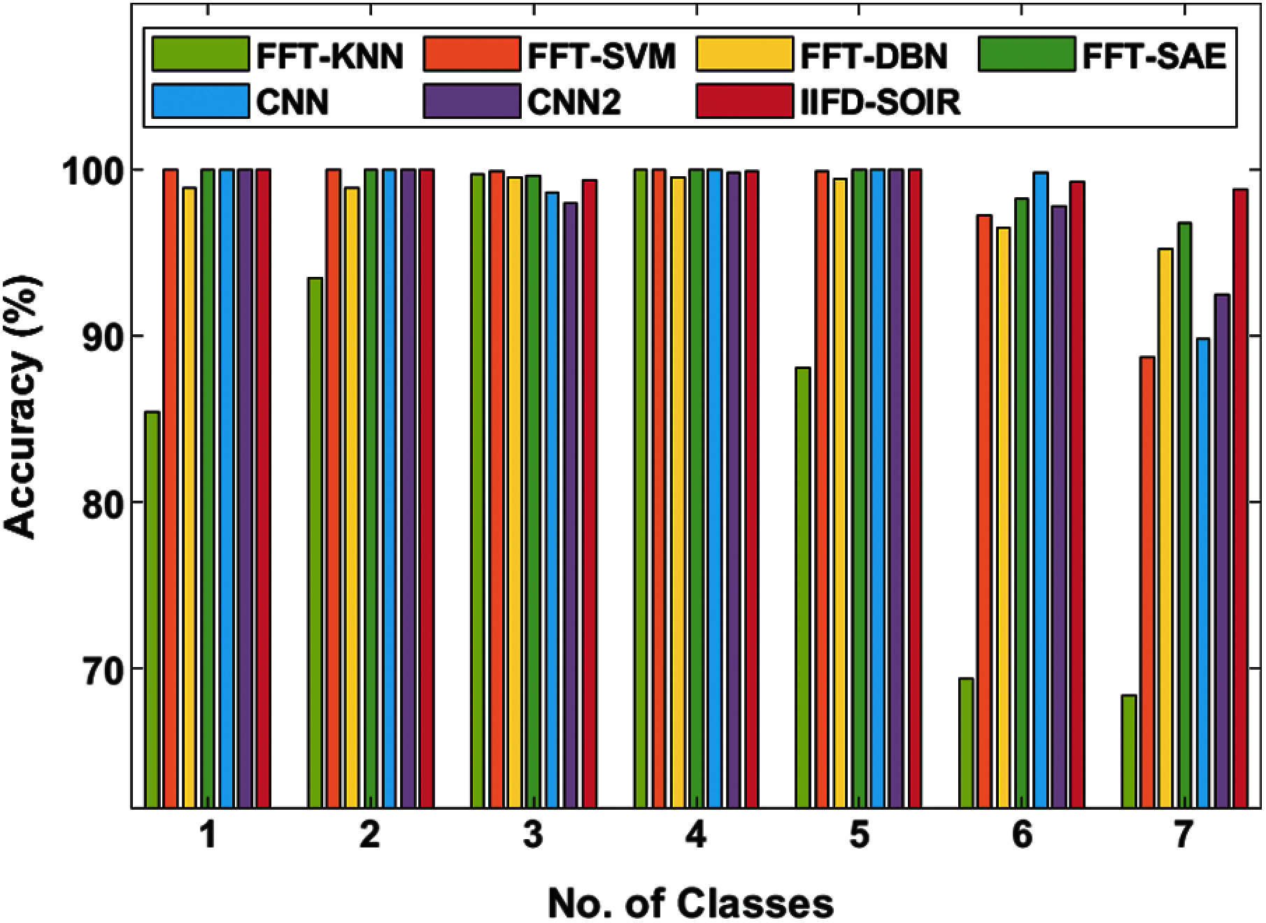
Figure 5: Accuracy analysis of IFD-SOIR approach on gearbox dataset

Average accuracy analysis of the IIFD-SOIR model with the existing models is also made. The experimental values stated that the FFT-KNN model has exhibited worse performance with the least average accuracy of 86.353%. At the same time, the FFT-SVM model has offered slightly better performance with an average accuracy of 97.956%. Followed by, the FFT-DBN, CNN2, and CNN models have appeared moderate and closer average accuracy of 98.271%, 98.289%, and 98.304% respectively. Though the FFT-SAE model has obtained a high average accuracy of 99.231%, the proposed IIFD-SOIR model has demonstrated superior performance with an average accuracy of 99.6%.

Fig. 6 examines the accuracy analysis of various fault classes by the IIFD-SOIR method on the applied Bearing dataset. On the given bearing dataset 1, the IIFD-SOIR, FFT-SVM, FFT-DBN, and FFT-SAE methodologies have gained higher accuracy of 99.82%, 100%, 100%, and 100% while the FFT-KNN, CNN, and CNN2 methods have showcased moderate function with the accuracy of 99%, 99.77%, 99.41% correspondingly. Similarly, on the applied bearing dataset 2, the IIFD-SOIR, FFT-DBN, FFT-SAE, and FFT-KNN approaches have achieved higher accuracy of 99.10%, 98.64%, 98.24%, and 97.72% whereas the FFT-SVM, CNN, and CNN2 methods have exhibited reasonable function with the accuracy of 96.56%, 95.87%, 93.24% respectively. In line with this, on the applied bearing dataset 3, the FFT-SVM, IIFD-SOIR, FFT-SAE, CNN, and CNN2 schemes have attained supreme accuracy of 100%, 100%, 100%, 100%, and 100% while the FFT-DBN and FFT-KNN schemes have illustrated acceptable function with the accuracy of 99.94% and 99% correspondingly. Meanwhile, on the applied bearing dataset 4, the FFT-SVM, IIFD-SOIR, CNN, and CNN2 technologies have accomplished the best accuracy of 99.57%, 99.45%, 99.26%, and 98.99% while the FFT-DBN, FFT-SAE and FFT-KNN approaches have depicted moderate function with the accuracy of 98.79%, 98.38%, 95.39% respectively. Then, on the applied bearing dataset 5, the IIFD-SOIR, CNN, FFT-SVM, and FFT-DBN technologies have attained higher accuracy of 99.81%, 99.72%, 99.30%, and 98.64% while the FFT-SAE, CNN2, and FFT-KNN techniques have illustrated considerable performance with the accuracy of 98.23%, 97.78%, 97.56% respectively.

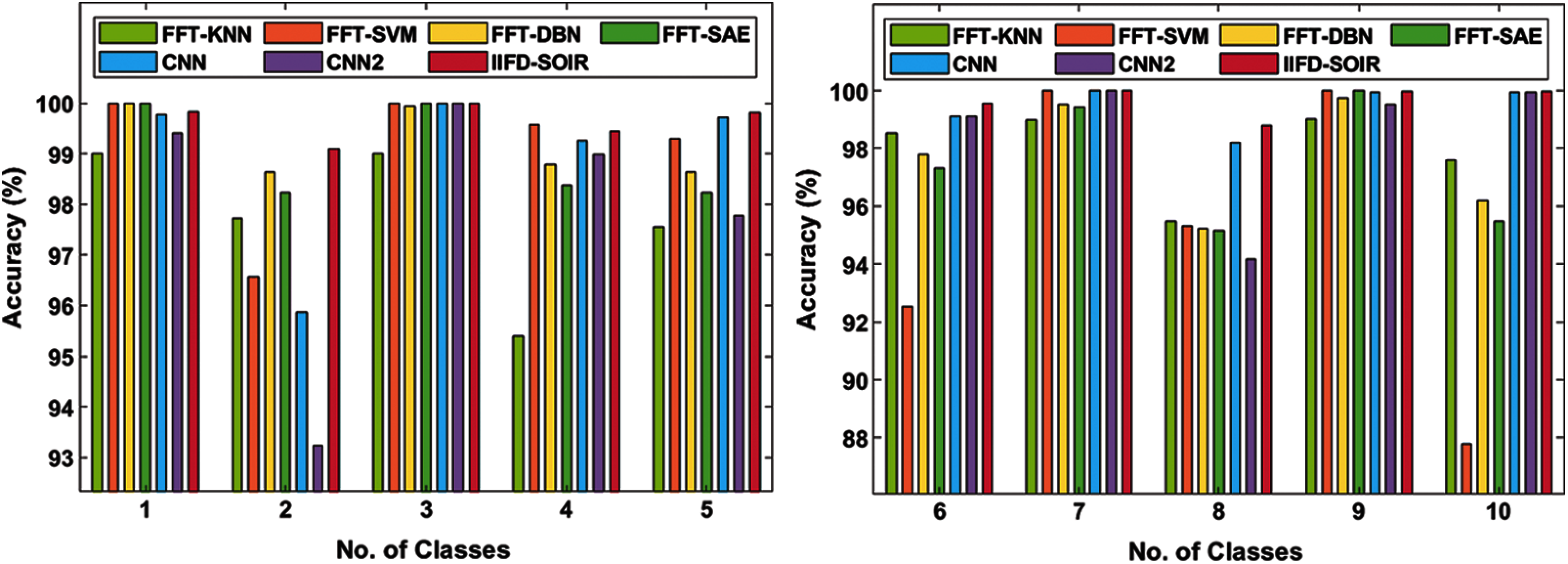
Figure 6: Accuracy analysis of IFD-SOIR approach on bearing dataset

In addition, on the applied bearing dataset 6, the IIFD-SOIR, CNN, CNN2, and FFT-KNN methods have accomplished high accuracy of 99.56%, 99.09%, 99.10%, and 98.53% while the FFT-SAE, FFT-DBN, and FFT-SVM frameworks have depicted reasonable performance with the accuracy of 97.32%, 97.78%, 92.52% correspondingly. In addition, on the applied bearing dataset 7, the IIFD-SOIR, FFT-SVM, CNN, and CNN2 methodologies have achieved superior accuracy of 100%, 100%, 100%, and 100% while the FFT-DBN, FFT-SAE, and FFT-KNN technologies have represented the least performance with the accuracy of 99.51%, 99.43%, 98.97% respectively. Followed by, on the applied bearing dataset 8, the IIFD-SOIR, CNN, FFT-KNN, and FFT-DBN schemes have obtained higher accuracy of 98.80%, 98.20%, 95.49%, and 95.22%, and the FFT-SVM, FFT-SAE, and CNN2 technologies have illustrated minimum performance with the accuracy of 95.31%, 95.15%, 94.18% correspondingly. Moreover, on the applied bearing dataset 9, the FFT-SVM, FFT-SAE, IIFD-SOIR, and CNN schemes have accomplished the best accuracy of 100%, 100%, 99.96%, and 99.94% whereas the FFT-DBN, CNN, and FFT-KNN techniques have exhibited considerable function with the accuracy of 99.76%, 99.94%, 99% respectively. Next, on the applied bearing dataset 10, the IIFD-SOIR, CNN, CNN2, and FFT-KNN frameworks have achieved the best accuracy of 99.97%, 99.94%, 99.94%, and 97.61% while the FFT-SVM, FFT-DBN, and FFT-SAE methods have depicted lower function with the accuracy of 87.80%, 96.19%, 95.49% respectively.

Average accuracy analysis of the IIFD-SOIR method with the previous approaches is also made. The experimental measures have revealed that the FFT-SVM technique has represented inferior function with the lower average accuracy of 97.106%. Simultaneously, the FFT-SVM technique has provided moderate function with an average accuracy of 97.827%. Besides, the FFT-DBN, FFT-SAE, and CNN2 methodologies have displayed considerable and closer average accuracy of 98.447%, 98.224%, and 98.084% correspondingly. Although the CNN approach has attained maximum average accuracy of 99.179%, the projected IIFD-SOIR framework has depicted a supreme function with an average accuracy of 99.647%.

Tab. 1 and Figs. 7 and 8 investigate the average accuracy analysis of the IIFD-SOIR model of the training and testing on the applied gearbox and Bearing dataset. On the applied gearbox dataset the FFT-KNN model has achieved the worst performance of an average training and testing accuracy of 90.84% and 86.35% respectively. Similarly, the FFT-SVM method achieved a moderate function of average training and testing accuracy of 98.58% and 97.95%, respectively, using a moderate function of average training and testing accuracy. According to this, the CNN2 technique has a higher average training and testing accuracy of 98.87% and 98.29%, respectively. Next, the CNN framework has obtained a reasonable function of average training and testing accuracy of 99.33% and 98.30% respectively. Simultaneously, the FFT-DBN framework has obtained moderate performance of average training and testing accuracy of 100% and 98.27% respectively. At the same time, the FFT-SAE approach has obtained maximum performance of average training and testing accuracy of 100% and 99.23% respectively. Moreover, the IIFD-SOIR scheme has achieved higher performance of average training and testing accuracy of 100% and 99.60% respectively.

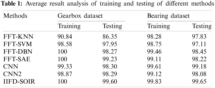
On the applied bearing gearbox dataset the FFT-KNN method has accomplished poor function of an average training and testing accuracy of 98.28% and 97.83% correspondingly. Likewise, the FFT-SVM approach has attained a moderate function of average training and testing accuracy of 98.75% and 97.11% respectively. In line with this, the FFT-SAE model has obtained maximum performance of average training and testing accuracy of 99.11% and 98.22% respectively. Then, the CNN2 technique has accomplished moderate performance of average training and testing accuracy of 99.12% and 98.08% correspondingly. Meanwhile, the FFT-DBN approach has attained the least function of average training and testing accuracy of 99.46% and 98.45% respectively. At the same time, the CNN framework has accomplished the maximum function of average training and testing accuracy of 99.61% and 99.18% respectively. Additionally, the IIFD-SOIR model has achieved optimal performance of average training and testing accuracy of 99.83% and 99.65% respectively. From the above-mentioned experimental values, it is evident that the IIFD-SOIR model has resulted in effective performance over the compared methods due to the following reasons. The employed IRV2 model achieves a faster training rate with certainly better accuracy over the Inception v4 model. Besides, the parameter tuning of the DL model using the SFO algorithm also plays a vital role in the improved classification performance.

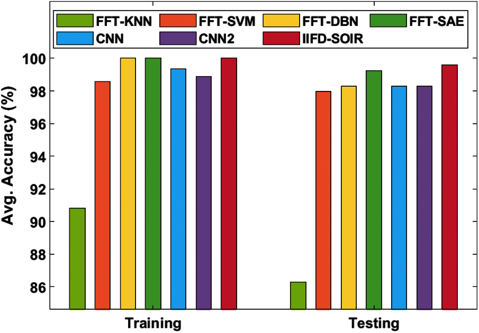
Figure 7: Average accuracy analysis of IIFD-SOIR model on gearbox dataset

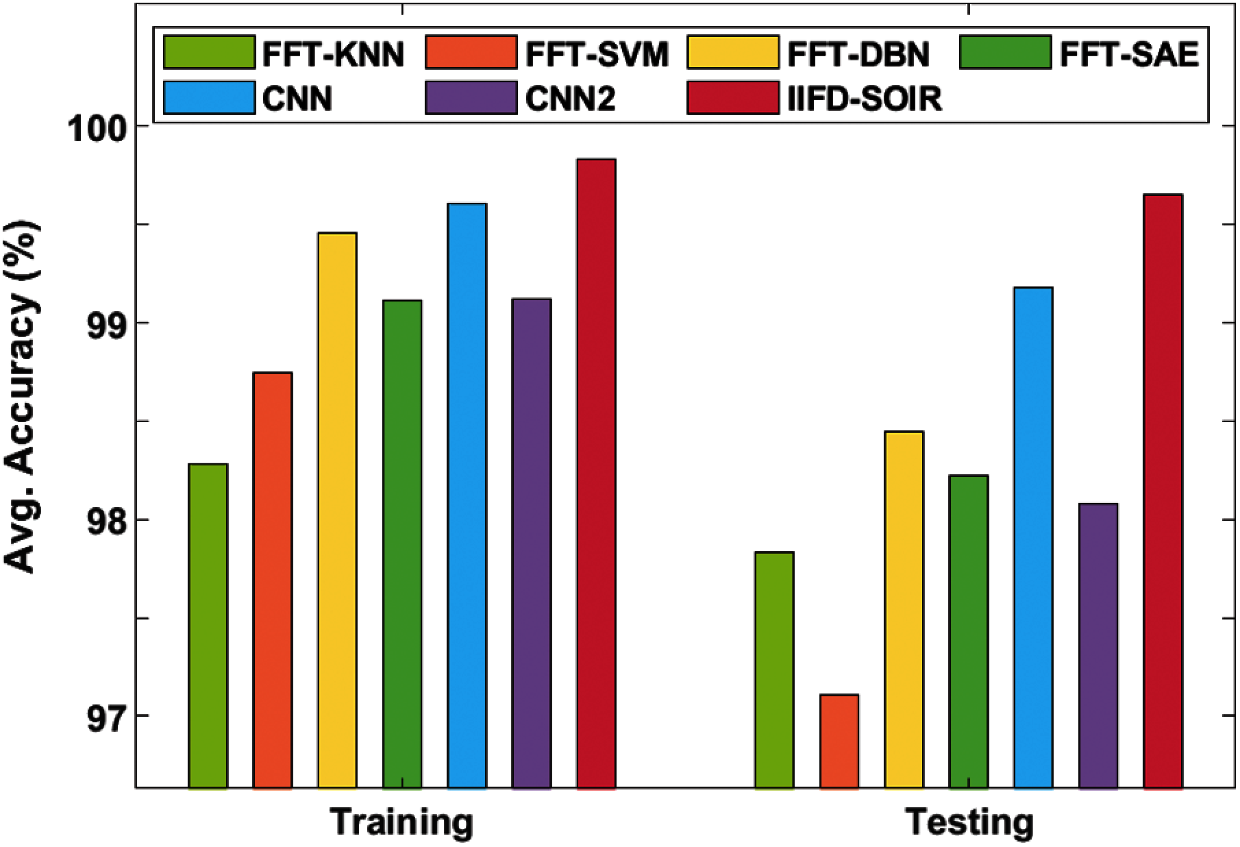
Figure 8: Average accuracy analysis of IFD-SOIR model on bearing dataset

5  Conclusion

This paper has developed an IIFD-SOIR model to identify faults in rotating machinery. Initially, the data acquisition process takes place to collect the data. Then, the CWTS model is applied to preprocess and crop the vibration signals. Followed by, the SFO algorithm tuned Inception with ResNet v2 model is applied as a feature extractor. The parameter tuning of Inception with the ResNet v2 model takes place using the SFO algorithm. Finally, MLP is applied as a classification model to identify the different kinds of faults. Extensive experimentation takes place to ensure the outcome of the IIFD-SOIR model on the gearbox dataset and a motor bearing dataset. The experimental outcome indicated that the IIFD-SOIR model has reached a higher average accuracy of 99.6% and 99.64% on the applied gearbox dataset and bearing dataset. The IIFD-SOIR model can be employed as an appropriate tool for diagnosing faults in rotating machienry. In the future, the IIFD-SOIR model can be employed in real-time industries for diagnosis faults.

Funding Statement: This research has been funded by Dirección General de Investigaciones of Universidad Santiago de Cali under call No. 01-2021. The authors would like to thank Chennai Institute of Technology for providing us with various resources and unconditional support for carrying out this study.

Conflicts of Interest: The authors declare that they have no known competing financial interests or personal relationships that could have appeared to influence the work reported in this paper.

This work is licensed under a Creative Commons Attribution 4.0 International License, which permits unrestricted use, distribution, and reproduction in any medium, provided the original work is properly cited.