Computers, Materials & Continua DOI:10.32604/cmc.2022.021978
Article

ATS: A Novel Time-Sharing CPU Scheduling Algorithm Based on Features Similarities

Samih M. Mostafa1,*, Sahar Ahmed Idris2 and Manjit Kaur3

1Faculty of Computers and Information, South Valley University, Qena, 83523, Egypt
2College of Industrial Engineering, King Khalid University, Abha, Saudi Arabia
3School of Engineering and Applied Sciences, Bennett University, Greater Noida, India
*Corresponding Author: Samih M. Mostafa. Email: samih_montser@sci.svu.edu.eg
Received: 22 July 2021; Accepted: 23 August 2021

Abstract: Minimizing time cost in time-shared operating systems is considered basic and essential task, and it is the most significant goal for the researchers who interested in CPU scheduling algorithms. Waiting time, turnaround time, and number of context switches are the most time cost criteria used to compare between CPU scheduling algorithms. CPU scheduling algorithms are divided into non-preemptive and preemptive. Round Robin (RR) algorithm is the most famous as it is the basis for all the algorithms used in time-sharing. In this paper, the authors proposed a novel CPU scheduling algorithm based on RR. The proposed algorithm is called Adjustable Time Slice (ATS). It reduces the time cost by taking the advantage of the low overhead of RR algorithm. In addition, ATS favors short processes allowing them to run longer time than given to long processes. The specific characteristics of each process are; its CPU execution time, weight, time slice, and number of context switches. ATS clusters the processes in groups depending on these characteristics. The traditional RR assigns fixed time slice for each process. On the other hand, dynamic variants of RR assign time slice for each process differs from other processes. The essential difference between ATS and the other methods is that it gives a set of processes a specific time based on their similarities within the same cluster. The authors compared between ATS with five popular scheduling algorithms on nine datasets of processes. The datasets used in the comparison vary in their features. The evaluation was measured in term of time cost and the experiments showed that the proposed algorithm reduces the time cost.

Keywords: Clustering; CPU scheduling; round robin; average turnaround time; average waiting time

1  Introduction

1.1 CPU Scheduling

CPU scheduling is defined as allocating and de-allocating the CPU to a specific process/thread. CPU scheduling is the most important and most effective task in the performance of the operating system [1–3]. CPU scheduling should provide efficient and fair usage of the computing resource (i.e., CPU time). The main goal of CPU scheduling is managing CPU time for running and waiting processes to provide the users with efficient throughput. The scheduler is the part of the OS that responsible to perform this task by choosing the next process to be allocated or de-allocated. The scheduling technique is divided into non-preemptive or preemptive. The non-preemptive technique does not suspend the running process until the process releases the CPU voluntarily. In contrast, under predetermined conditions, the preemptive technique suspends the running process. The task of choosing a process for execution is defined as scheduling and the algorithm used for this choice is indicated as the scheduling algorithm. Scheduling process described in Fig. 1 [4].

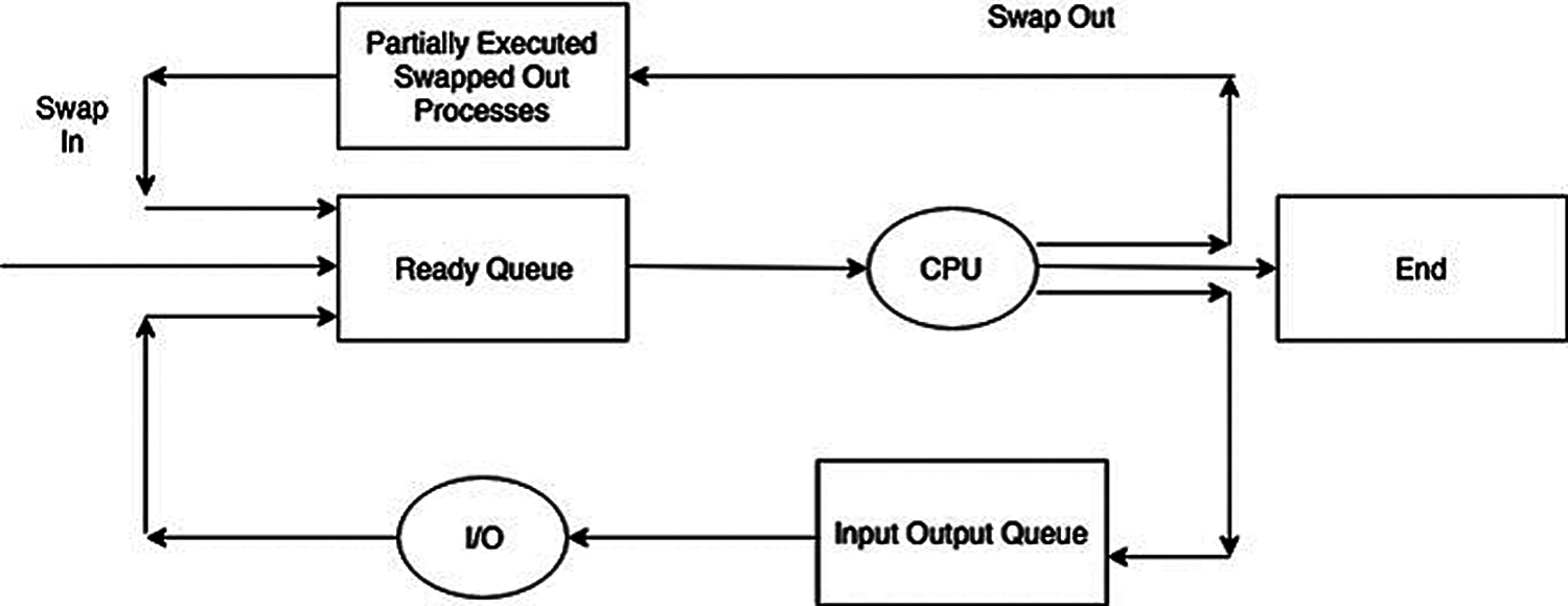
Figure 1: Schematic of scheduling

1.2 Scheduling Criteria

Different CPU scheduling algorithms have different characteristics and the choice of a specific algorithm influences the performance of the system, so the characteristics of the algorithms must be considered. For comparing between CPU scheduling algorithms, many scheduling criteria have been suggested (i.e., waiting time (WT), turnaround time (TT) and number of context switches (NCS)). WT is the sum of the periods that the processes spent waiting in the ready queue. TT is the interval from the submission time of a process to the completion time. NCS is the number of times the process is stopped, put at the tail of the queue to be resumed. The scheduler executes the process at the head of the queue. The scheduler is considered efficient if it minimizes WT, TT, and NCS.

1.3 Basic Scheduling Algorithm

1.3.1 First Come First Serve (Non-Preemptive Scheduler)

The easiest and the simplest non-preemptive CPU scheduling algorithm is the First come First Serve (FCFS) algorithm. The policy of FCFS implementation is managed with a FIFO queue in which the process that arrives to the ready queue first is assigned to the CPU first (see Fig. 2).

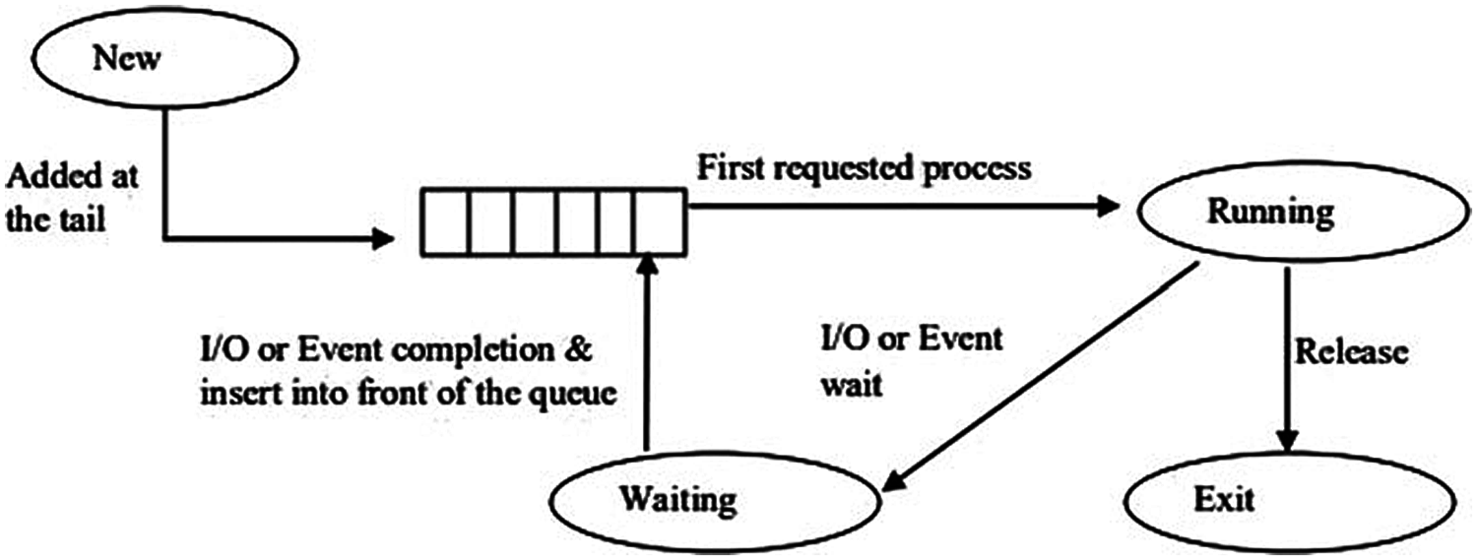
Figure 2: FCFS CPU scheduling

1.3.2 Shortest Job First (Non-Preemptive Scheduler)

In the Shortest Job First (SJF), the CPU is assigned to the process with the smallest burst time. SJF compares between the burst times of all processes residing in the ready queue and selects the process with the smallest burst time. If two processes have the same burst times, FCFS scheduling is used (see Fig. 3).

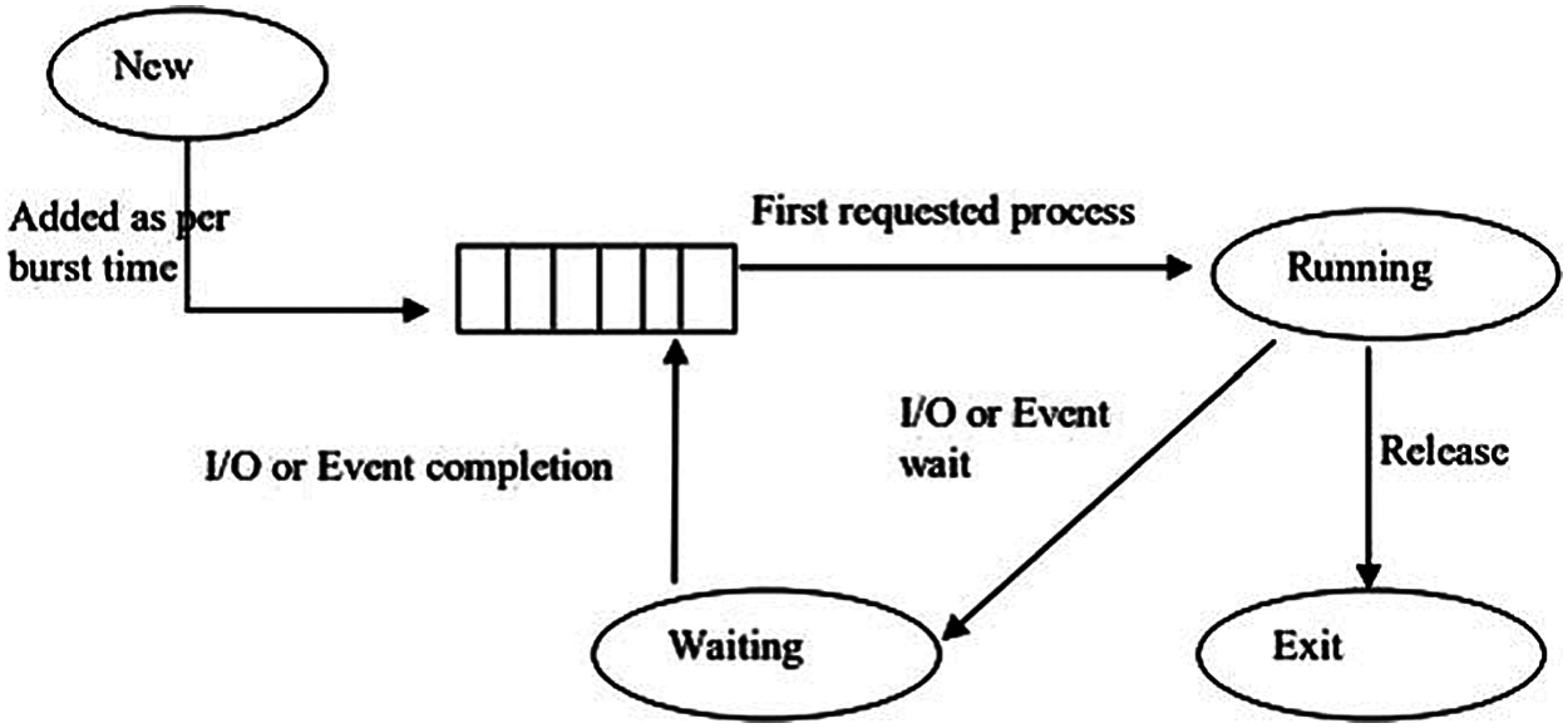
Figure 3: SJF CPU scheduling

1.3.3 Round Robin Scheduling

Round Robin scheduling (Fig. 4) allocates each process an equal portion of the CPU time. The policy of RR implementation is managed with a FIFO queue. Processes are in a circular queue; the process is put to the tail of the queue and the selected process for execution is taken from the front [5].

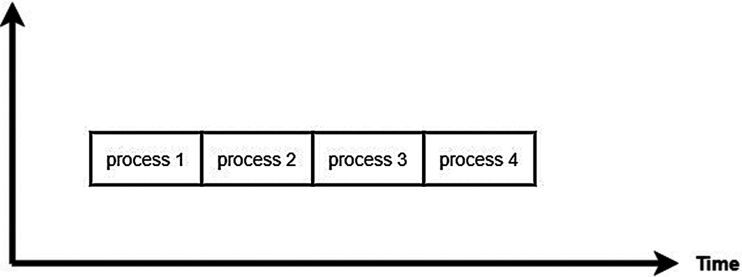
Figure 4: Round robin scheduling

The OS is driven by an interrupt (i.e., clock tick). Processes are chosen in a fixed sequence for execution. On each clock tick, the process running is paused and the next process starts execution. All processes wait in the queue for the slot of CPU time where all of them are treated as of equal importance. Process is not permitted to run to completion, but it is preempted. The implications of the preemptive process switching and the overhead are significant and must be taken into consideration. There is an inescapable time overhead when the process and context are switched (represented by the black bars in Fig. 5).

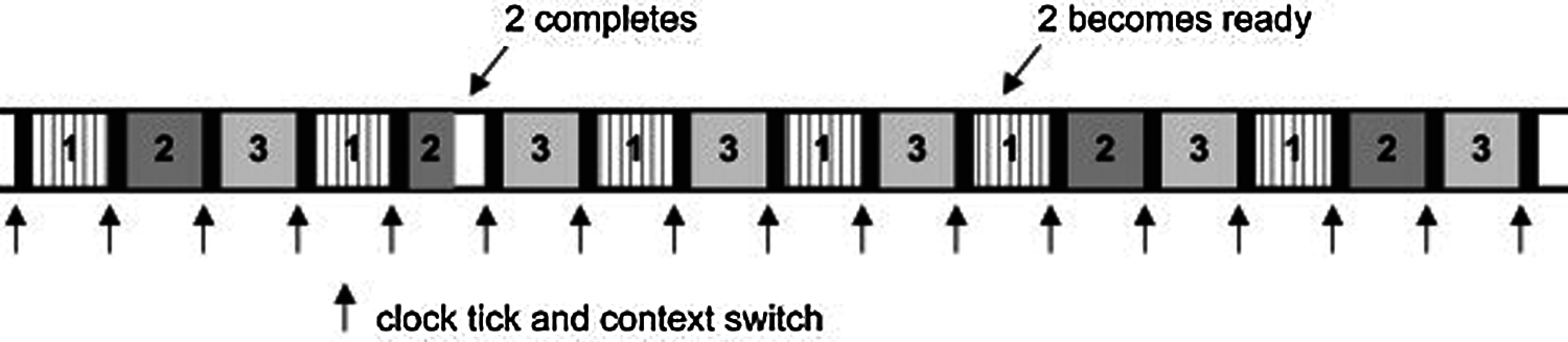
Figure 5: Context switches overhead

For example, assume that the scheduler runs three processes {A, B, C} in the sequence A, B, C, A, B, C, A, …., until they are all completed. This sequence for these processes is shown in Fig. 6. It is noticed that the processor is busy all the time because there is a process is running. The pseudocode of the RR algorithm is shown in Algorithm 1.

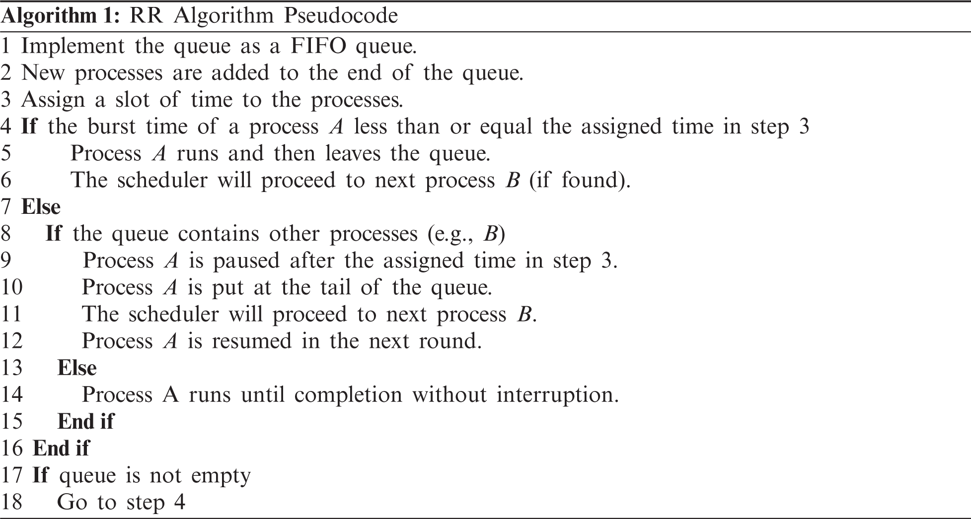
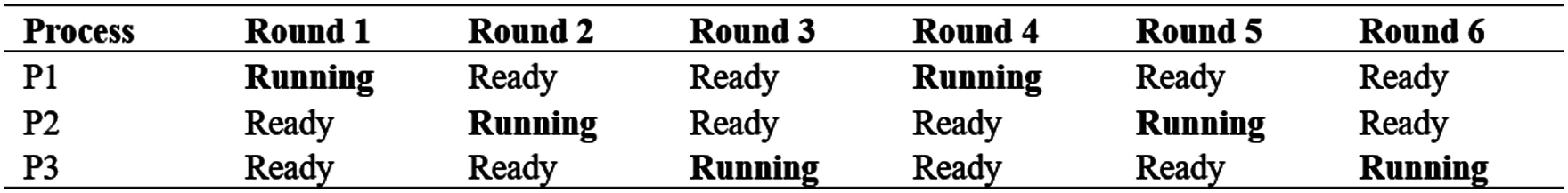
Figure 6: A sequence of process state for RR scheduling with three processes

1.4 Clustering Technique

Dividing the data into useful, meaningful, or both is known as clustering [6]. The greater the difference between the clusters and the greater the similarity between the elements within the same cluster, the better the clustering [7]. Both clustering and classification are fundamental tasks in machine learning. Clustering is used mostly as an unsupervised learning, and classification for unsupervised learning. The goal of classification is predictive, and that of clustering is descriptive which means that the target of clustering is to find out a new set of groups, the assessment of these groups is intrinsic and they are of interest in themselves. Clustering gathers data elements into subsets that similar elements are grouped together, while different elements belong to different groups [8,9]. The categorization process is determined by the selected algorithm [7]. Features’ types determine the algorithm selected in the clustering (e.g., statistical algorithms for numeric data, conceptual algorithms for categorical data, or fuzzy clustering algorithms that allow data element to be joined to all clusters with a membership degree from 0 to 1). Most commonly used clustering algorithms are divided into traditional and modern clustering algorithms [10].

1.4.1 K-means Clustering Algorithm

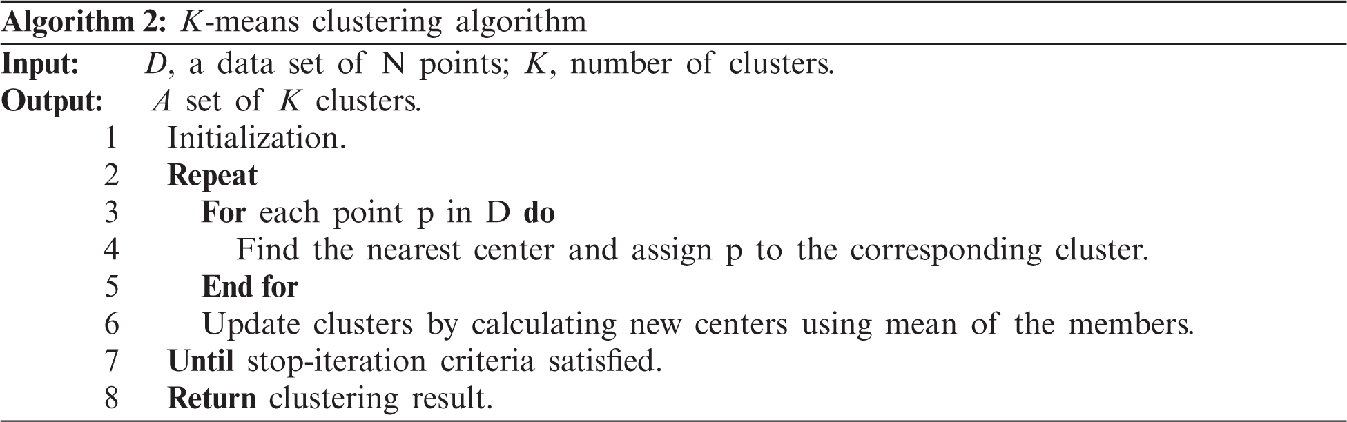
K-means is the most common of clustering algorithms, the steps of K-means are shown in algorithm 2. The simplicity of K-means comes from the use of the stopping criterion (i.e., squared error). Suppose that D be the number of dimensions, N the number of elements, and K the number of centers, and K-means runs I iterations, hence K-means time complexity is O(NKI). The goal of K-means is to minimize some objective function which is described in Eq. (1) [11].

min{mk},1≤k≤K∑k=1K⁡∑x∈Ck⁡πxdist(x,mk)(1)

where K is the number of the clusters, πx is the weight of x, mk=∑x∈Ck⁡πxxnk is the centroid of cluster Ck, The distance between centroid and the object x is computed by the function ‘dist’, 1≤k≤K. Determining the number of clusters k is discussed in the next subsection.

1.4.2 Silhouette Method

Silhouette method is one of the most popular clustering evaluation techniques. It determines how well each element lies within its cluster, so it measures the clustering quality. It can be summarized as follows:

(1)   Applying the selected clustering algorithm for different values of k.

(2)   Calculating the Within-cluster Sum of Square (WSS) for each k.

(3)   Plotting WSS curve.

(4)   The knee's position in the curve points out the suitable number of clusters.

Eq. (2) defines the Silhouette coefficient (Si) of the ith data point.

Si=biaimax(bi,ai)(2)

where bi is the average distance between all elements in different clusters and the ith element; ai is the average distance between all elements in the same cluster and the ith element [12,13]. Fig. 7 shows the organization of the paper.

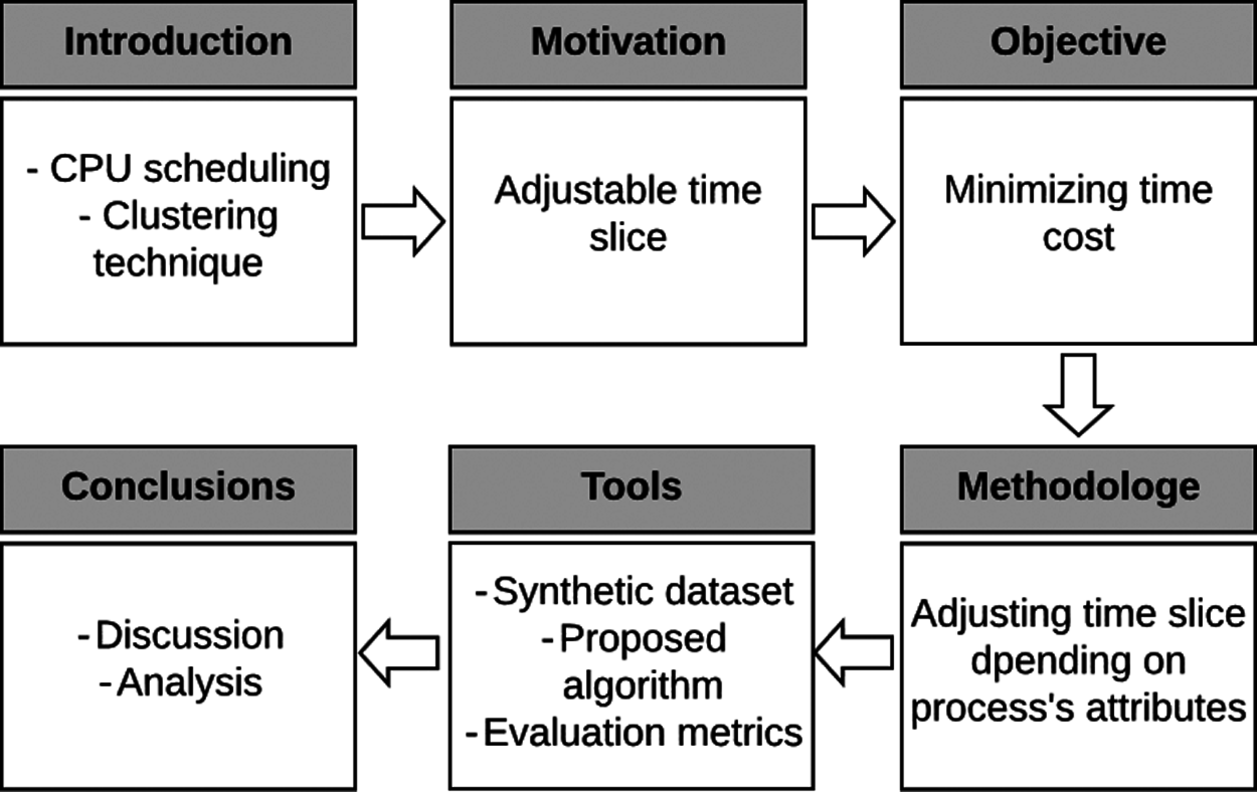
Figure 7: Organization of the paper

2  Related Works

Various forms of the RR algorithm have been proposed to minimize time cost. This section shows the most common of these forms. Tab. 1 compares between these versions of RR. Harwood et al. [14] proposed VTRR (Variable Time Round-Robin scheduling) algorithm which is a dynamic form of RR algorithm. VTRR takes into consideration the time needed to all processes when assigning the time slice to a process. Tarek et al. proposed BRR (Burst RR) a weighting form of RR by grouping five groups of processes and each process belongs to a group depending on its burst time. The weight of each process is inversely proportional to its burst time [15]. Mostafa et al. [16] proposed CTQ (Changeable Time Quantum), CTQ finds the time slice that gives smallest waiting time and turnaround time and every process runs for that time. Mishra et al. [17] proposed IRRVQ (improved Round Robin with varying time quantum) in which the processes are sorted in ascending order and the queue is divided into heavy and light. The time slice in each round is equal to the median processes’ burst time. On a similar approach, Lipika proposed a dynamic form of RR, the time slice is calculated at beginning of each round depending on the residual burst times of the processes in the successive rounds, the processes are sorted in ascending order [18]. McGuire et al. [19] proposed Adaptive80 RR, the time slice equals the burst time of the process at 80th percentile. In the same way that Lipika took, Adaptive80 RR sorts the processes in ascending order. Samir et al. proposed SRDQ (SJF and RR with dynamic quantum), SRDQ divided the queue into Q1 (for short processes) and Q2 (for long processes; the process with burst time long than the median is considered long and the process with burst time small than the median is considered short. Like Lipika's and Adaptive80 RR, SRDQ sorts the processes in ascending order [20]. Mostafa [21] proposed PWRR (Proportional Weighted Round Robin) in which the burst time of a process is divided by the summation of all burst times and the time slice is assigned to a process based on its weight. Mostafa et al. [22] proposed ARR (Adjustable Round Robin) in which the short process is given a chance for completion without pausing, this is done under a predefined condition. In the same way, Uferah et al. proposed ADRR (Amended Dynamic Round Robin) in which the time slice is assigned to the process based on its burst time. Like some of its predecessors, ADRR sorts the processes in ascending order [23]. Samih et al. proposed DRR (Dynamic Round Robin) which uses clustering technique in grouping similar processes in a cluster, it differs from its predecessors in that it allocates time for the cluster and all processes get the same time within the same cluster [7]. Mostafa et al. [24] proposed DTS (Dynamic Time Slice), DTS takes the same approach as DRR in clustering the processes using K-means clustering technique, the only difference between them is the method of calculating the time slice.

3  Proposed Algorithm

Before starting the proposed algorithm, the meanings of abbreviations used should be clarified as shown in Tab. 2.

The process features PW, PTQ, PBT, and NCS basically depend on BT. Firstly, the proposed approach rounds up similar processes in clusters and the resemblance between processes depends on these features. ATS algorithm uses k-means in the clustering process. Preparation of the data, clustering the data, and the dynamic implementation are the three stages of the proposed work, which are described in the following subsections.

3.1 Data Preparation

PW and NCS are calculated in this stage. Eq. (3) calculates PW, and Eq. (4) calculates NCS.

PWi=BTi∑j=1N⁡BTj(3)

where BTi is burst time of the ith process, N is the number of the processes.

NCSi={[BTiFTS]ifBTi≠h×FTSh=1,2,3,…BTiFTS−1ifBTi=h×FTSh=1,2,3,…(4)

FTS is determined by TRR algorithm (i.e., FTS that will be used to calculate the dynamic time slice is determined by the RR in the OS). ⌊X⌋ means the largest integer smaller than or equal to X. PTS changes from one process to another within the same round, and it changes from one round to another. The PTQ assigned to a process in a round is calculated from Eq. (5).

PTQi={FTSifBTi>FTSBTiifBTi≤FTS(5)

PBT of a process in a round is calculated from Eq. (6).

PBTi=BTi∑z=1n⁡PTQz(6)

PTS is calculated from Eq. (7).

PTSi=(1−PBTi)×FTS(7)

3.2 Data Clustering

The mean reason of choosing K-means clustering algorithm in this work is that K-means works properly only with the numerical features [9]. The parameter k is determined using Silhouette method, and k-means creates k clusters of data points. BT, PW, PTQ,PBT and NCS are the features used in the clustering. The cluster is represented by the centroid within this cluster. K-means is a gradient-decent procedure starts with an initial set of K cluster-centers and consecutively updates this set. Fig. 8 displays how K-means cluster a dataset (e.g., d31 dataset) [25].

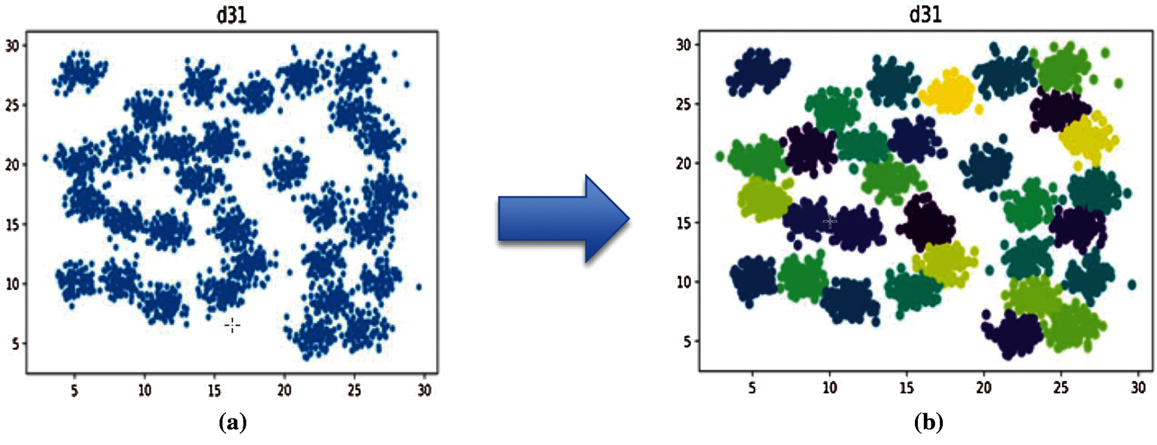
Figure 8: Clustering dataset using K-means A) d31 dataset before clustering B) d31 dataset after clustering

3.3 Dynamic Implementation

Process with long burst time causes more overhead resulted from numerous NCS. A threshold is predetermined to avoid this overhead. The proposed algorithm allows the process that close to finish to be completed and leave the queue. CWl (i.e., weight of the lth cluster) is computed from Eq. (8) and CTSl is computed from Eq. (9).

CWl=Cavgl∑m=1k⁡Cavgm(8)

CTSl=(1−CWl∑l=1k⁡CWl)×FTS(9)

The proposed algorithm behaved similar to the DTS algorithm [24] which takes into consideration not only the burst time of the process in the current round, but also the in the successive rounds. In addition, the proposed algorithm splits the queue into Q1 for short processes (shorter than median) and Q2 for long processes (longer than median) [20]. The proposed algorithm assigns each process with a time slice computed from Eq. (10).

ATSr,l={CTSl+threshold{if(threshold×(BTrFTS+1)≥mod(BTr,CTS))andif(BTr<Median)wheremod(BTr,CTS)>0CTSl{ifmod(BTr,CTS)=0andif(BTr≥Median)(10)

where ATSr,l is the adjustable time slice assigned to the process Pr in the cluster l. In consecutive rounds, RBT is updated according to Eq. (11). The proposed algorithm is described in Fig. 9.

RBTi=BTi−CTSi(11)

4  Experimental Implementation

The computer's specifications used in the experiments are shown in Tab. 3:

4.1 Benchmark Datasets

Nine artificial datasets were generated to be used in the experiments. Each dataset has a number of processes varying in the BTs which have been randomly generated. To prove that the proposed algorithm is valid for diverse data, each dataset contains different number of processes varying in their burst times and accordingly the PW, NCS, PTQ, PBT, and PTS are different. Tab. 4 presents the characteristics of the datasets used.

4.2 Performance Evaluation

The proposed algorithm has been compared with five common algorithms VTRR, DTS, ADRR PWRR and RR. The submitted processes may be arrived in the same time or different times. The experiments were conducted taking into account the two cases.

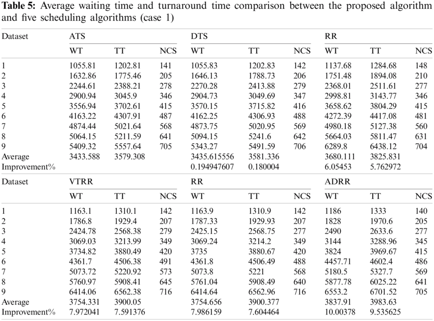
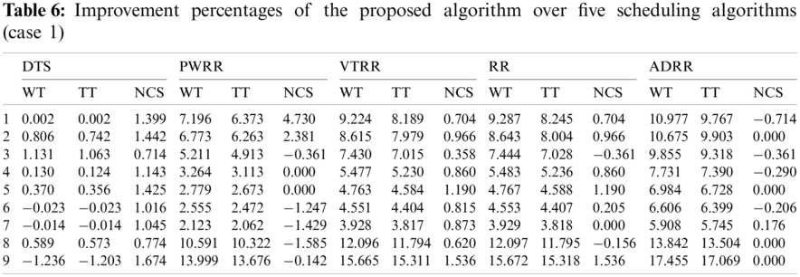
Case 1 (same arrival time): The average turnaround times and waiting times comparisons are shown in Fig. 10, the NCS comparisons are shown in Fig. 11. The improvement of ATS over the compared algorithms is shown in Fig. 12. Time cost comparisons are shown in Tab. 5 and the improvement is shown in Tab. 6.

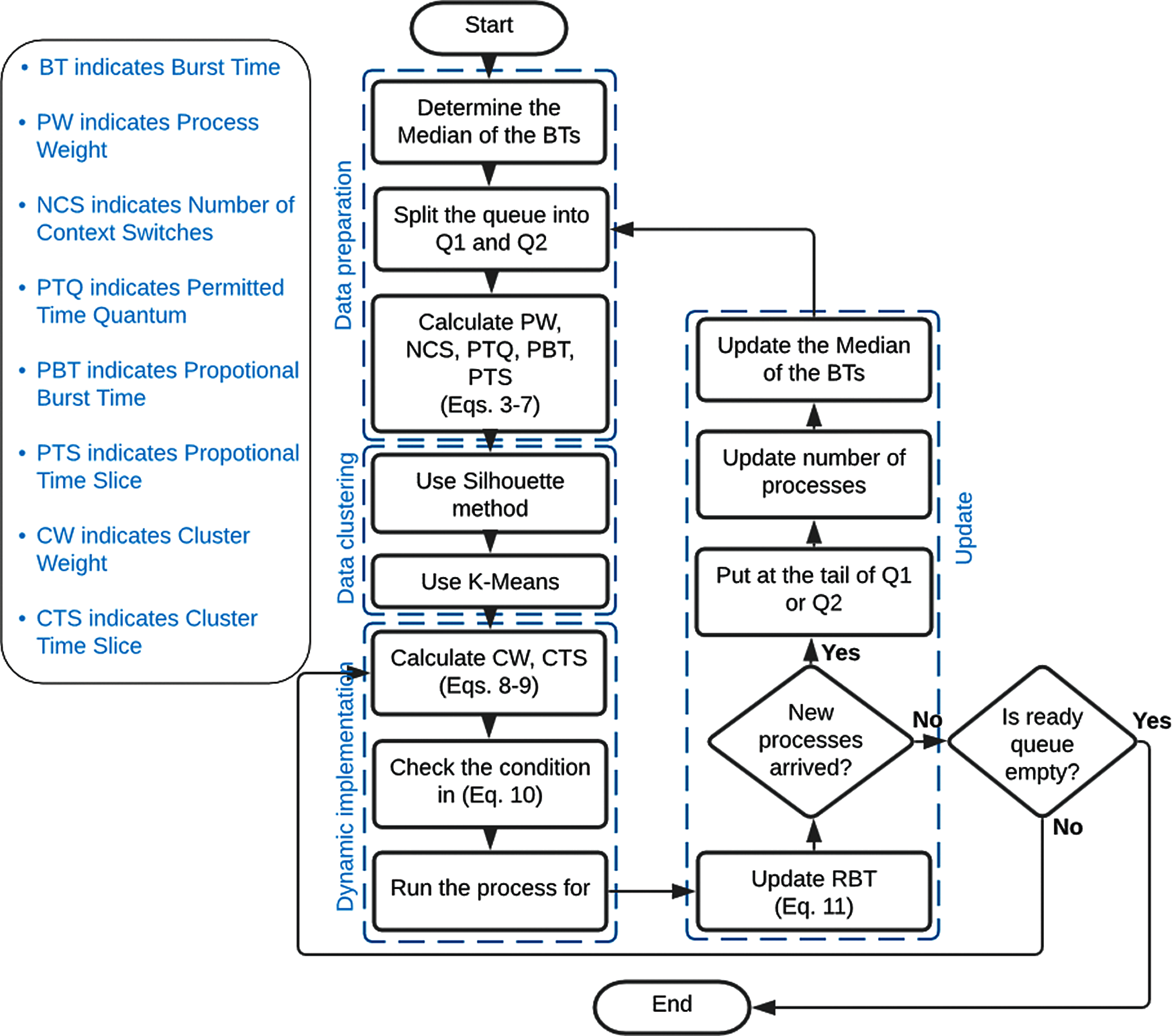
Figure 9: Algorithm flowchart

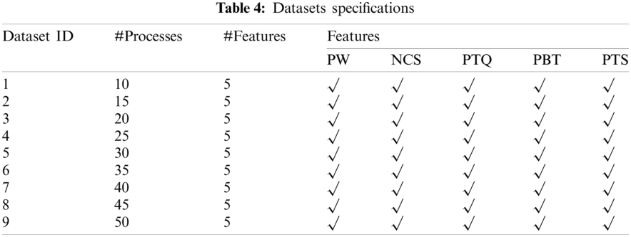
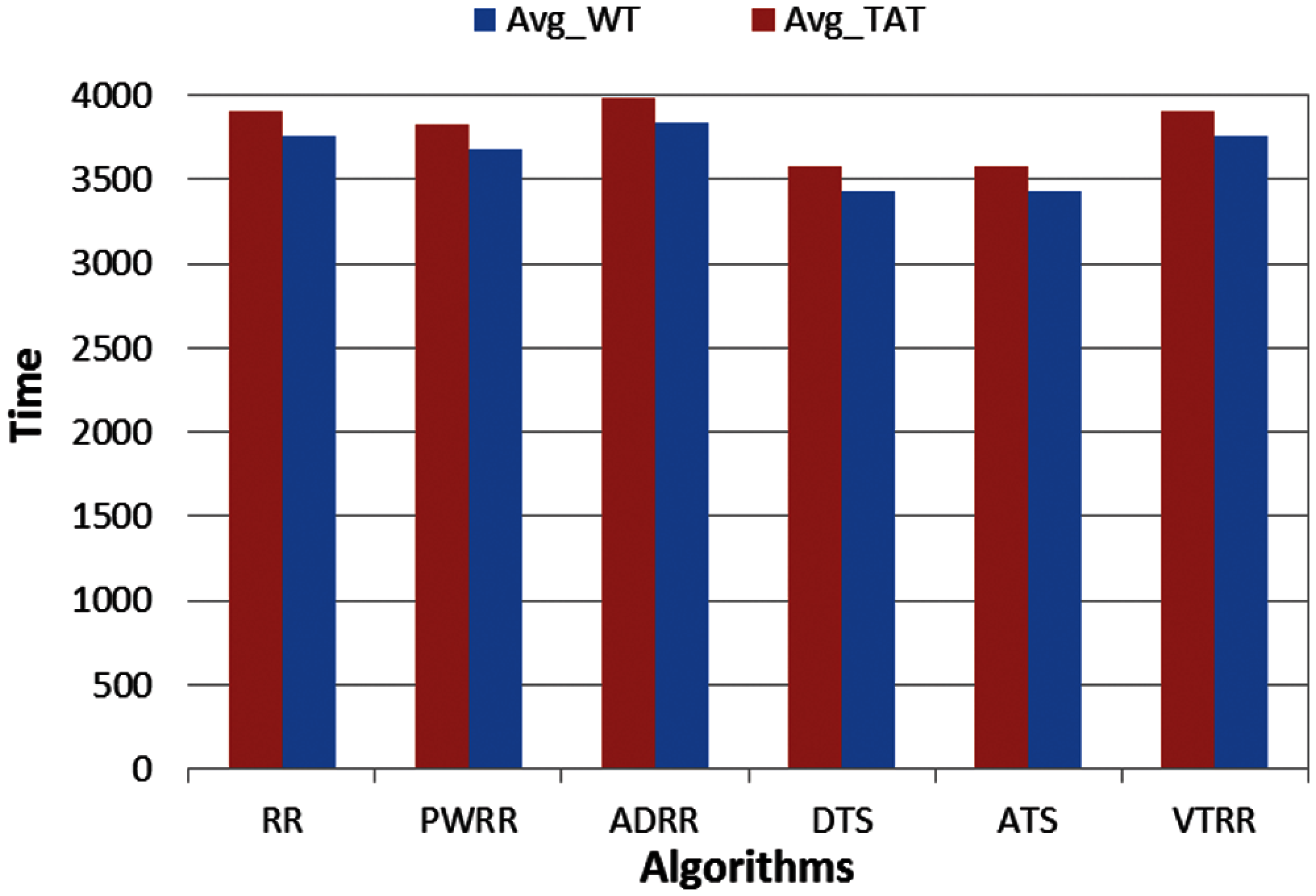
Figure 10: Avg_WT and Avg_TAT comparison (case 1)

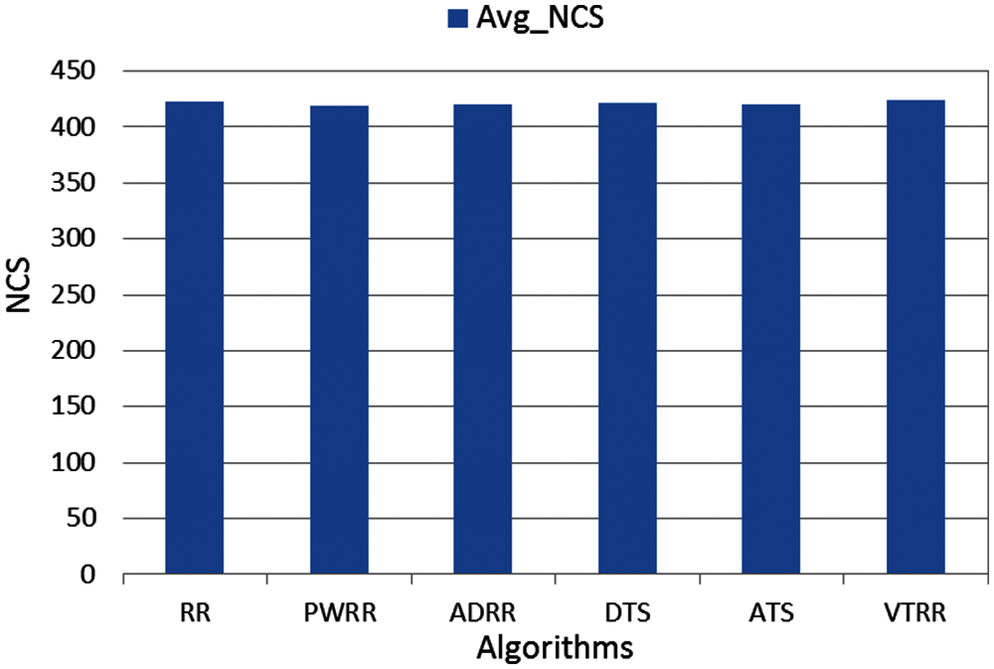
Figure 11: NCS comparison (case 1)

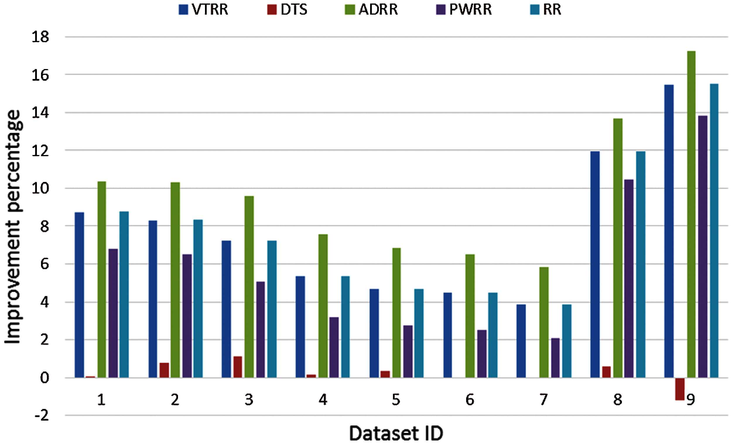
Figure 12: Improvement comparison (case 1)

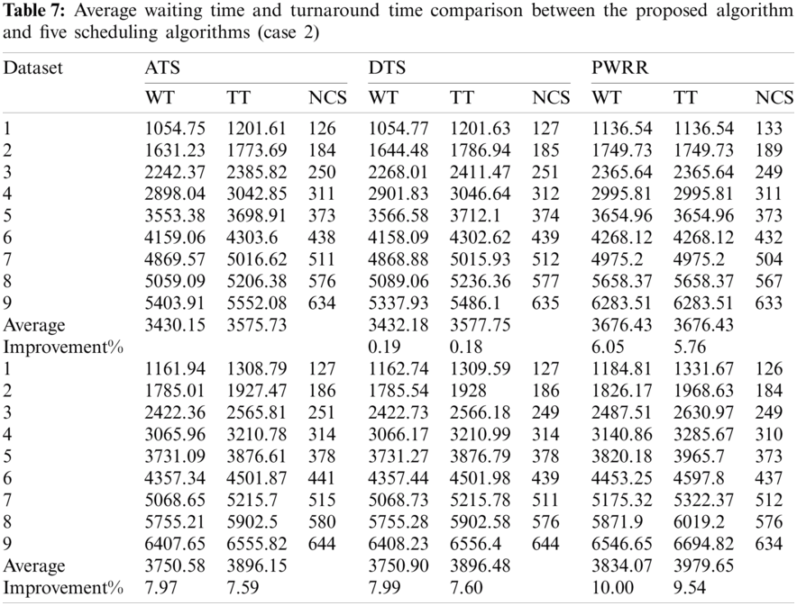
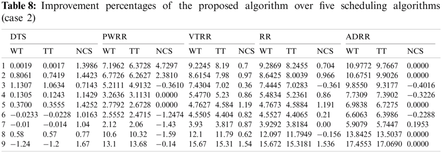
Case 2 (different arrival time): Process arrival was modeled as Poisson random process. The arrival times are exponentially distributed [16]. The average turnaround times and waiting times comparison are shown in Fig. 13, the NCS comparisons are shown in Fig. 14. The improvement of ATS over the compared algorithms is shown in Fig. 15. Time cost comparisons are shown in Tab. 7 and the improvement is shown in Tab. 8.

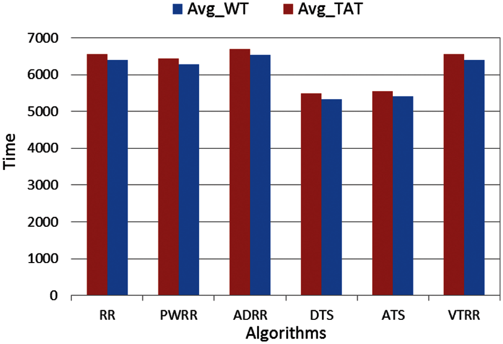
Figure 13: Avg_WT and Avg_TAT comparison (case 2)

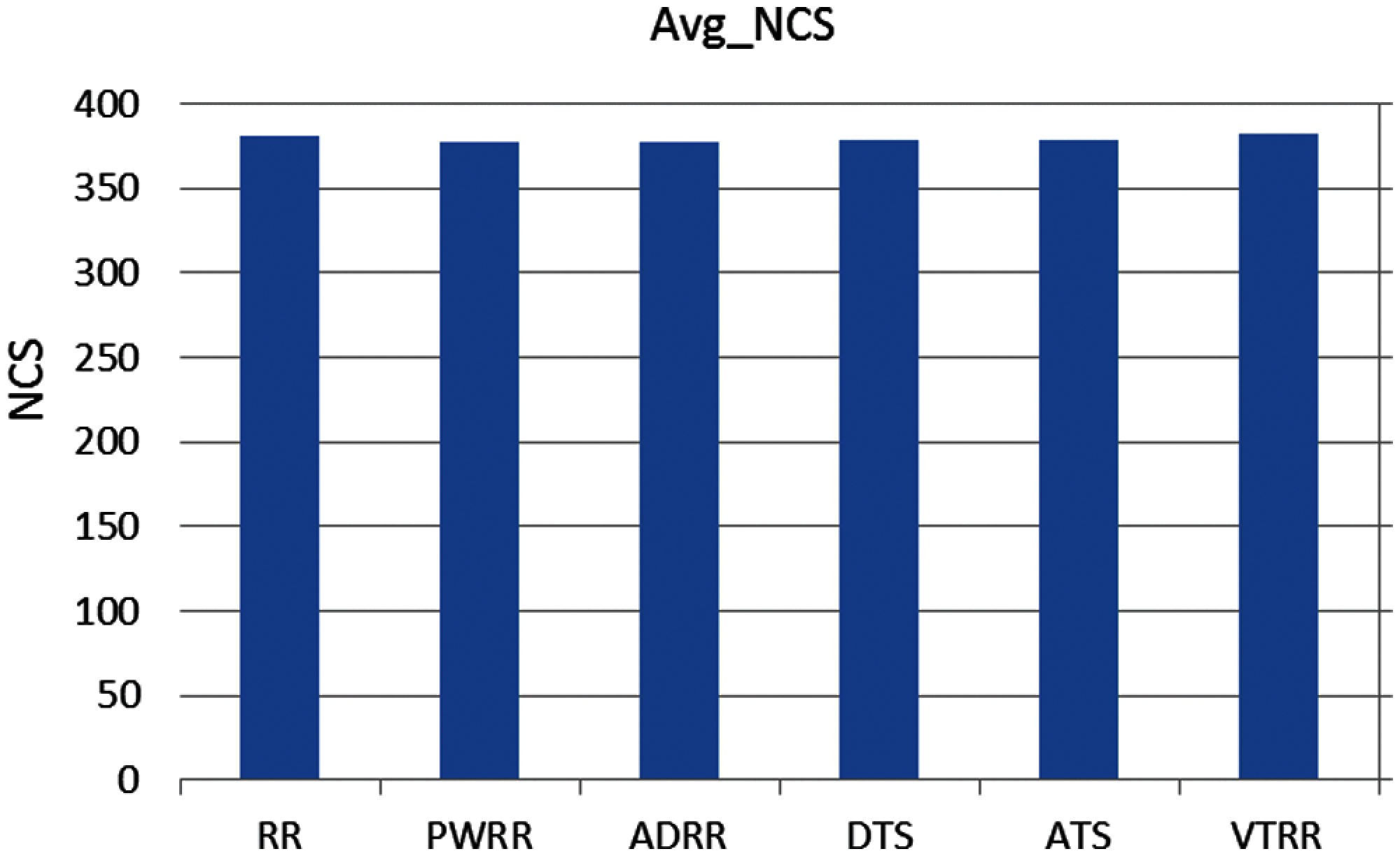
Figure 14: NCS comparison (case 2)

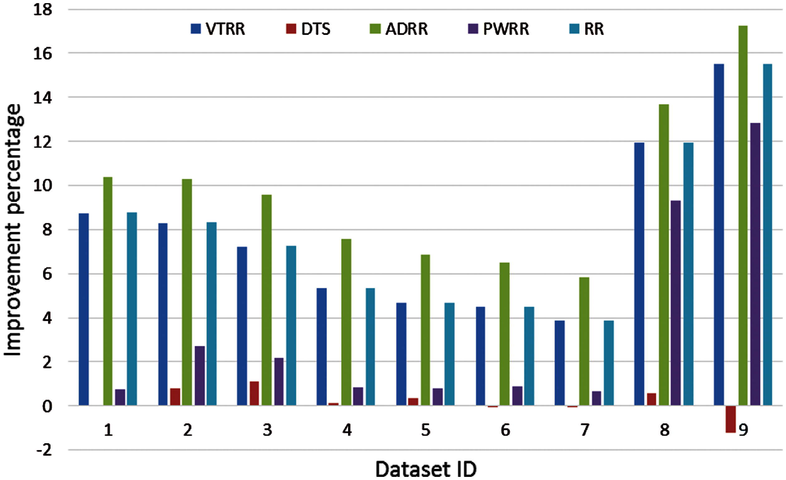
Figure 15: Improvement comparison (case 2)

5  Conclusion

This paper presented a dynamic version of RR. The proposed goal is to reduce the time cost (i.e., waiting time and turnaround time). The traditional RR uses fixed slot of time for each process in all rounds regardless the BT of the process, however, the proposed algorithm (ATS) assigns particular time slice for each process. This time slice is different from the other processes in the same cluster. If the BT of a process is longer than the assigned time slice, the process will be put at the end of the queue and assigned a new time slice in the new round. In addition, the proposed algorithm starts by grouping similar processes in a group depending on the similarity between the features. Each cluster is a signed a slot of time and every process in this cluster is assigned this time slice. In a round, some processes may finish their BT and leave the queue, and may new processes arrive. In both cases the number of the clusters and clusters’ weights will be updated and therefore the time slice assigned to a cluster and the number of the processes in the cluster will be updated. Furthermore, ATS takes into account the remaining times of the survived processes and allow short process to complete (under predetermined conditions) without interruption even if its BT longer than the assigned Time Slice, in other words, ATS grants more time to the process that is close to complete in the current and consecutive rounds. Comparison has been done between ATS and five common versions of RR from the point of view of time cost. The results showed that the proposed algorithm achieves noticeable improvements.

Funding Statement: The authors extend their appreciation to Deanship of Scientific Research at King Khalid University for funding this work through the Research Groups Project under Grant Number RGP.1/95/42.

Conflicts of Interest: The authors declare that they have no conflicts of interest to report regarding the present study.

This work is licensed under a Creative Commons Attribution 4.0 International License, which permits unrestricted use, distribution, and reproduction in any medium, provided the original work is properly cited.