DOI:10.32604/cmc.2022.020098
| Computers, Materials & Continua DOI:10.32604/cmc.2022.020098 | |
| Review |
Optimization of Reliability–Redundancy Allocation Problems: A Review of the Evolutionary Algorithms
1College of Engineering, Muzahimiyah Branch, King Saud University, Riyadh, 11451, Saudi Arabia
2University of Monastir, LGM, ENIM, Avenue Ibn-Eljazzar, 5019, Monastir, Tunisia
*Corresponding Author: Omar Al-mutiri. Email: 437170093@student.ksu.edu.sa
Received: 09 May 2021; Accepted: 25 June 2021
Abstract: The study of optimization methods for reliability–redundancy allocation problems is a constantly changing field. New algorithms are continually being designed on the basis of observations of nature, wildlife, and humanity. In this paper, we review eight major evolutionary algorithms that emulate the behavior of civilization, ants, bees, fishes, and birds (i.e., genetic algorithms, bee colony optimization, simulated annealing, particle swarm optimization, biogeography-based optimization, artificial immune system optimization, cuckoo algorithm and imperialist competitive algorithm). We evaluate the mathematical formulations and pseudo-codes of each algorithm and discuss how these apply to reliability–redundancy allocation problems. Results from a literature survey show the best results found for series, series–parallel, bridge, and applied case problems (e.g., overspeeding gas turbine benchmark). Review of literature from recent years indicates an extensive improvement in the algorithm reliability performance. However, this improvement has been difficult to achieve for high-reliability applications. Insights and future challenges in reliability–redundancy allocation problems optimization are also discussed in this paper.
Keywords: Reliability; redundancy; evolutionary algorithms
Continuous advancements in technology combined with the expectation for high performance by manufacturers and consumers add increasing complexity to modern manufactured systems. However, human errors during utilization (e.g., processing error, improper storage, poor equipment maintenance, or environmental impact) negatively affect the global performance and the designed life cycle of a manufactured system. Thus, system reliability is an important concern when designing and improving the efficiency of any engineering system. Reliability is defined as the likelihood of effectively achieving a set of functionality goals or product functions within a specified timeframe and in a regulated environment, even given uncertainty and inadequate knowledge of system actions.
System reliability design problems are divided into three categories: redundancy allocation problems, reliability allocation problems, and reliability–redundancy allocation problems (RRAPs). Common elements for all of these include decision variables, constraints, and objective function(s). Decision variables represent factors that can be altered or decisions that can be made to enhance system reliability. Constraints are factors that limit design, such as price, volume, weight, and reasonable specified reliability. An objective function(s) calculates the overall reliability function on the basis of defined values for the decision variables that comply with constraints of the optimal solution. The objective function may consist of a single function (e.g., system reliability to be maximized) or multiple functions (e.g., adding system costs while needing to minimize system volume).
System reliability optimization techniques evolved during the first half of the 20th century to support developments in mathematics, computing capabilities, optimization methodologies, system complexity, design, and management requirements [1–6]. Originally, these techniques applied the application of advanced mathematics to produce optimal solutions from equations that could be solved analytically. This limited the size and complexity of the studied problems. The invention of the computer greatly increased the number and types of mathematical approaches and allowed the handling of large datasets. The fields of dynamic programming [3], linear programming [7], nonlinear programming [8], and integer programming [9] were born. These mathematical approaches were needed because reliability problems are often highly nonlinear because of a nonlinear objective function(s) and the type of decision variable (continuous or integer).
The first use of dynamic programming to solve reliability problems was done for redundancy allocation problems [3,10,11]. This early work was very simplified with only a single component choice for each subsystem and a goal of maximizing reliability from a single cost constraint. The issue for each subsystem was to identify the optimal redundancy levels. The struggle to solve problems with various restrictions is a recognized weakness of the dynamic programming approach. Later, [12] applied dynamic programming to a more complicated system with 14 subsystems. This application had 3–4 component choices for each subsystem, with different reliability, cost, and weight for each component choice. To accommodate these multiples constraints, [12] used a Lagrangian multiplier for the weight constraint within the objective function. Reference [13] used a surrogate constraint that merged the cost and weight constraints. These techniques were applied to various redundancy allocation problems. However, the programming generated some infeasible optimal solutions despite feasible solutions to the problem existing in reality [14]. Reference [4] was the first to use integer programming to solve an redundancy allocation problem by applying a branch-and-bound approach to systems. This application involved 99 subsystems with 10 constraints each. Additional examples with integer programming were studied by [15–17]. Linear programming was used to generate solutions for redundancy allocation problems [18–21]. The weakness of linear/integer programming is the limitation on the size of the problem and the associated computational costs [14]. Nonlinear programming operates using almost the same main principles as linear programming, except that at least the objective function and its constraints are a nonlinear equation [22–24]. The drawback of nonlinear programming is that the problem may have multiple disconnected feasible regions and multiple locally optimal points within each region if the target or any constraints are non-convex. Additionally, the numerical approach selected to get to the solution will lead to two different starting points, thus leading to two different solutions [14]. Presently, to overcome these limitations, evolutionary algorithms (EA) have replaced mathematical-based techniques to solve redundancy allocation problems.
EAs are a large family of optimization methods that can evolve from an initial and random solution to the best optimum by successive iterations. This technique is based on the Darwinian concept: weak solutions face extinction, whereas the better ones combine to produce new solutions that potentially can improve the convergence to an optimal solution. These strategies are based on natural observations and try to mimic animal behaviors (e.g., those of ants, bees, fish, and birds), human phenomena (e.g., immigration and colonization), and even biological interactions (e.g., an immune system). Presently, genetic algorithms (GAs), bee colony optimization (BCO), simulated annealing (SA), particle swarm optimization (PSO), biogeography-based optimization (BBO), artificial immune system optimization (AISO), cuckoo algorithm (CA), and imperialist competitive algorithm (ICA) are among the most widely used EAs in different optimization fields such as consecutively connected systems [25], flow transmission systems [26], pressurized water reactors [27], nuclear power plants [28], pharmaceutical plants [29] and several other redundancy allocation problems.
In this paper, we discuss and review the evolution of improvements to the optimization of complex system reliability for EA solutions. We focus on the problem of reliability–redundancy allocation and present the concepts and findings of the key EAs currently in use. This review paper summarizes the best obtained results for series, series–parallel, and complex systems. The remainder of this paper is organized as follows. In Section 2, the reliability–redundancy allocation problems are introduced. The detail of their mathematical formulation is described in section 3. In section 4, a detailed discussion about a major effort to apply an EA for an RRAP optimization is included. A review of constraint handling techniques for constrained mixed-integer nonlinear problems is included in section 5. The latest results findings are resumed in section 6. In section 7, future challenges in RRAP optimization are discussed. Finally, the conclusion is included in section 8.
2 Reliability–Redundancy Allocation Problems
Engineering systems can be generally structured in four types: series, parallel, series–parallel, and complex systems (Fig. 1). Series structure is the simplest structure: if a subsystem fails then all the system fails. The bridge (complex) system contain an interconnection subsystem that transmit the surplus capacity to other subsystems. Each subsystem is composed of x parallel components (Fig. 2).
Three typical forms of the reliability optimization problem exist for these types of systems: The redundancy allocation problem, the reliability allocation problem and the reliability-redundancy allocation problem (RRAP). Due to the assumptions and type of the problem, the solution approaches for each are different.
Redundancy allocation problems designate systems composed of discrete component types, with fixed reliability, cost and weight. The practical problem is choosing the optimal set of components types (decision variables) to meet constraints (reliability, weight, cost, volume) to achieve the objective function (maximize reliability, minimize weight, etc.). In this type of problem, there are ci discrete component type choices available for each subsystem. For each subsystem, ni components must be selected from the ci available choices. Redundancy allocation problems are often considered for series-parallel systems.
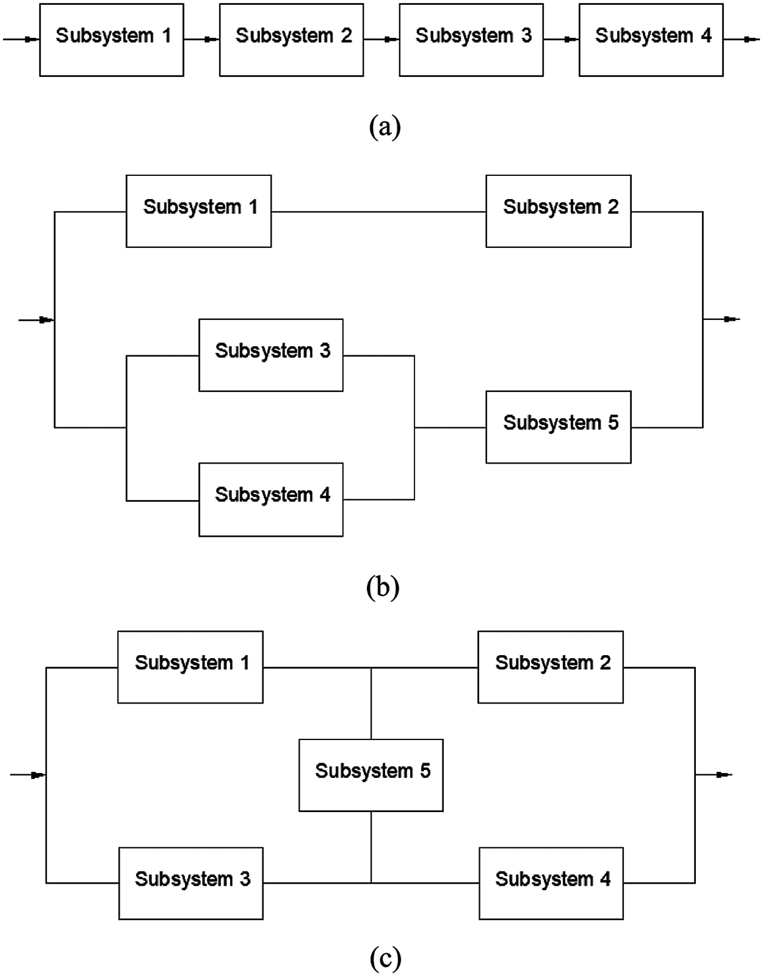
Figure 1: Representation of (a) series system; (b) series–parallel system; and (c) complex (bridge) system
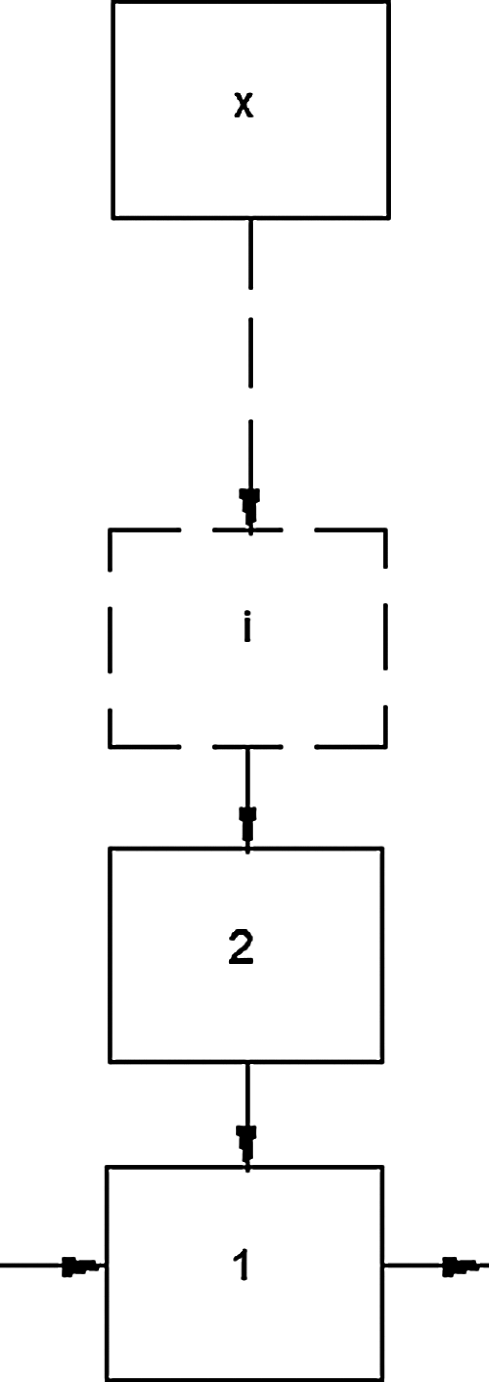
Figure 2: Representation of subsystem
For the reliability allocation problem, the system structure is fixed and the component reliability values are continuous decision variables. Component parameters (cost, weight, volume) are functions of the component reliability. Increasing the system reliability by using more reliable components rises the cost, and probably weight and volume, which may be incorporated as part of the constraints or the objective function.
The reliability-redundancy allocation problem is the most general problem formulation. Each subsystem has ni components with reliability of ri as decision variables. The challenge then is to assign redundancy and reliability optimally to the components of each subsystem in order to optimize the overall reliability of the system. The system and subsystems can be in any arrangement.
For each series, series–parallel, and bridge system, the reliabilities are defined, respectively, as:
where Ri is the reliability of the ith parallel subsystem, as defined by:
where xi is the redundancy allocation of the ith subsystem and ri is the individual component reliability of this subsystem. In all the following configurations, we consider xi as a discrete integer that ranges from 1 to 10 and ri as a real number that ranges from 0.5 to 1 × 10⁻⁶.
The aim of the RRAP is to improve the reliability of the entire system under a specified controlled environment, based on the cost, weight, and volume of the system. The system cost function
where n is the number of subsystems, and αi and βi are the parameters of the cost function of subsystems. The value 1000 in the equation is supposed to be the mean time between failures (i.e., the operating time during which the component must not fail).
Fig. 3 shows the evolution of the cost function of the reliability, in the cases of having 1 and 10 redundant components for one subsystem. The associated cost exponentially increases with reliability and the number of redundancy allocations. Fig. 4 shows the evolution of the cost function of redundancy allocation for two levels of reliability (i.e., 0.9 and 0.99), where the cost ration is 33.94 (for β = 1.5).
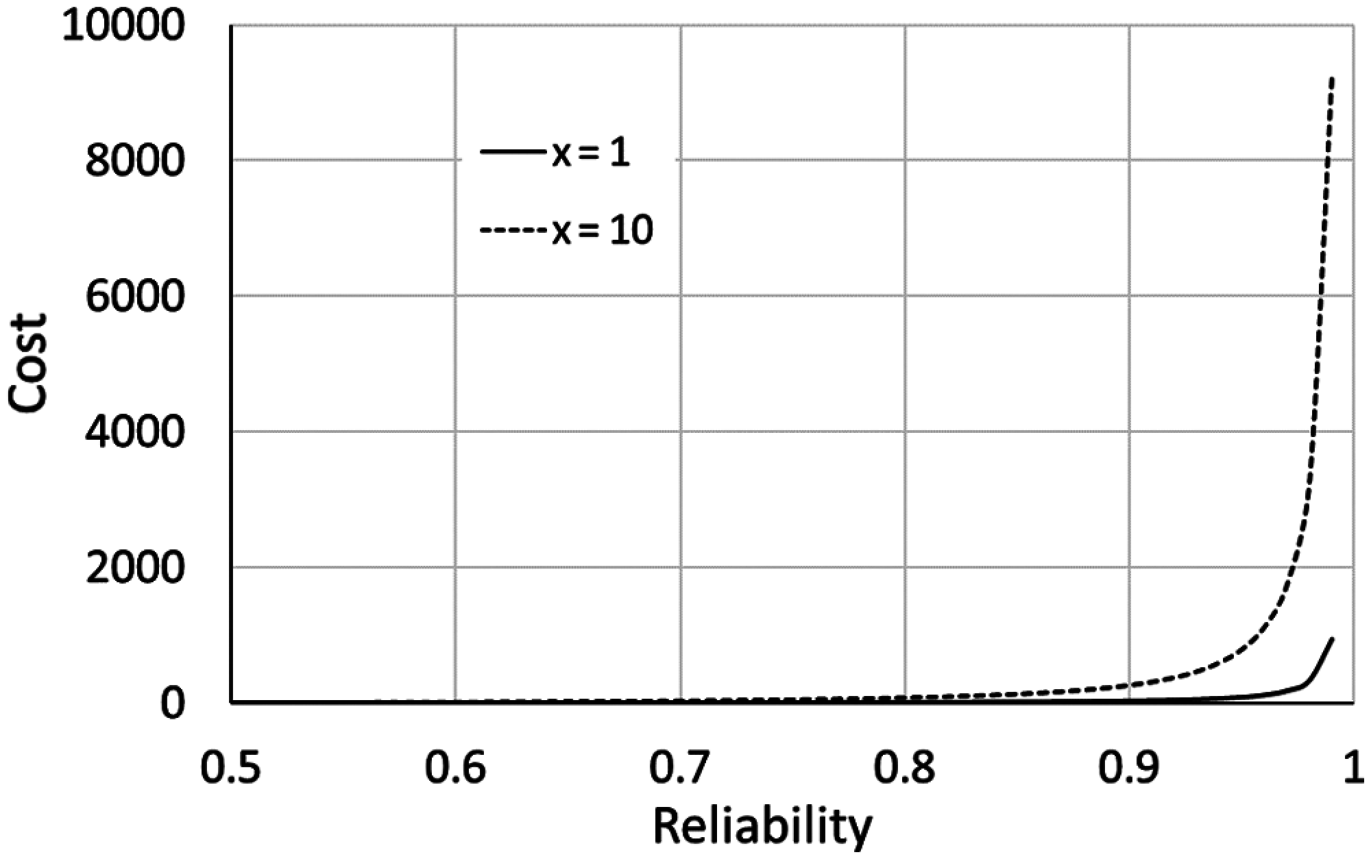
Figure 3: Evolution of the cost function of reliability (α = 2.3 × 10⁻⁵ and β = 1.5)
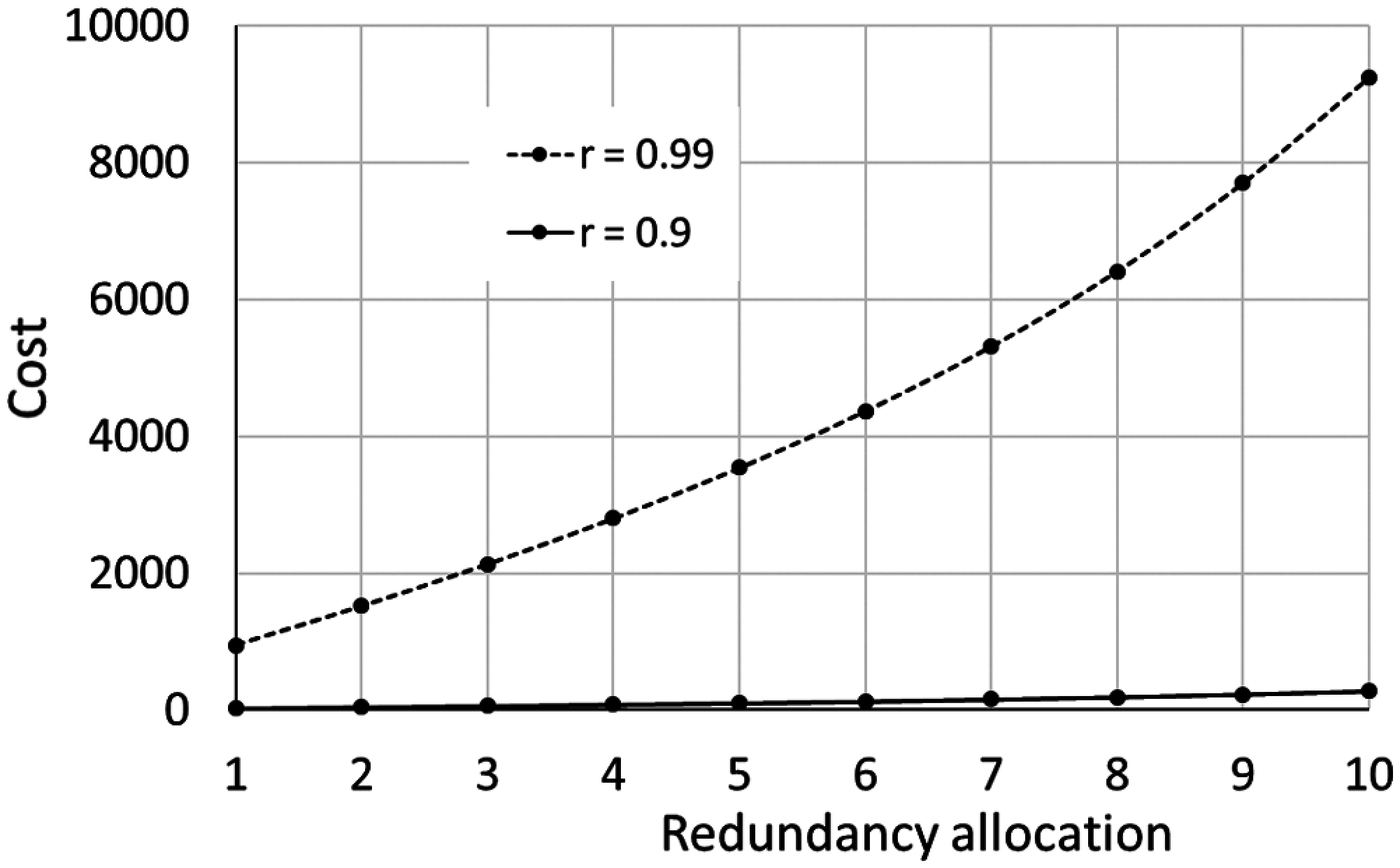
Figure 4: Evolution of the cost function of redundancy allocation (α = 2.3 × 10⁻⁵ and β = 1.5)
The weight function of the system depends on the number of components per subsystem and the number of subsystems, and can be defined as [30]:
where wi is the weight function parameter.
Early studies used a range of 3 to 9 for the weight function parameter [14,31–33]. The weight is found to increase exponentially with the reliability and the amount of redundancy allocation (Fig. 5).
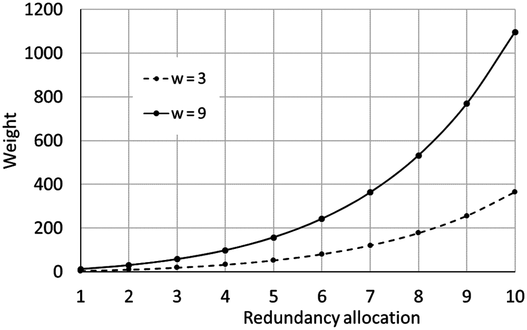
Figure 5: Evolution of the weight function of redundancy allocation
The system volume function also depends on the number of components per subsystem and the number of subsystems, and it can be defined as [30]:
where vi is the volume function parameter.
Fig. 6 shows the evolution of the subsystem volume function of redundant components.
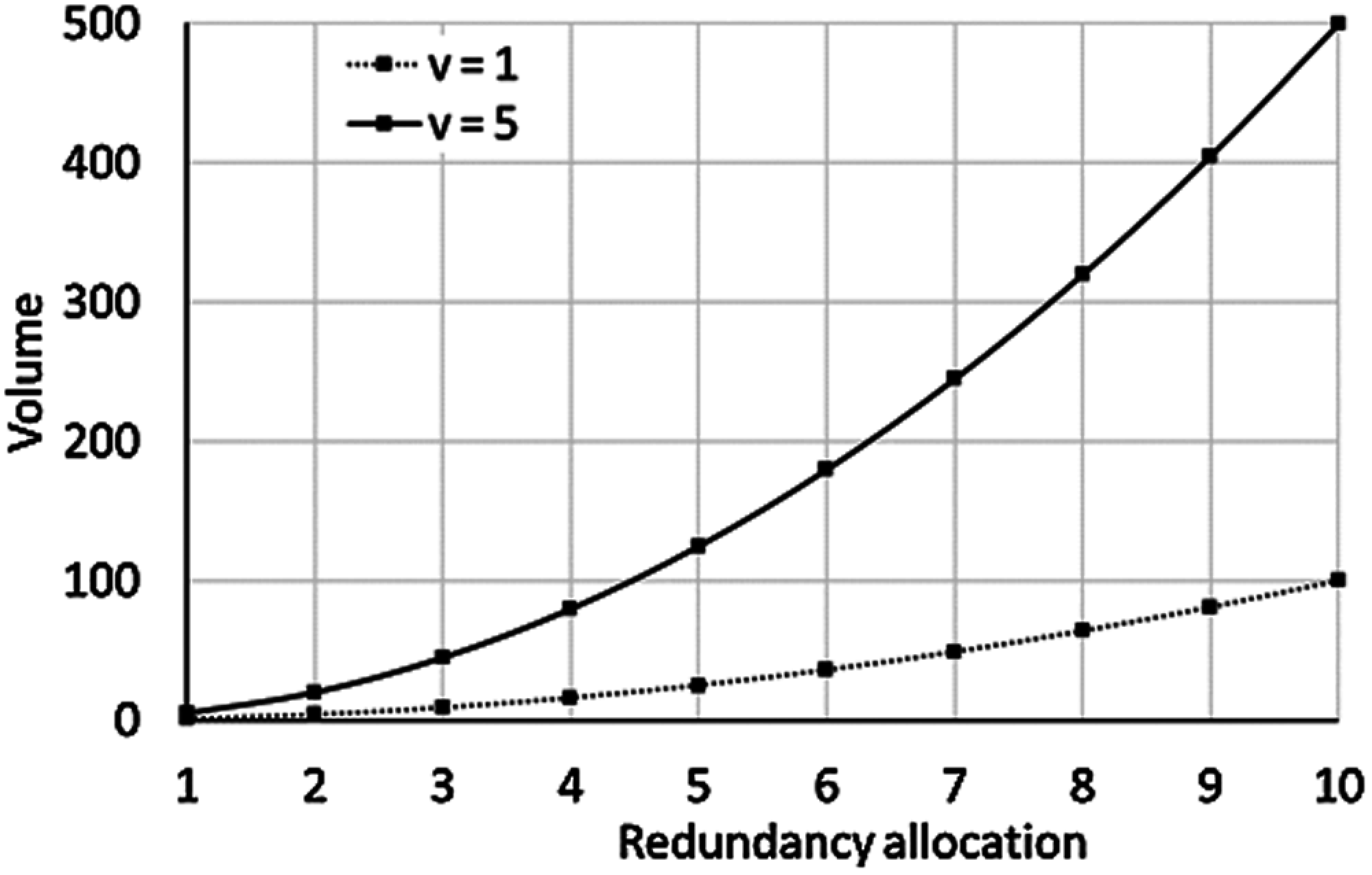
Figure 6: Evolution of the volume function of redundancy allocation (w = 3)
In summary, the general RRAP can be expressed in the following formulation, in which the reliability is considered as the objective function:
where C, W, and V are the upper bounds of the cost, weight, and volume of the system, respectively.
4 Evolutionary Algorithms Used for RRAP
All EAs share three common features: population, fitness, and evolution. Population represents the set of individual solutions that are initially randomized and then optimized to attain a final solution. A constant population size is generally maintained during the evolution process. Fitness ranks the population/solution according to some established performance criteria. Fitter individuals impact the remaining individuals through the evolutionary process. To explore a problem's solution space to attain the best population, random or controlled variation is important.
The first use of an EA for a system reliability problem was in the field of GA [34–36]. This work demonstrated that GAs are efficient, robust, cost-effective, and capable of finding the optimum in a high-dimensional nonlinear space [35]. evaluated the robustness of a GA and found that the optimum for a high-dimensional nonlinear space was identified in a significantly shorter time than required by enumeration. To improve the reliability of a personal computer, the authors defined the key components and their modes of failure to assess potential levels of improvement [36]. used GAs to improve the design, operation, and safety of new and/or existing nuclear power plants (subject to an overall plant safety objective) by optimizing the reliability allocation and minimizing total operating costs. In conjunction with a set of top-level performance targets, these authors determined the reliability characteristics of reactor systems, subsystems, main components, and plant procedures. Also, this GA had a multi-objective problem formulation that included the cost for enhancing and/or deteriorating a system's reliability into the reliability allocation process. GA has been shown to find successful solutions for a traditional pressurized water reactor that included multi-objective reliability optimization [37–41].
SA was first introduced by [42] and subsequently used in RRAP by [43]. Reference [43] proposed an SA algorithm for optimizing the reliability of the communication network. This SA selects an optimal set of links that optimize the overall reliability of the network. This is subject to cost constraints and permissible incidences of node links, connection costs, and connection reliability. SA has also been used to identify the best solution to system stability problems with redundancy allocation [44], which considers nonlinear resource constraints [45]. Additionally, various SA techniques have been applied to solve multi-objective system reliability optimization problems [46].
Reference [47] introduced PSO for optimization of continuous unconstrained functions. Initially, PSO did not attract much interest from the reliability community since most issues with reliability optimization are distinct and have constraints. However, properly adopted PSOs have been shown to be effective tools for solving some discrete problems of restricted reliability optimization [48,49]. applied PSO to solve reliability optimization for complex RAP systems.
Reference [50] introduced BCO. Later, [51,52] used BCO for application to RRAP [53]. introduced BBO for RRAP application. Later, BBO was also applied to RRAP by [32,54], and [55,56]. and [57] introduced AISO. Later, [58] applied AISO to an RRAP [59]. introduced the ICA [60–62] applied ICA to RRAP.
Timeline of the cited evolutionary algorithms is shown in Fig. 7.
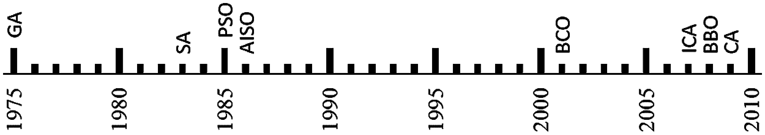
Figure 7: Timeline of the main evolutionary algorithms used for RRAP
The following algorithm descriptions are applied for RRAPs with these assumptions:
(1) The component supply is infinite, and all redundant components are similar for each individual subsystem.
(2) The failures of individual components are independent. Failed components do not harm the system and are not fixed.
(3) The weight, cost, and volume of the components are known and deterministic.
GA is based on genetic mechanism and the evolution of species by Darwin using concepts such as mutation, crossing over, the survival of the best individual, and natural selection [6,63,64]. Each individual of a population has two characteristics: a chromosome and a fitness value representing its quality. A chromosome is represented as a sorted string or vector. Chromosome representation is an essential task in GA, and a chromosome can be represented by different forms. In this paper, each chromosome/solution has 2n number of genes with the first n genes corresponding to the first n integer variables (redundant components) and the second n genes corresponding to floating point variables (reliability of components).
The evolutionary process begins when all fitness values of the initial population have been assigned. Each individual is evaluated on the basis of the results from the fitness function. The individual follows a selection process where the best (fittest) survives and is selected to continue regeneration and the others disappear. Parents exchange their genetic information randomly to produce an innovative child population. This process includes the selection of crossover and mutation operators. To maintain constant population size, parents are then replaced by children in the population. This reproduction (selection, crossover, and mutation) is repeated and takes place on the basis of the probability of crossover (Pc) and the probability of mutation (Pm). The procedure is iteratively subjected to an assessment of the solution's relevance until the solution reaches the global optimum with a defined iteration number.
The selection operator plays an essential role because it is the first operator applied to the population. The goal of this operator is to select above average solutions and to remove below average solutions from the population of the next generation using the Principle “survival of the relatively fit.” In this review, we define a size two tournament selection processes with replacement as the selection operator [65]:
• When both the chromosomes are feasible, the one with the higher fitness value is chosen.
• When one chromosome is feasible and the other is infeasible, the one that is feasible is chosen.
• When both chromosomes are infeasible with unequal constraint violations, the chromosome with the less constraint violation is chosen.
• When both the chromosomes are infeasible with equal constraint violations, then either chromosome is chosen.
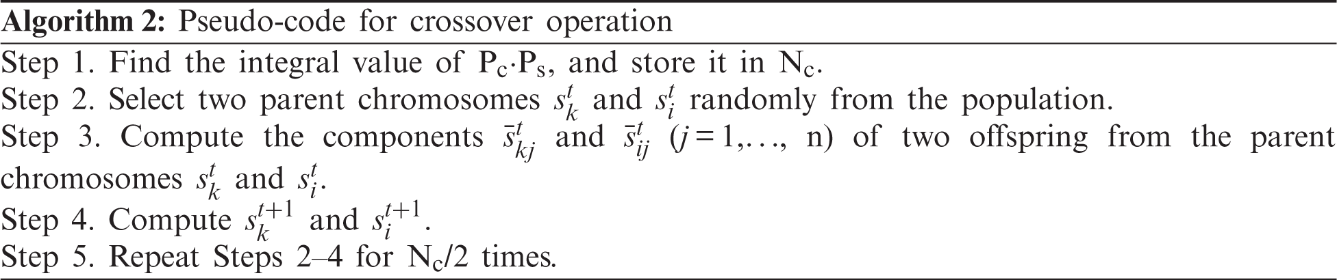
A crossover operator is added to the surviving chromosomes after the selection process. This is the operation that really empowers a GA. It simultaneously acts on two or more parent chromosomes and produces offspring by recombining features of the parent solutions. In this review, we describe an intermediate crossover for integer variables and a power crossover for floating point variables [65]. Crossover processes begin by defining the crossover population size (Pc⋅Ps). Then, two parent chromosomes
In the case of intermediate crossover,
where g is a random integer between 0 and.
In the case of power crossover,
where λ is a random number from a uniform distribution with the interval [0,1].
Finally, the new two children
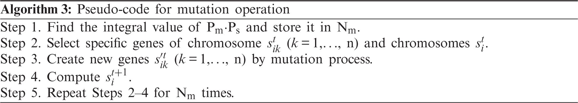
The purpose of the mutation procedure is to introduce random variations into the population. These random variations are used to prevent the search process from converging to local optima. The mutation process sometimes helps recover the data lost in previous generations and is responsible for the system's fine tuning. This operator only applies to a single chromosome. Usually, its rate is very low. In this review, we discuss the one-neighborhood mutation for integer variables method [66] and non-uniform mutation for floating point variables [65]. The mutation process starts by defining the mutation population size (Pm⋅Ps). Then, particular genes of chromosome
In the case of one-neighborhood mutation,
where ρ is a uniformly distributed random number in [0,1].
In the case of non-uniform mutation,
where ρ1 and ρ2 are two uniformly distributed random numbers in [0,1]. Mg is the maximum number of generations.
Thus, the final gene is
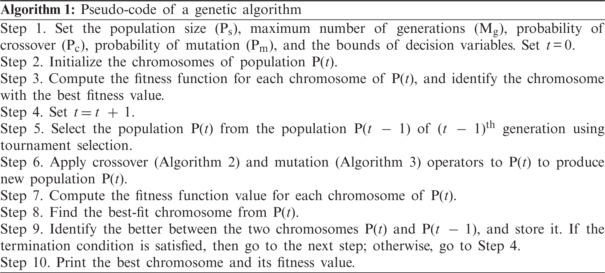
The different steps of a GA are summarized in the following pseudo-codes (Algorithms 1–3):
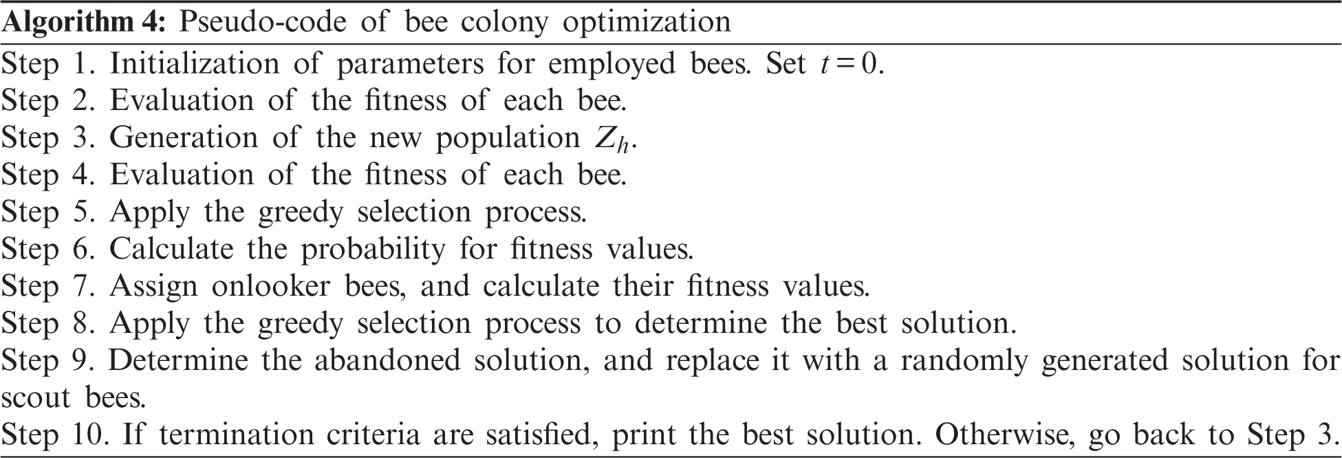
Developed by [50,67], the BCO algorithm mimics honey bee behavior. Bees in a colony are divided into three groups: employed bees (forager bees), onlooker bees (observer bees), and scouts. There is only one employed bee associated with each food source. An employed bee of a discarded food site is forced to become a scout who randomly searches for a new food source. Employed bees share information with onlooker bees in a hive so that onlooker bees can choose a food source for the forager.
In the initialization stage of a BCO, bees randomly select food source positions and nectar amounts are determined by a fitness function. These bees return to the hive and share this nectar source information with bees waiting in the dance area of the hive. Next, the second stage occurs, where every employed bee goes back to the same food source area visited during the previous cycle. Thus, the probability ph of an onlooker bee choosing a preferred food source at Xh is defined as
Here, N is the number of food sources and fh = f(Xh) is the amount of nectar evaluated by the employed bee. If a food source is tried/foraged without improvement for a specified number of explorations, then it is abandoned and the bee at this location will randomly move to explore new locations.
After a solution is generated, this solution is improved by using a local search by a process called the “greedy selection process” carried out by onlooker and employed bees. The greedy selection process is defined by the following equation:
where k ∈ {1, 2,…, N} and j ∈ {1, 2,…, D} are randomly chosen indices and D is the number of solution parameters. Although k is determined randomly, it has to be different from h. ϕ is a random number between [−1, 1] and Zh is the solution in the neighborhood of Xh = (Xh1, Xh2, …, XhD). With the exception of the selected parameter j, all other parametric values of Zh are the same as those for Xh (i.e.,
If a particular food source solution does not improve for a predetermined number of iterations, then a new food source will be searched for by its associated bee, who now becomes a scout. Then, this randomly generated food source is similarly allocated to this scout and its status is changed to scout for hire. Hence, another algorithm iteration/cycle begins until either the termination condition, maximum number of cycles, or relative error limit is reached.
The different steps of a BCO are summarized in the following pseudo-code:
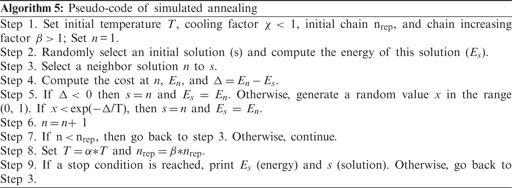
SA [42,68,69] is an approach to look for the global optimal solution (i.e., the lowest point in an energy landscape) by avoiding entrapment in poor local optima. This is accomplished by allowing an occasional uphill move to inferior solutions. The technique was developed on the basis of observations of how a normal crystalline structure arises from slowly cooled molten metal. A distinctive characteristic of this algorithm is that it combines random leaps into possible new solutions. This ability is controlled and reduced as the algorithm progresses.
SA emulates the physical concepts of temperature and energy. The objective function of an SA is treated as the energy of a dynamic system while the temperature is subjected to a randomized search for a solution. For a simulation, the state of the dynamic system is connected to the state of the system that is being optimized. The procedure is the following: The system is submitted to a high temperature and is then cooled slowly through a sequence of changes in temperature degrees. At each step, the algorithm searches for the state of system equilibrium using a series of elementary changes that are accepted if the energy system decreases. Smaller energy increments can be tolerated as the temperature decreases, and the device gradually falls into a low energy state. This property allows the algorithm to escape and close if the conditions are not similar to the global minimum from a local optimal configuration. The likelihood of acceptance and uphill movement depends on the temperature and the extent of the rise (Δ).
The algorithm begins by randomly choosing an initial solution (s) and then calculates the energy (Es) for s. After setting an initial temperature T, a neighbor finding strategy is used to produce a neighbor solution n to the current solution s and to determine the corresponding energy En. In the neighbor solution n, if the energy En is lower than the current energy Es, then the neighbor solution is set as the current solution. Otherwise, a probability function is evaluated to decide if the neighbor's solution can be recognized as the current solution. After thermal equilibrium is reached at the current temperature T, the value of T is reduced by a cooling factor χ and the number of internal repetitions is increased by an increasing factor β. The algorithm starts from the current solution point to pursue thermal equilibrium at the new temperature. The entire process stops when either the lowest energy point is found or no upward/downward jumps have been taken for a specified number of consecutive thermal equilibriums.
The SA algorithm requires several decisions to be made. These decisions concern the choice of energy function, cooling schedule, neighborhood structure, and parameters for annealing (i.e., initial temperature, cooling factor, increasing repetition factor of the inner loop, and stopping condition). Each decision must be made carefully because it affects the speed of the algorithm and the consistency of the solutions.
The key to success for the SA algorithm is the energy function. It forms the energy landscape and influences how a solution is found by the algorithm. The energy function reflects the objective function to be optimized for an allocation problem. The neighborhood determines the process to switch from a solution point to another solution point.
The cooling schedule describes the temperature reduction mechanism when an equilibrium state is reached. The number of inner loop repetitions (nrep) and the cooling rate (χ) control this process [70]. discussed a geometric cooling schedule, where the temperature (T) is lowered so that T = α ∗ T, where α is a constant less than 1. The chain (i.e., the number of repetitions of the inner loop) is modified at each temperature similarly: nrep = β ∗ nrep, where β is a constant greater than 1.
The annealing parameters are associated with the choice of initial temperature T, cooling factor α, increasing factor β, and stopping condition. These parameters are defined as follows:
• Initial temperature T: One of the most critical parameters in the SA algorithm representing the initial temperature. If the initial temperature is very high, the algorithm's execution duration becomes very long. By contrast, low initial temperature results in weak results. The initial temperature must be hot enough to allow neighboring solutions to be freely shared. A solution to this problem is to quickly heat the device until the ratio of accepted movements to rejected movements exceeds the necessary value. The ratio of approved movements to rejected movements (which reflects a volatile suitability scheme) can be determined in advance. The cooling schedule starts at this stage. A physical analogy of this technique is when a material is rapidly heated to its liquid state before slowly cooling according to an annealing plan.
Let T be the initial temperature; cr and ci be numbers corresponding to cost reduction and cost increase, respectively; ca be the average cost increase value of the ci trials; and a0 be the desired initial acceptance value. Then, the following relation may be represented by
which can be rearranged to give the initial temperature as
• Cooling factor χ: The cooling factor χ represents the rate at which the temperature T is decreased. For the success of any annealing operation, this aspect is crucial. A fast decrease yields a poor local optimum and causes a slow cooling time. Most of the literature report values between 0.8 and 0.95, with a bias toward the higher end of the range.
• Increasing factor β: The increasing factor β (>1) is the rate at which the internal number of repetitions increases as the temperature decreases. It is necessary to spend a long time at a lower temperature to assure that a local optimum has been thoroughly explored. The lower the temperature, the greater the number of repetitions of the inner loop.
• Stopping condition: The stop condition is expressed in terms of either the temperature parameter or the steady state of the system with the current solution. Other approaches describe a stopping state by designating several iterations or temperature thresholds that must have pass without approval. The simplest rule is to specify a total number of iterations and then stop when this number has been completed. In this paper, the final temperature is chosen to give a low acceptance value.
The different steps of SA are summarized in the following pseudo-code:
PSO was initially proposed and designed by [47]. It is inspired by the social behavior of bird flocking or fish schooling. The PSO algorithm works by randomly initializing a flock over a searching space, where each bird is called a “particle.” These “particles” fly at a certain velocity and find the global best position after iteration. At each iteration, each particle can adjust its velocity vector on the basis of its momentum, the influence of its best position (pbest), and the best position of its neighbors (gbest). Next, a new position is computed that the “particle” flies to. Suppose the dimension of the searching space is D, and the total number of particles is N, then the -position of the ith particle can be expressed by a vector xi = [xi1, xi2, …, xiD], the best position of the ith particle by the vector pbesti = [pbesti1, pbesti2, …, pbestiD], and the best position of the total particle swarm by the vector gbest = [gbest1, gbest2, …, gbestD]. If the velocity of the ith particle is represented by the vector vi = [vi1, vi2, …, viD], then its position and velocity at the (t + 1) iteration are updated using the following equations [29]:
where c1 and c2 are constants, ud and Ud are random variables with a uniform distribution between 0 and 1, w is inertia weight (representing the effect of the previous velocity vector on the new vector).
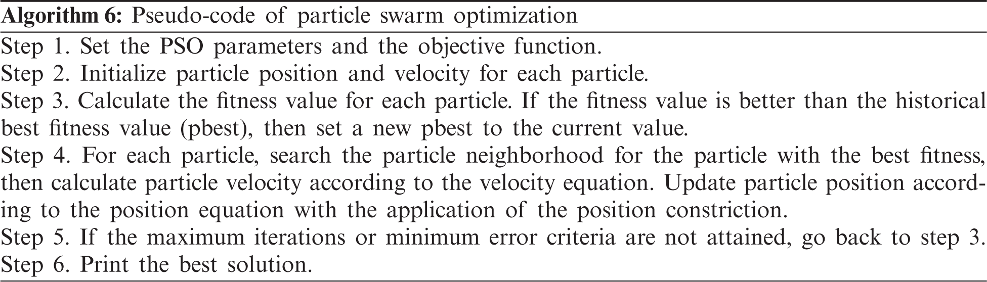
The different steps of PSO are summarized in the following pseudo-code:
Based on the concept of biogeography, BBO mimics the distribution of species that depend on rainfall, diversity of topographic features, temperature, land area, etc [32,53–55]. Biogeography describes how species migrate from one habitat to another, the creation of new species, and the extinction of species. A habitat is an island that is geographically isolated from other habitats. Each habitat is defined by a high habitat suitability index (HSI), which describes how geographically well suited it is for species living. Species have to emigrate or immigrate. If the high HSI habitats have more species, these species have more opportunities to emigrate to a neighboring habitat. For immigration, a species moves toward a high-HSI habitat that has fewer species.
The migration (i.e., immigration or emigration) of species in a single habitat is explained in Fig. 8. When there are no species in a single habitat, then the immigration rate λ of the habitat will be maximized (I). Conversely, when the number of species increases, then only a few species can successfully survive. Thus, the immigration rate is decreased and becomes zero when the maximum species count (Smax) is reached. The emigration rate (μ) increases with the increasing number of species. Hence, the emigration rate is higher for a more crowded habitat than a less populated habitat.
The first stage of the BBO algorithm is to assign the parameter values. These parameters are maximum species count (Smax), maximum migration rate (E), immigration rate (I), the maximum mutation rate (mmax), habitat modification probability (pmod), number of habitats, and number of iterations.
In the BBO algorithm, each individual or decision variable is considered to be a “habitat.” An HSI represents the measurement of an individual, and the length of the habitat depends on the number of decision variables. This HSI is a measure of the goodness of fit of the solution and is equivalent to the fitness value in population-based optimization algorithms. The corresponding variables of individuals that characterize the habitability feature are called suitability index variables (SIVs). These are randomly initialized within the maximum and minimum limits by
where Ud is a uniformly distributed random number between (0, 1). Each habitat in a population of size NP is represented by N-dimensional vector H = [SIV1, SIV2, …SIVN], where N is the number of SIVs (i.e., features) to be evolved to achieve an optimal HSI. HSI is the degree of acceptability calculated by evaluating the objective function (i.e., HSI = f(H)).
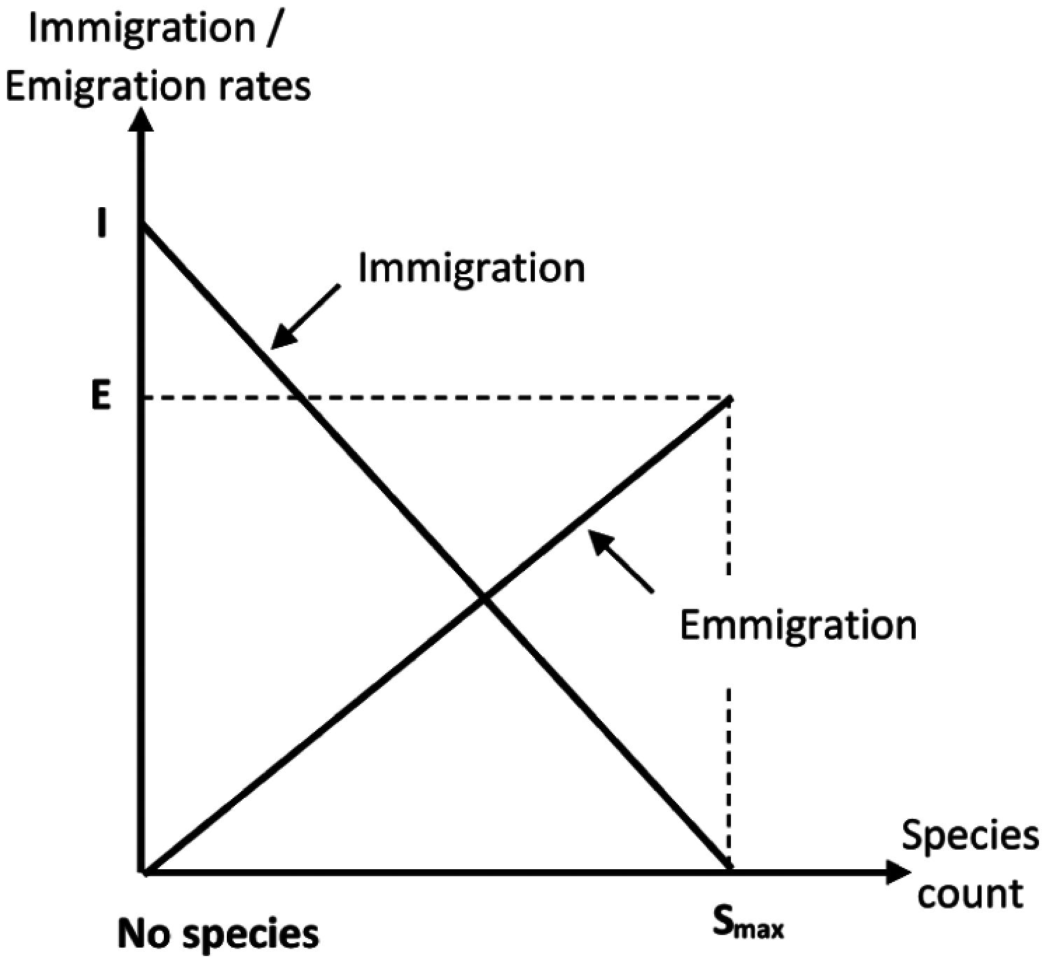
Figure 8: Evolution of immigration and immigration
Migration is an adaptive process that is used to change an existing habitat's SIV. Each individual has its own immigration rate (λ) and emigration rate (μ) to improve the solution and thus evolve a solution to the optimization problem. This solution is modified on the basis of its probability (Pmod), which is a user-defined parameter. Based on this probability, the immigration rate (λ) of each habitat is used to decide whether or not to modify each SIV. Then, another habitat is selected on the basis of emigration rate (μ). This habitat's SIV will randomly migrate to the previous habitat's SIV. A good solution is a habitat with a relatively high μ and low λ, whereas the converse is true for a poor solution.
High-HSI habitats resist change more than low-HSI habitats. Weak solutions consider more helpful knowledge from successful solutions that increase the algorithm's ability to exploit. The immigration and emigration rates are initially based on the number of species in the habitat and are calculated by
where I is the maximum possible immigration rate, E is the maximum possible emigration rate, k is the number of species for the kth individual, and Smax is the maximum number of species. I and E are often set equal to1 or slightly less than 1.
Besides migration, BBO includes a mutation feature. Mutation is used to improve population diversity to obtain the best solution. Low- and high-HIS-valued habitats have less possibility to mutate than average-HIS-valued habitats. For instance, let us assume that there are a total of Smax habitats and there are S Species in the Sth habitat. For the Sth island, the immigration rate is λs and the emigration rate is μs. By considering PS as the probability that there are exactly S species living in a habitat, PS changes from time t to t + Δt by
By taking the limit of the previous equation:
where PS−1, PS, and PS+1 are the species count probabilities; λS − 1, λS, and λS + 1 are immigration rates; and μS − 1, μS, and μS + 1 are emigration rates of the habitat for S − 1, S, and S + 1 species, respectively. Smax is the maximum species count in the habitat. The steady state probability of the quantity of each species is as follows:
Thus, on the basis of the randomly selected SIV habitat modified based on mutation rate m and for the case of E = I, m is calculated as
where mmax ∈ [0,1] is the predefined parameter called the maximum mutation probability, pmax = max (P1, P2, …, PNP), where NP is the number of habitats and Pi is the probability of habitat i, which can be calculated using Eq. (6). The goal of this mutation scheme is to increase population diversity, thus, minimizing the risk of the solution being stuck in local optima.
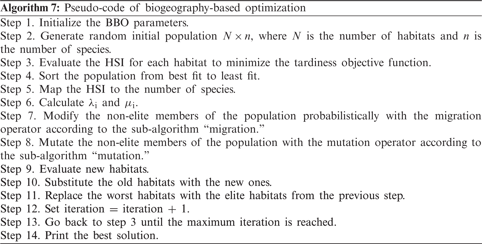
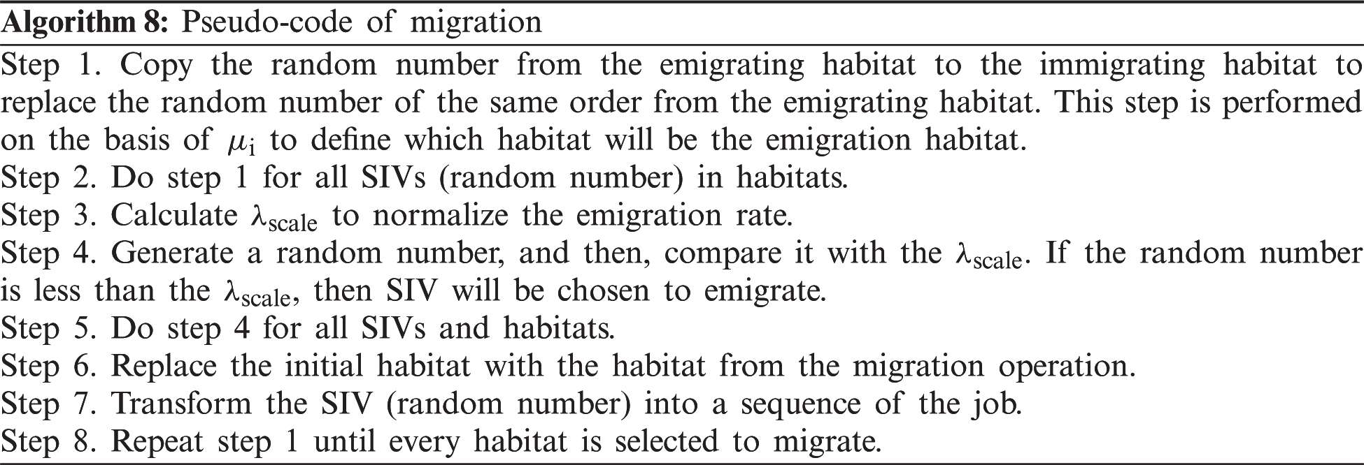
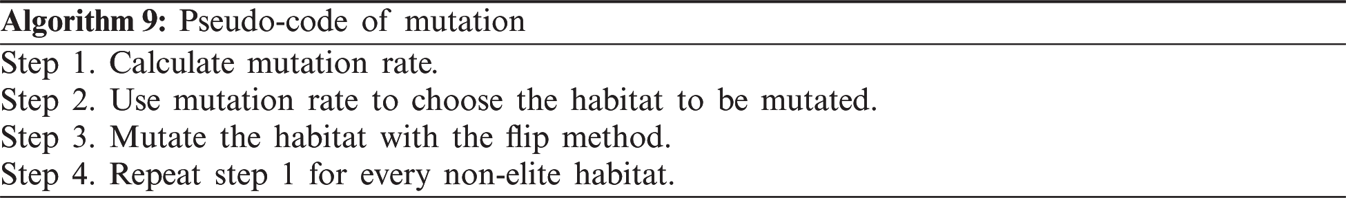
The different steps of BOO are summarized in the following pseudo-codes (Algorithms 7–9).
AISO was first introduced by Rechenberg [71]. The natural immune system is a very complex mechanism of protection against pathogenic species. The immune system is divided into a two-tier line of defense: the innate immune system and the adaptive immune system. The fundamental components are lymphocytes and antibodies [56,72]. The cells of the innate immune system are readily available to defend against a wide range of antigens without prior exposure. In response to a particular infectious agent (antigen), the generation of antibodies is a lymphocyte-mediated adaptive immune response responsible for the identification and removal of pathogenic agents [73]. The cells in the adaptive system can establish an immune memory so that when exposed again, the system will identify the same antigenic stimulus. Additionally, all antibodies are only developed in response to particular infections. B-cells (B-lymphocytes) and C-cells (T-lymphocytes) are two major types of lymphocytes. They carry surface receptor molecules that can recognize antigens. The B-cells produced by the bone marrow display a distinct chemical structure and can be programmed to produce only one antibody that acts as a receptor on the outer surface of the lymphocyte. The antigens only bind to these receptors, thus, making them a compatible match [74].
The immune system's main role is to recognize and remove intruders so that the immune system has the potential for self/non-self-discrimination. As previously discussed, different antibodies can be produced and specific antigens can be recognized. The antibody-recognized part of the antigen is called the epitope, which functions as an antigen determinant. Every type of antibody has its own specific antigen determinant, which is called an idiotope. Additionally, an activated lymphocyte needs to proliferate and then differentiate into effector cells to generate sufficient unique effector cells to counter an infection. This approach is called clonal selection [75] and is accompanied by genetic operations to form a large plasma cell clone. The antibodies can then be secreted and made ready for binding to antigens. On the basis of the above facts, [76] proposed an idiotope network hypothesis that is based on the clonal selection theory. In this hypothesis, some types of recognizing sets are activated by some antigens and create an antibody that activates other types of recognizing sets. Activation is propagated through antigen-antibody reactions throughout the entire network of recognition sets. It should be noted that detection of an antigen is not achieved by a single or multiple recognition sets but rather by interactions between an antigen and an antibody.
From this viewpoint, an antibody and an antigen can be viewed as the solution and objection function, respectively, to solve the problem of reliability–redundancy allocation optimization.
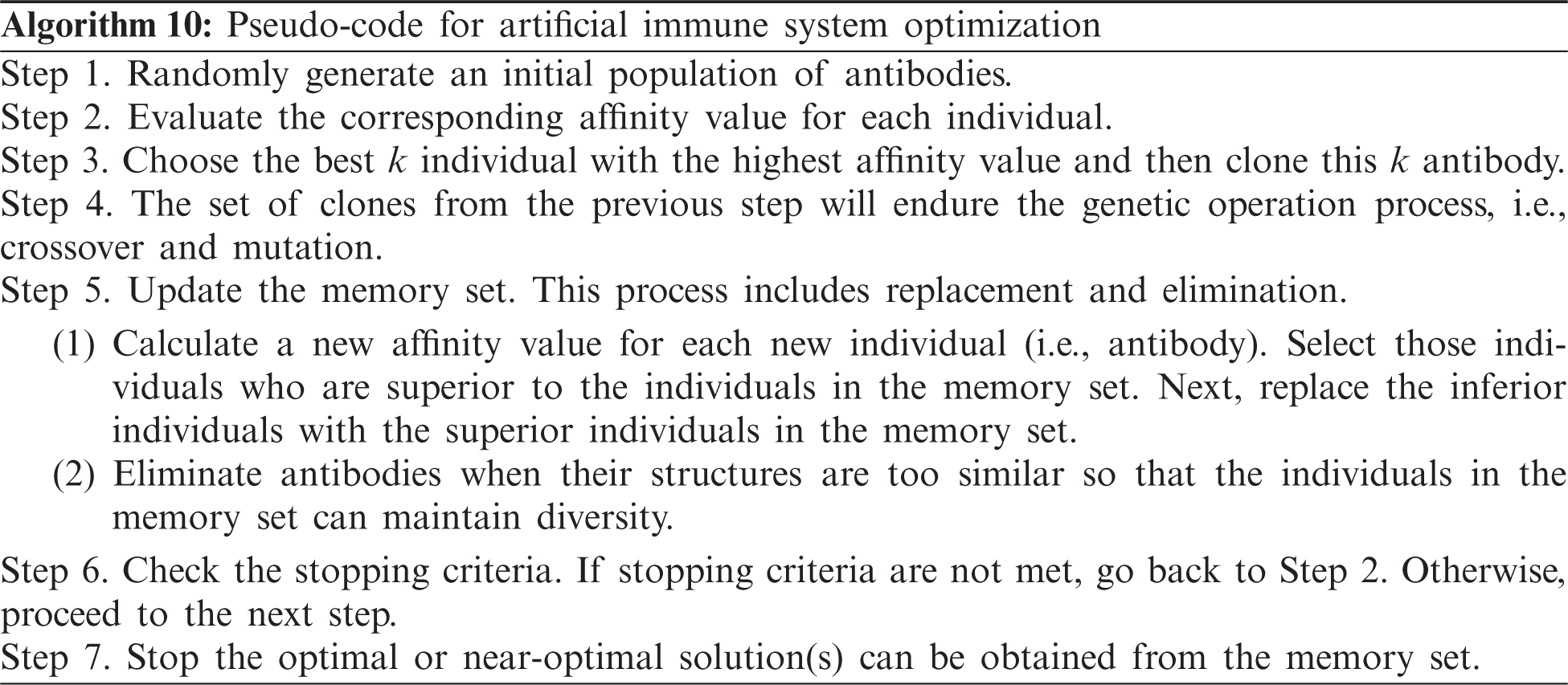
The different steps of an AIS are summarized in the following pseudo-code:
CS was introduced by [77]. It was inspired by the aggressive reproduction strategy of cuckoos. Cuckoos lay their eggs in the nests of other host birds, which may be of various species. The host bird may notice that the eggs do not belong, in which case, either the eggs are destroyed or the nest is abandoned altogether. This contributed to the creation of cuckoo eggs that resemble the eggs of local host birds. CS is based on three idealized rules:
• Each cuckoo lays one egg at a time and deposits it in a randomly picked nest.
• The best nests with high-quality eggs (i.e., solutions) will be passed on to the next generations.
• The number of available host nests is set, and an alien egg can be discovered by a host with a probability of pa ∈ [0,1]. In this scenario, the host bird may either throw the egg away or leave the nest to establish an entirely new nest in a new location.
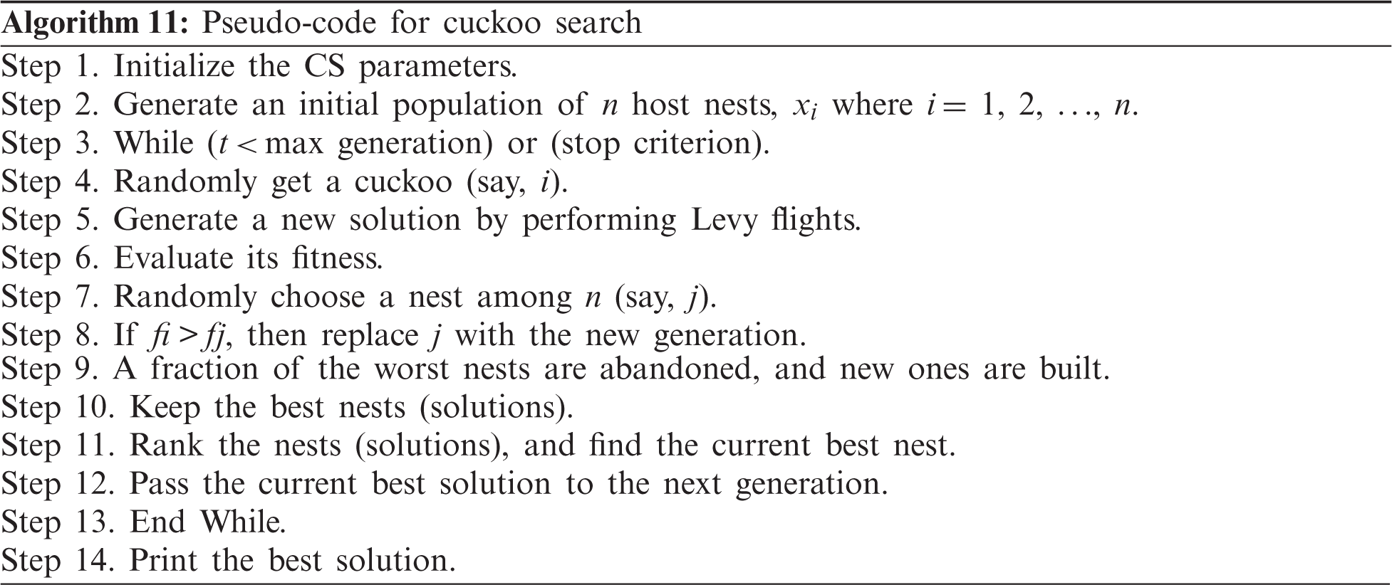
For simplicity, this last statement can be approximated by the fraction of nests that are replaced by new nests with new random solutions. As with other evolutionary methods, the solution's fitness function is described similarly. In this process, an egg already present in the nest will represent the previous solution, whereas the cuckoo's egg represents the new solution. The goal is to replace worse solutions that are in the nests with new and theoretically better solutions (cuckoos). The basic steps of a cuckoo search are defined in Algorithm 11 on the basis of these three rules.
The new solution xi(t + 1) of the cuckoo search is based on its current location xi(t) and its probability of transition with the following equation:
where α (α > 0) represents the step size. This step size should be related to the problem specification, and t is the current iteration number. The product
In Mantegna's algorithm, the step length is calculated by
where u and v are drawn from the normal distribution, i.e.,
where the distribution parameter α ∈ [0.3,1.99] and Γ denotes the gamma function.
The steps of a CS are summarized in the following pseudo-code:
The ICA was recently introduced by [59]. The imperialist competitive uses imperialism and the imperialistic competition process as its source of inspiration. ICA is based on the actions of imperialists attempting to conquer colonies. It attempts to mimic the sociopolitical evolution of humans. Similar to other population-based algorithms, ICA starts with a randomly generated population called “countries.” These countries are divided into imperialists and colonies. The imperialists are the best candidate solutions, and the colonies are the remaining solutions. All the colonies will be shared among the imperialists according to each imperialist's powers. The more powerful the imperialist, the more colonies it possesses. An imperialist with its colonies forms an empire. In an ICA, the main action that leads the search for better solutions is colony movement toward the imperialists. This mechanism makes the population converge to certain spots in the search space where the best solution found so far is located.
One characteristic of the imperialism policy is that over time, colonies start to change their culture to be more similar to their respective imperialist. In ICA, this process is implemented by moving the colonies toward their imperialist in the search space domain and is called assimilation. During this event, a colony may become more powerful than its imperialist. In this case, the colony takes the place of the imperialist and the imperialist becomes the colony.
Imperialistic competition is ruled by the fact that the most powerful empires tend to increase their power, whereas the poorest ones tend to collapse. This phenomenon makes the number of imperialistic countries decrease during the run of the algorithm and the colonies of the defeated imperialist become part of another empire.
These two mechanisms force the algorithm to converge into a single empire, in which the imperialist and the colonies will have the same culture. Translating the ICA's metaphor into optimization language, the culture is a possible solution and the power is used to measure a country's objective function evaluation.
ICA starts by the initialization process (i.e., initialization of the empires) and then the medialization of the movement of colonies toward the imperialist (i.e., assimilation), the evaluation of the total cost of the empire, and finally the realization of imperialist competition.
In ICA, the countries are the possible solutions in the search space. They are represented by a 1xNvar dimension array defined by
In the beginning, an initial population is randomly created from a uniform distribution and it is divided into imperialists and colonies. Since ICA is a maximization algorithm, the imperialists will be the countries with the highest costs. Since the proposed problems are maximization problems, the cost of a country is given by the inverse of the cost function f defined by
The colonies will be distributed among the imperialists concerning the power of each imperialist. For this purpose, the normalized cost is defined by
where cn is the cost of nth imperialist and Cn is its normalized cost.
Finally, the normalized power for each imperialist is defined by
where Nimp is the number of imperialists. The normalized power of an imperialist represents the number of initial colonies this imperialist possesses, and it is given by
where N⋅Cn is the initial number of colonies of the nth empire and Ncol is the number of colonies.
The assimilation process (i.e., movement of colonies toward the imperialist) depends on the distance between the colonies and their imperialist, a real constant called an “assimilation coefficient,” and a random number in the range [0,1]. The following equation represents the new position of a colony:
where Posi is the vector of a colony's position on the ith iteration, γ is the assimilation coefficient, δ is a random number normally distributed between [0,1], and d is an Nvar dimension vector containing the distance between the colony and its imperialist. In imperialistic terms, d represents how different the culture of a colony is from the imperialist culture.
After this movement, a colony may reach a position with a higher cost than the imperialist. In this case, the colony will become the new imperialist, whereas the old imperialist will become a colony of the same empire.
The cost of an empire is most affected by the imperialist cost, although it is also affected by the colonies’ costs. This event is stated by
where T⋅Cn is the total cost of the nth empire and ε is a positive constant that represents the significance of the colonies’ costs.
The imperialistic competition comprises disputes between empires to possess the colonies. This event increases the powers of the most powerful empires, whereas the poorest empires tend to decrease their powers. Imperialistic competition is proposed by choosing the poorest colony (the colony with the higher cost) from the poorest empire to be disputed by the other empires. For this purpose, it is assumed that
where T⋅Cn is the total cost of the nth empire and N⋅T⋅Cn is its normalized cost. The possession probability ppn for the nth empire is given by
This creates the vector P with the possession probability of each empire and the vector R (of the same size of P) with random numbers uniformly distributed between [0,1] defined as
The vector D is defined by
Finally, the empire chosen to possess the colony is the one that has the highest value of D.
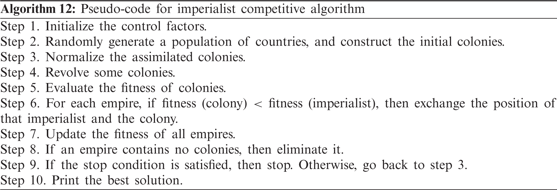
Different steps of ICA are summarized in the following pseudo-code:
5 Constraints Handling Techniques for Constrained Mixed Integer Nonlinear Problems
With the aid of an EA, several approaches have been suggested to deal with the constraints for solving restricted optimization problems. The penalty function method is a very common technique in RRAP. With this method, the restricted optimization problem is translated into an unrestricted one. Here, the reduced objective function contains the original objective function, and a penalty is imposed for breaching the constraints. Recently, a penalty function approach to handle the constraints has been proposed [78,79]. In this approach, when converting the constrained optimization problem into an unconstrained one, a large negative value (say, −M) is blindly assigned to the objective function for the infeasible solution for a maximization problem. In this case, if the constrained optimization problem is
then the reduced unconstrained optimization problem is as follows:
And
For a minimization problem, instead of −M, +M is used. In this work, we used the value of 99,999 for M.
Besides these “classical” problems, we consider a fourth benchmark problem for RRAP. This problem represents the overspeed protection system for a gas turbine (Fig. 9). Overspeed detection is continuously provided by electrical and mechanical systems. When overspeed occurs, it is necessary to cut off the fuel supply. For this purpose, four control valves Vi (i = 1, …, 4) must close. The control system is constructed as a four-stage series system. The goal of the optimization process is to determine an optimal level of ri and ni at each stage i with a maximum overall reliability system. The reliability is formulated as [72]:
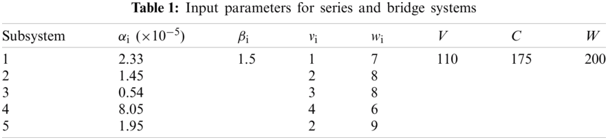
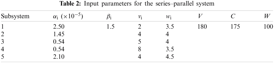
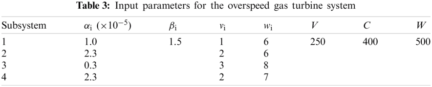
The values of the input parameters for series and bridge, series–parallel, and overspeed gas turbine system problems are provided in Tabs. 1–3, respectively (i.e., number of subsystems; component cost, volume, and weight values; and maximum value for the cost, volume, and weight), as stipulated in the literature.
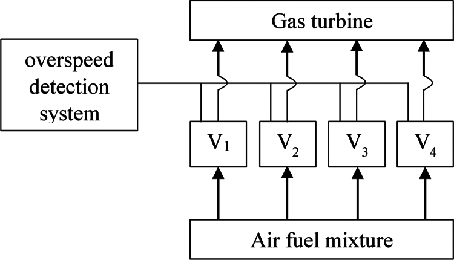
Figure 9: Overspeed gas turbine system
To compare the performance of each EA results, we define the maximum possible improvement (MPI) index [80] as follows:
where
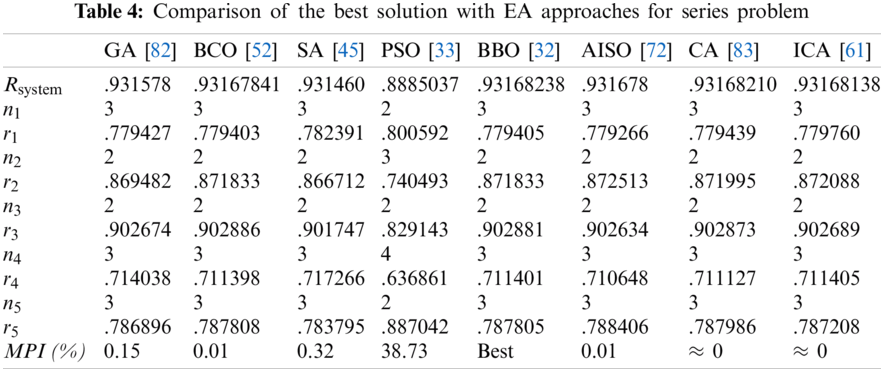
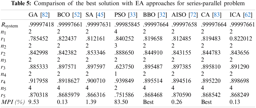
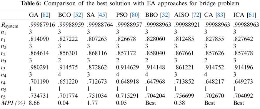
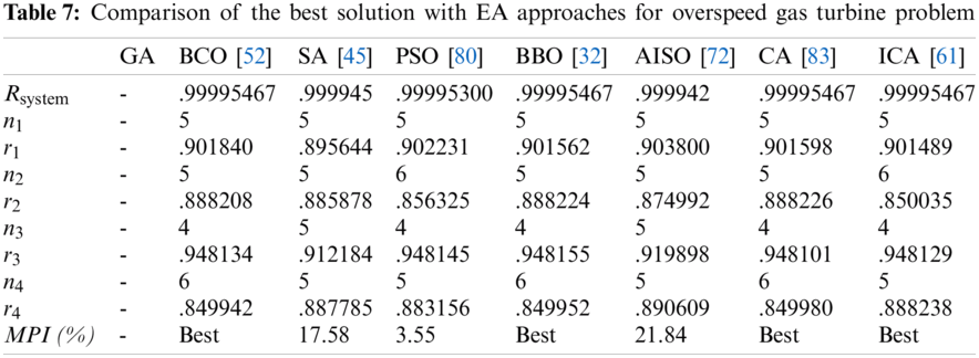
Tabs. 4–7 detail the best found solution of each EA for series, series–parallel, complex, and overspeed gas turbine system problems, respectively. The literature MPI values ranged from 1998 (GAs) to 2016 (ICAs). For the series problem, we note that for all of the EA (except PSO), the overall reliabilities were close (Rsys = 0.931xxx) with an MPI less than 0.32%. The best result was obtained by BBO and the worst by PSO. For the series–parallel problem, we also note that for all EAs (except PSO), the overall reliabilities were close (Rsys = 0.99997xxx) with an MPI range of 0.13%–9.53%. The best result was obtained by CA, and the worst, by PSO. For the bridge problem, all EA results were relatively small. The overall reliabilities were close (Rsys = 0.9998xxx). Except for GA (which has an MPI of 8.66%), the MPI range was 0.04%–1.77% for the other EAs. The best results were obtained by BBO, CA, and ICA, and the worst, by GA. For the gas turbine problem, the results from the literature ranged from 2006 to 2016. The results are considered to be disruptive. Indeed, the MPI range from 3.55% to 21.84%, corresponding to an overall reliability system close to 0.9999xxx. The best result was obtained by BCO, BBO, CA, and ICA, and the worst, by SA.
Generally, even if the improvement in the proposed approaches seems extremely small, small improvements in reliability are often hard to achieve in high-reliability applications. The best results are obtained by the latest developed approaches such as BBO (2015), CA (2016), and ICAA (2016). Recently, new approaches combine different EAs sequentially or in parallel. Tab. 8 shows the best found results using hybrid approaches. For series and gas turbine problems, CDEPSO [81] seems to be the best technique. CDEPSO combines PSO with differential evolution and chaotic local search. However, the results are the same as previously detailed in Tabs. 4 and 7. Hybrid techniques are more efficient with series–parallel and bridge problems. Indeed, combined GA-PSO [65] improves the overall reliability by 99% (i.e., MPI calculation).
7 Future Challenges in RRAP Optimization
Nowadays, the modern complex system reliability optimizations arise a certain challenges linked to ‘pragmatism’ by dealing with more realistic reliability behaviors of the components. Indeed, the previous problem formulations and assumptions are considering notions like the active redundancy, perfect switching of redundant components, binary behavior of components/systems,… which make the ideal problem far away from the realistic case.
For example, considering the ideal binary state (functioning/failed) for components and systems is not a realistic description of the multi-state system reliability behavior [84]. The first attempts to optimize such problems was presented by [48,85]. Substantial research efforts have been dedicated to the solution of RAP for series-parallel multi-state systems [48,86–89] over the last two decades. Parallel series structures are generally taken into account because they are very common in practice, but potentially mathematically cumbersome.
Moreover, with active redundancy assumption, the failure time of a parallel subsystem of components is the maximum of individual component failure times, and the reliability is defined by standard probability approaches [14]. Many real subsystem design issues, however, use a number of active, cold, warm or hot standby, sometimes within the same design, and thus the original formulations and methods of solution were not feasible or relevant to many real problems.
System designs with active redundancy have fully activated components that, in the event of a primary component failure, will continue to provide the requisite design functions until all redundant components have also failed. The use of non-activated components that can be turned on in response to a primary component failure includes cold standby redundancy. Cold standby redundancy includes failure detection switches and redundant unit activation. When active or cold-standby redundancies can be selectively selected for individual subsystems, researchers prefer to optimize reliability [90–95].

Another weakness of the idealization reliability assessment is the certainty approach considering the input parameter values. Intrinsic uncertainty and imperfect knowledge of system behavior, however, are still present. As aspects, factors and causes of uncertainty, we note lack of information and knowledge, model approximation, conflicting nature of information, measurement errors, … [14,96,97]. Uncertainty analysis defines the uncertainty in the model output that outcomes from uncertainty in the model inputs [98]. In the reliability engineering field, there is random and epistemic uncertainty [99,100]. Random phenomenon obeys to probabilistic modeling and Epistemic uncertainty consists in quantifying the degree of belief of the analysts on how well it represents the actual system. Recent researches are focusing on modelling and optimizing of multi-state systems under random and epistemic uncertainties [101–106].
System reliability optimization remains an ongoing topic of scientific improvement. New methods and algorithms are produced on the basis of mathematical advancements and new optimization approaches. This paper presented an overview of reliability–redundancy allocation problems with a focus on series, series–parallel, bridge, and overspeed gas turbine systems. EAs used for reliability–redundancy allocation problems were reviewed, along with their mathematical background and pseudo-codes detail. We reviewed EA on the basis of mimicry of social behavior of mankind and animals, biological interactions, and even the behavior of cooled molten metal (i.e., GAs, ant colony optimization, BCO, SA, PSO, BBO, Tabu Search, AISO, CA, and ICA).
RRAP optimization was investigated by GAs in 1995. The literature review presented in this paper summarized the best found results for each EA. All the cited techniques are promising and viable tools to solve RRAP. However, recent techniques such as the BBO (2015), CA (2016), and ICA (2016) generate the best results. Additionally, recent investigations tend to merge different techniques and sometimes generate better results than the use of a single algorithm.
Finally, we discussed current issues that require more complex systems with far more practical component/system reliability behaviors and that contain multi-state, uncertain data. Nevertheless, new perspectives are emerging, and effective approaches to addressing new challenges and more complex systems will need to be sought.
Funding Statement: The authors extend their appreciation to the Deanship of Scientific Research at King Saud University for funding this work through the Undergraduate Research Support Program.
Conflicts of Interest: The authors declare that they have no conflicts of interest to report regarding the present study.
1. V. M. Ordyntsev, “Some principles of design of a system for overall automation of large-scale chemical plant and the optimizing of this system,” IFAC Proceedings Volumes, vol. 1, no. 1, pp. 1829–1836, 1960. [Google Scholar]
2. B. Gluss, “An introduction to dynamic programming,” Journal of the Staple Inn Actuarial Society, vol. 16, no. 4, pp. 261–274, 1961. [Google Scholar]
3. R. Bellman, “The theory of dynamic programming,” Proceedings of the National Academy of Science of the United States of America, vol. 38, no. 8, pp. 716–719, 1952. [Google Scholar]
4. P. M. Ghare and R. E. Taylor, “Optimal redundancy for reliability in series systems,” Operations Research, vol. 17, no. 5, pp. 838–847, 1969. [Google Scholar]
5. G. B. Dantzig, A. Orden and P. Wolfe, “The generalized simplex method for minimizing a linear form under linear inequality restraints,” Pacific Journal of Mathematics, vol. 5, no. 2, pp. 183–195, 1955. [Google Scholar]
6. H. J. Bremermann, “Optimization through evolution and recombination,” Self-Organizing Systems, vol. 93, pp. 1–12, 1962. [Google Scholar]
7. G. B. Dantzig, “Reminiscences about the origins of linear programming,” Operations Research Letters, vol. 1, no. 2, pp. 43–48, 1982. [Google Scholar]
8. P. Wolfe, “Recent developments in nonlinear programming,” Advances in Computers, vol. 3, pp. 155–187, 1962. [Google Scholar]
9. R. E. Gomory, “Some polyhedra related to combinatorial problems,” Linear Algebra and its Applications, vol. 2, no. 4, pp. 451–558, 1969. [Google Scholar]
10. R. Bellman and S. Dreyfus, “Dynamic programming and the reliability of multicomponent devices,” Operations Research, vol. 6, no. 2, pp. 200–206, 1958. [Google Scholar]
11. R. E. Bellman and S. E. Dreyfus, “Applied dynamic programming,” Princeton, NJ, USA: Princeton University Press, 2015. [Google Scholar]
12. D. E. Fyffe, W. W. Hines and N. K. Lee, “System reliability allocation and a computational algorithm,” IEEE Transactions on Reliability, vol. R-17, no. 2, pp. 64–69, 1968. [Google Scholar]
13. Y. Nakagawa and S. Miyazaki, “Surrogate constraints algorithm for reliability optimization problems with two constraints,” IEEE Transactions on Reliability, vol. R-30, no. 2, pp. 175–180, 1981. [Google Scholar]
14. D. W. Coit and E. Zio, “The evolution of system reliability optimization,” Reliability Engineering & System Safety, vol. 192, pp. 106259, 2019. [Google Scholar]
15. D. W. Coit and J. C. Liu, “System reliability optimization with k-out-of-n subsystems,” International Journal of Reliability, Quality and Safety Engineering, vol. 7, no. 2, pp. 129–142, 2000. [Google Scholar]
16. K. B. Misra and U. Sharma, “An efficient algorithm to solve integer-programming problems arising in system-reliability design,” IEEE Transactions on Reliability, vol. 40, no. 1, pp. 81–91, 1991. [Google Scholar]
17. M. Gen, K. Ida, M. Sasaki and J. U. Lee, “Algorithms for solving large-scale 0–1 goal programming and its application to reliability optimization problem,” Computers & Industrial Engineering, vol. 17, no. 1–4, pp. 525–530, 1989. [Google Scholar]
18. R. B. Corotis and A. M. Nafday, “Application of mathematical programming to system reliability,” Structural Safety, vol. 7, no. 2–4, pp. 149–154, 1990. [Google Scholar]
19. D. Song, J. Liu, J. Yang, M. Su, S. Yang et al., “Multi-objective energy-cost design optimization for the variable-speed wind turbine at high-altitude sites,” Energy Conversion and Management, vol. 196, pp. 513–524, 2019. [Google Scholar]
20. A. Der Kiureghian and J. Song, “Multi-scale reliability analysis and updating of complex systems by use of linear programming,” Reliability Engineering & System Safety, vol. 93, no. 2, pp. 288–297, 2008. [Google Scholar]
21. J. E. Byun and J. Song, “Linear programming by delayed column generation for bounds on reliability of larger systems”, in 13th Int. Conf. on Applications of Statistics and Probability in Civil Engineering, Seoul, South Korea, 2019. [Google Scholar]
22. F. A. Tillman, C. L. Hwang and W. Kuo, “Determining component reliability and redundancy for optimum system reliability,” IEEE Trans. Reliab, vol. R-26, 1977. [Google Scholar]
23. F. A. Tillman, C. L. Hwang and W. Kuo, “Optimization techniques for system reliability with redundancy—A review,” IEEE Transactions on Reliability, vol. R-26, no. 3, pp. 148–155, 1977. [Google Scholar]
24. E. Pistikopoulos and C. A. Floudas, “Nonlinear and mixed-integer optimization. fundamentals and applications,” Journal of Global Optimization, vol. 12, pp. 108–110, 1998. [Google Scholar]
25. L. Qu, C. Han, Y. Li, K. Gao and R. Peng, “Recent advances on reliability evaluation and optimization of linear multistate consecutively connected systems,” Recent Patents on Engineering, vol. 14, no. 3, pp. 314–325, 2020. [Google Scholar]
26. S. Beygi, M. Tabesh and S. Liu, “Multi-objective optimization model for design and operation of water transmission systems using a power resilience index for assessing hydraulic reliability,” Water Resources Management, vol. 33, pp. 3433–3447, 2019. [Google Scholar]
27. J. Wang, S. Liu, M. Li, P. Xiao, Z. Wang et al., “Multiobjective genetic algorithm strategies for burnable poison design of pressurized water reactor,” International Journal of Energy Research, vol. 45, no. 8, pp. 11930–11942, 2020. [Google Scholar]
28. A. Kumar, S. Pant and M. Ram, “Gray wolf optimizer approach to the reliability-cost optimization of residual heat removal system of a nuclear power plant safety system,” Quality and Reliability Engineering International, vol. 35, no. 7, pp. 2228–2239, 2019. [Google Scholar]
29. H. Garg and S. P. Sharma, “Multi-objective reliability-redundancy allocation problem using particle swarm optimization,” Computers & Industrial Engineering, vol. 64, no. 1, pp. 247–255, 2013. [Google Scholar]
30. A. K. Dhingra, “Optimal apportionment of reliability & redundancy in series systems under multiple objectives,” IEEE Transactions on Reliability, vol. 41, no. 4, pp. 576–582, 1992. [Google Scholar]
31. T. J. Hsieh, “Hierarchical redundancy allocation for multi-level reliability systems employing a bacterial-inspired evolutionary algorithm,” Information Sciences, vol. 288, no. 1, pp. 174–193, 2014. [Google Scholar]
32. H. Garg, “An efficient biogeography based optimization algorithm for solving reliability optimization problems,” Swarm and Evolutionary Computation, vol. 24, pp. 1–10, 2015. [Google Scholar]
33. C. L. Huang, “A particle-based simplified swarm optimization algorithm for reliability redundancy allocation problems,” Reliability Engineering & System Safety, vol. 142, pp. 221–230, 2015. [Google Scholar]
34. D. W. Coit and A. E. Smith, “Penalty guided genetic search for reliability design optimization,” Computers & Industrial Engineering, vol. 30, no. 4, pp. 895–904, 1996. [Google Scholar]
35. L. Painton and J. Campbell, “Genetic algorithms in optimization of system reliability,” IEEE Transactions on Reliability, vol. 44, no. 2, pp. 172–178, 1995. [Google Scholar]
36. J. E. Yang, M. J. Hwang, T. Y. Sung and Y. Jin, “Application of genetic algorithm for reliability allocation in nuclear power plants,” Reliability Engineering & System Safety, vol. 65, no. 3, pp. 229–238, 1999. [Google Scholar]
37. A. Konak, D. W. Coit and A. E. Smith, “Multi-objective optimization using genetic algorithms: A tutorial,” Reliability Engineering & System Safety, vol. 91, no. 9, pp. 992–1007, 2006. [Google Scholar]
38. R. Kumar, P. P. Parida and M. Gupta, “Topological Design of Communication Networks Using Multiobjective Genetic Optimization,” in Proc. of the 2002 congress on evolutionary computation, Honolulu, HI, USA, 2002. [Google Scholar]
39. J. R. Kim and M. Gen, “A genetic algorithm for solving bicriteria network topology design problems,” Journal of Japan Society for Fuzzy Theory and Systems, vol. 12, no. 1, pp. 43–54, 2000. [Google Scholar]
40. M. Marseguerra, E. Zio and L. Podofillini, “Optimal reliability/availability of uncertain systems via multi-objective genetic algorithms,” IEEE Transactions on Reliability, vol. 53, no. 3, pp. 424–434, 2004. [Google Scholar]
41. S. Martorell, J. F. Villanueva, S. Carlos, Y. Nebot, A. Sánchez et al., “RAMS+c informed decision-making with application to multi-objective optimization of technical specifications and maintenance using genetic algorithms,” Reliability Engineering & System Safety, vol. 87, no. 1, pp. 65–75, 2005. [Google Scholar]
42. S. Kirkpatrick, C. D. Gelatt and M. P. Vecchi, “Optimization by simulated annealing,” Science, vol. 220, no. 4598, pp. 671–680, 1983. [Google Scholar]
43. M. M. Atiqullah and S. S. Rao, “Reliability optimization of communication networks using simulated annealing,” Microelectronics Reliability, vol. 33, no. 9, pp. 1303–1319, 1993. [Google Scholar]
44. B. D. Mori, H. F. De Castro and K. L. Cavalca, “Development of hybrid algorithm based on simulated annealing and genetic algorithm to reliability redundancy optimization,” International Journal of Quality & Reliability Management, vol. 24, no. 9, pp. 72–987, 2007. [Google Scholar]
45. H. G. Kim, C. O. Bae and D. J. Park, “Reliability-redundancy optimization using simulated annealing algorithms,” Journal of Quality in Maintenance Engineering, vol. 12, no. 4, pp. 354–363, 2006. [Google Scholar]
46. B. Suman, “Simulated annealing-based multiobjective algorithms and their application for system reliability,” Engineering Optimization, vol. 35, no. 4, pp. 391–416, 2003. [Google Scholar]
47. R. Eberhart and J. Kennedy, “New optimizer using particle swarm theory,” in Proc. of the Sixth Int. Symposium on Micro Machine and Human Science, Nagoya, Japan 1995. [Google Scholar]
48. G. Levitin, X. Hu and Y. S. Dai, “Particle swarm optimization in reliability engineering,” Computational Intelligence in Reliability Engineering, vol. 40, pp. 83–112, 2007. [Google Scholar]
49. S. Pant, D. Anand, A. Kishor and S. B. Singh, “A particle swarm algorithm for optimization of complex system reliability,” International Journal of Performability Engineering, vol. 11, no. 1, pp. 33–42, 2015. [Google Scholar]
50. D. Karaboga, An idea based on Honey Bee Swarm for Numerical Optimization, Technical Report, Erciyes University, Turkey, 2005. [Google Scholar]
51. Y. C. Hsieh and P. S. You, “An effective immune based two-phase approach for the optimal reliability-redundancy allocation problem,” Applied Mathematics and Computation, vol. 218, no. 4, pp. 1297–1307, 2011. [Google Scholar]
52. H. Garg, M. Rani and S. P. Sharma, “An efficient two phase approach for solving reliability-redundancy allocation problem using artificial bee colony technique,” Computers & Operations Research, vol. 40, no. 12, pp. 2961–2969, 2013. [Google Scholar]
53. D. Simon, “Biogeography-based optimization,” IEEE Transactions on Evolutionary Computation, vol. 12, no. 6, pp. 702–713, 2008. [Google Scholar]
54. H. Ma, D. Simon, P. Siarry, Z. Yang and M. Fei, “Biogeography-based optimization: A 10-year review,” IEEE Transactions on Emerging Topics in Computational Intelligence, vol. 1, no. 5, pp. 391–407, 2017. [Google Scholar]
55. D. Du and D. Simon, “Complex system optimization using biogeography-based optimization,” Mathematical Problems in Engineering, vol. 2013, pp. 456232, 2013. [Google Scholar]
56. J. D. Farmer, N. H. Packard and A. S. Perelson, “The immune system, adaptation, and machine learning,” Physica D: Nonlinear Phenomena, vol. 22, no. 1–3, pp. 187–204, 1986. [Google Scholar]
57. R. J. Bagley, J. D. Farmer, S. A. Kauffman, N. H. Packard, A. S. Perelson et al., “Modeling adaptive biological systems,” BioSystems, vol. 23, no. 2–3, pp. 113–137, 1989. [Google Scholar]
58. T. C. Chen and P. S. You, “Immune algorithms-based approach for redundant reliability problems with multiple component choices,” Computers in Industry, vol. 56, no. 2, pp. 195–205, 2005. [Google Scholar]
59. E. Atashpaz-Gargari and C. Lucas, “Imperialist competitive algorithm: An algorithm for optimization inspired by imperialistic competition,” in 2007 IEEE Congress on Evolutionary Computation, Singapore, 2007. [Google Scholar]
60. H. A. Khorshidi, “Comparing two meta-heuristic approaches for solving complex system reliability optimization,” Applied and Computational Mathematics, vol. 4, no. 2–1, pp. 1–6, 2015. [Google Scholar]
61. H. A. Khorshidi, I. Gunawan, A. Sutrisno and S. Nikfalazar, “An investigation on imperialist competitive algorithm for solving reliability-redundancy allocation problems,” in IEEE Int. Conf. on Industrial Engineering and Engineering Management, Singapore, 2015. [Google Scholar]
62. L. D. Afonso, V. C. Mariani and L. Dos Santos Coelho, “Modified imperialist competitive algorithm based on attraction and repulsion concepts for reliability-redundancy optimization,” Expert Systems with Applications, vol. 40, no. 9, pp. 3794–3802, 2013. [Google Scholar]
63. A. Fraser, “Simulation of genetic systems by automatic digital computers I. introduction,” Australian Journal of Biological Sciences, vol. 10, no. 4, pp. 484–491, 1957. [Google Scholar]
64. J. H. Holland, “Adaptation in natural and artificial systems,” 1st ed., Cambridge, MA, USA: The MIT Press, 1992. [Google Scholar]
65. L. Sahoo, A. Banerjee, A. K. Bhunia and S. Chattopadhyay, “An efficient GA-pSO approach for solving mixed-integer nonlinear programming problem in reliability optimization,” Swarm and Evolutionary Computation, vol. 19, pp. 43–51, 2014. [Google Scholar]
66. A. K. Bhunia, L. Sahoo and D. Roy, “Reliability stochastic optimization for a series system with interval component reliability via genetic algorithm,” Applied Mathematics and Computation, vol. 216, no. 3, pp. 929–939, 2010. [Google Scholar]
67. B. Basturk and D. Karaboga, “An artificial bee colony (ABC) algorithm for numeric function optimization,” in Proc. of the IEEE Swarm Intelligence Symp., Indianapolis, IN, USA, 2006. [Google Scholar]
68. V. Cerný, “Thermodynamical approach to the traveling salesman problem: An efficient simulation algorithm,” Journal of Optimization Theory and Applications, vol. 45, pp. 41–51, 1985. [Google Scholar]
69. E. Aarts and J. Korst, Simulated Annealing and Boltzmann Machines: A Stochastic Approach to Combinatorial Optimization and Neural Computing. John Wiley & Sons, New York, USA, 1988. [Google Scholar]
70. G. Attiya and Y. Hamam, “Task allocation for maximizing reliability of distributed systems: A simulated annealing approach,” Journal of Parallel and Distributed Computing, vol. 66, no. 10, pp. 1259–1266, 2006. [Google Scholar]
71. T. Bäck, F. Hoffmeister and H. P. Schwefel, “A survey of evolution strategies,” Proc. of the Fourth Int. Conf. on Genetic Algorithms, San Francisco, CA, USA, 1991. [Google Scholar]
72. T. C. Chen, “IAs based approach for reliability redundancy allocation problems,” Applied Mathematics and Computation, vol. 182, no. 2, pp. 1556–1567, 2006. [Google Scholar]
73. L. N. De Castro and J. Timmis, “Artificial immune systems: A novel approach to pattern recognition,” in Artificial Neural Networks in Pattern Recognition, University of Paisley, Scotland, pp. 67–84, 2002. [Google Scholar]
74. S. J. Huang, “Enhancement of thermal unit commitment using immune algorithms based optimization approaches,” International Journal of Electrical Power & Energy Systems, vol. 21, no. 4, pp. 245–252, 1999. [Google Scholar]
75. I. L. Weissman and M. D. Cooper, “How the immune system develops,” Scientific American, vol. 269, no. 3, pp. 64–71, 1993. [Google Scholar]
76. N. K. Jerne, “Towards a network theory of the immune system,” Annals of Immunology, vol. 125, no. 1–2, pp. 373–389, 1974. [Google Scholar]
77. X. S. Yang and S. Deb, “Cuckoo search via lévy flights,” in Proc. of 2009 World Congress on Nature and Biologically Inspired Computing, Coimbatore, India, 2009. [Google Scholar]
78. M. Agarwal and R. Gupta, “Penalty function approach in heuristic algorithms for constrained redundancy reliability optimization,” IEEE Transactions on Reliability, vol. 54, no. 3, pp. 549–558, 2005. [Google Scholar]
79. K. Deb, S. Gupta, D. Daum, J. Branke, A. K. Mall et al., “Reliability-based optimization using evolutionary algorithms,” IEEE Transactions on Evolutionary Computation, vol. 13, no. 5, pp. 1054–1074, 2009. [Google Scholar]
80. L. dos S. Coelho, “An efficient particle swarm approach for mixed-integer programming in reliability-redundancy optimization applications,” Reliability Engineering & System Safety, vol. 94, no. 4, pp. 830–837, 2009. [Google Scholar]
81. Y. Tan, G. Z. Tan and S. G. Deng, “Hybrid particle swarm optimization with differential evolution and chaotic local search to solve reliability-redundancy allocation problems,” Journal of Central South University, vol. 20, pp. 1572–1581, 2013. [Google Scholar]
82. Y. C. Hsieh, T. C. Chen and D. L. Bricker, “Genetic algorithms for reliability design problems,” Microelectronics Reliability, vol. 38, no. 10, pp. 1599–1605, 1998. [Google Scholar]
83. H. Garg, “An approach for solving constrained reliability-redundancy allocation problems using cuckoo search algorithm,” Beni-Suef University Journal of Basic and Applied Sciences, vol. 4, no. 1, pp. 14–25, 2015. [Google Scholar]
84. R. E. Barlow and A. S. Wu, “Coherent systems with multi-state components,” Mathematics of Operations Research, vol. 3, no. 4, pp. 265–351, 1978. [Google Scholar]
85. L. Xing and G. Levitin, “Connectivity modeling and optimization of linear consecutively connected systems with repairable connecting elements,” European Journal of Operational Research, vol. 264, no. 2, pp. 732–741, 2018. [Google Scholar]
86. W. Kuo and R. Wan, “Recent advances in optimal reliability allocation,” IEEE Transactions on Systems, Man, and Cybernetics—Part A: Systems and Humans, vol. 37, no. 2, pp. 143–156, 2007. [Google Scholar]
87. R. Gupta and M. Agarwal, “Penalty guided genetic search for redundancy optimization in multi-state series-parallel power system,” Journal of Combinatorial Optimization, vol. 12, pp. 257–277, 2006. [Google Scholar]
88. G. Levitin and A. Lisnianski, “A new approach to solving problems of multi-state system reliability optimization,” Quality and Reliability Engineering International, vol. 17, no. 2, pp. 93–104, 2001. [Google Scholar]
89. C. Y. Li, X. Chen, X. S. Yi and J. Y. Tao, “Interval-valued reliability analysis of multi-state systems,” IEEE Transactions on Reliability, vol. 60, no. 1, pp. 323–330, 2011. [Google Scholar]
90. D. W. Coit, “Cold-standby redundancy optimization for nonrepairable systems,” IIE Transactions, vol. 33, pp. 471–478, 2001. [Google Scholar]
91. D. W. Coit, “Maximization of system reliability with a choice of redundancy strategies,” IIE Transactions, vol. 35, no. 6, pp. 535–543, 2003. [Google Scholar]
92. R. Tavakkoli-Moghaddam, J. Safari and F. Sassani, “Reliability optimization of series-parallel systems with a choice of redundancy strategies using a genetic algorithm,” Reliability Engineering & System Safety, vol. 93, no. 4, pp. 550–556, 2008. [Google Scholar]
93. G. Levitin, L. Xing and Y. Dai, “Cold vs. hot standby mission operation cost minimization for 1-out-of-n systems,” European Journal of Operational Research, vol. 234, no. 1, pp. 155–162, 2014. [Google Scholar]
94. M. Sadeghi, E. Roghanian, H. Shahriari and H. Sadeghi, “Reliability optimization for non-repairable series-parallel systems with a choice of redundancy strategies and heterogeneous components: Erlang time-to-failure distribution,” Proc. of the Institution of Mechanical Engineers, Part O: Journal of Risk and Reliability, vol. 235, no. 3, pp. 509–528, 2020. [Google Scholar]
95. M. R. Valaei and J. Behnamian, “Allocation and sequencing in 1-out-of-n heterogeneous cold-standby systems: Multi-objective harmony search with dynamic parameters tuning,” Reliability Engineering & System Safety, vol. 157, pp. 78–86, 2017. [Google Scholar]
96. H. J. Zimmermann, “Application-oriented view of modeling uncertainty,” European Journal of Operational Research, vol. 122, no. 2, pp. 190–198, 2000. [Google Scholar]
97. R. L. Armacost and J. Pet-Edwards, “Integrative risk and uncertainty analysis for complex public sector operational systems,” Socio-Economic Planning Sciences, vol. 33, no. 2, pp. 105–130, 1999. [Google Scholar]
98. J. C. Helton, J. D. Johnson, C. J. Sallaberry and C. B. Storlie, “Survey of sampling-based methods for uncertainty and sensitivity analysis,” Reliability Engineering & System Safety, vol. 91, no. 10–11, pp. 1175–1209, 2006. [Google Scholar]
99. G. E. Apostolakis, “How useful is quantitative risk assessment?,” Risk Analysis, vol. 24, no. 3, pp. 515–520, 2004. [Google Scholar]
100. J. C. Helton, J. D. Johnson and W. L. Oberkampf, “An exploration of alternative approaches to the representation of uncertainty in model predictions,” Reliability Engineering & System Safety, vol. 85, no. 1–3, pp. 39–71, 2004. [Google Scholar]
101. R. Y. Rubinstein, G. Levitin, A. Lisnianski and H. Ben-Haim, “Redundancy optimization of static series-parallel reliability models under uncertainty,” IEEE Transactions on Reliability, vol. 46, no. 4, pp. 503–511, 1997. [Google Scholar]
102. M. Marseguerra, E. Zio, L. Podofillini and D. W. Coit, “Optimal design of reliable network systems in presence of uncertainty,” IEEE Transactions on Reliability, vol. 45, no. 2, pp. 243–253, 2005. [Google Scholar]
103. S. Destercke and M. Sallak, “An extension of universal generating function in multi-state systems considering epistemic uncertainties,” IEEE Transactions on Reliability, vol. 62, no. 2, pp. 504–514, 2013. [Google Scholar]
104. Y. F. Li, Y. Ding and E. Zio, “Random fuzzy extension of the universal generating function approach for the reliability assessment of multi-state systems under aleatory and epistemic uncertainties,” IEEE Transactions on Reliability, vol. 63, no. 1, pp. 13–25, 2014. [Google Scholar]
105. H. Ghasemi, P. Kerfriden, S. P. A. Bordas, J. Muthu, G. Zi et al., “Probabilistic multiconstraints optimization of cooling channels in ceramic matrix composites,” Composites Part B: Engineering, vol. 81, pp. 107–119, 2015. [Google Scholar]
106. H. Ghasemi, R. Brighenti, X. Zhuang, J. Muthu and T. Rabczuk, “Optimal fiber content and distribution in fiber-reinforced solids using a reliability and NURBS based sequential optimization approach,” Structural and Multidisciplinary Optimization, vol. 51, pp. 99–112, 2015. [Google Scholar]
 | This work is licensed under a Creative Commons Attribution 4.0 International License, which permits unrestricted use, distribution, and reproduction in any medium, provided the original work is properly cited. |