DOI:10.32604/cmc.2022.020485
| Computers, Materials & Continua DOI:10.32604/cmc.2022.020485 | |
| Article |
Piezoresistive Prediction of CNTs-Embedded Cement Composites via Machine Learning Approaches
1School of Civil Engineering, Chungbuk National University, Cheongju, 28644, Korea
2Department of Civil and Environmental Engineering, Hanbat National University, Daejeon, 34158, Korea
*Corresponding Author: Haemin Jeon. Email: hjeon@hanbat.ac.kr
Received: 26 May 2021; Accepted: 14 September 2021
Abstract: Conductive cementitious composites are innovated materials that have improved electrical conductivity compared to general types of cement, and are expected to be used in a variety of future infrastructures with unique functionalities such as self-heating, electromagnetic shielding, and piezoelectricity. In the present study, machine learning methods that have been recently applied in various fields were proposed for the prediction of piezoelectric characteristics of carbon nanotubes (CNTs)-incorporated cement composites. Data on the resistivity change of CNTs/cement composites according to various water/binder ratios, loading types, and CNT content were considered as training values. These data were applied to numerous machine learning techniques including linear regression, decision tree, support vector machine, deep belief network, Gaussian process regression, genetic algorithm, bagging ensemble, random forest ensemble, boosting ensemble, long short-term memory, and gated recurrent units to estimate the time-independent and -dependent electrical properties of conductive cementitious composites. By comparing and analyzing the computed results of the proposed methods, an optimal algorithm suitable for application to CNTs-embedded cementitious composites was derived.
Keywords: Machine learning; long short-term memory; gated recurrent units; nano-composites; cement matrix; carbon nanotube
In the field of construction, research on novel functional construction materials has been actively conducted in recent years to meet various social demands [1–3]. In particular, cementitious composites that incorporate nanofillers such as carbon nanotubes (CNTs) can provide higher electrical conductivity compared to existing cement, and are expected to have a high impact by applying them to future infrastructure [4–6]. However, the CNTs-incorporated cementitious composites have difficulty in accurately predicting and analyzing characteristics due to the inherent heterogeneity of cement and limitation in understanding the nanoscale mechanisms [7–9]. To scrutinize and overcome the issues, several studies have previously been conducted on multiscale material simulations consisting of nano-micro-macro-scale theories.
Wang et al. [10,11] proposed a multiscale simulation method for modeling of the mechanical properties of CNT reinforced cement composites. Accounting for the filler orientation, arrangement, and volume fraction of CNTs, separate nonlinear constitutive equations were developed to describe the interfacial interaction between fillers and matrix. The effectiveness of the proposed multiscale model was validated through comparisons with both experimental and theoretical results [10,11]. Eftekhari et al. [12] conducted an XFEM (eXtended finite element method)-multiscale study to investigate the influences of adding CNTs on the fracture characteristics of the cement matrix, including concrete. From the simulation results, it was revealed that lengthy CNTs increase the fracture energy of the composites, but the effect on the modulus of elasticity is insignificant [12]. In addition, a multi-level micromechanical homogenization method was proposed by Haile et al. [13] to estimate the elastic properties of ultra-high-performance concrete. Micromechanics and molecular dynamics theories were adopted to reflect the effects of size-dependent characteristics within cementitious composites [13].
The multiscale material simulation would be mostly ideal since it can describe the full-scale nature at the heterogeneous material properties. However, relatively high computational cost and complexity of use practically limits its direct application to industrial fields [14]. Accordingly, studies on data-driven analysis methods based on various experimental data have been recently conducted. As the amount and type of experimental data of materials is diversified, research on data-driven methods is developing at a very rapid pace in recent years [15]. Chiew et al. [16] developed a fuzzy adaptive resonance theory-based model to estimate mix proportion of high-performance concrete from experimental data. The estimated mix proportion was validated with experimental results and found that the predictions agreed well with maximum error 6.07% for 28th day compressive strength. Park et al. [17] also proposed a data-driven model based on particle swarm optimization and hierarchical micromechanics to predict the electrical resistivity of CNTs-embedded cement composites. Specimens with numerous mix proportions were fabricated to secure training data, and the comparative analyzes were carried out to verify the validity of the developed model [17].
Cement-based construction composites are subject to complex physicochemical transformations during the hydration process, thus relying on empirical models in many relevant studies to date. In the present study, machine learning methodologies were proposed for the prediction of piezoelectric properties of cement-based construction materials mixed with CNTs. Piezoelectric test results of CNTs/cement composites according to various water/binder (W/B) ratios, loading types, and CNT contents were considered as training data, and adopted from existing kinds of literature [18,19]. Static and dynamic loading conditions were classified separately in this study to consider the time-independent and -dependent electrical properties of specimens. In the present study, various machine learning approaches such as decision tree, support vector machine (SVM), Gaussian process regression (GPR), ensemble, random forest, XGBoost, genetic programming toolbox for the identification of physical systems (GPTIPS), deep belief network (DBN), long short-term memory (LSTM), and gated recurrent unit (GRU) have been applied to estimate the properties of composite materials. The aforementioned techniques have been applied to CNT-embedded cementitious composites, and meaningful results were derived by analyzing the performance of each method with time-independent and -dependent datasets. On the other hand, when the external loading is given as a dynamics condition, the aforementioned machine learning algorithm was not suitable because time history should be considered simultaneously. Hence, the time-dependent piezoelectric data was applied to the deep learning approaches such as LSTM and GRU networks. The validity of the proposed model was verified by comparing experimental results for the purpose of illustrating the potential of the present framework.
2 Recapitulations of Machine and Deep Learning Approaches
Several machine learning methods were adopted in this study to predict the performance of heterogenous CNTs-embedded cement composites according to input variables. In order to derive the most optimal machine learning algorithm, various methods such as decision tree, SVM, GPR, ensemble, random forest, XGBoost, GPTIPS, and DBN have been considered and employed. A brief overview of each algorithm applied in this study is as follows:
The linear regression model is widely utilized statistical technique and approach to modelling the relationship between variables by minimizing the mean square error (MSE) [20,21]. The decision tree is a non-parametric the supervised learning method used for classification and regression. Regression and classification are performed by dividing the data for creating branches based on specific numeric values or conditions in the data, as though a tree makes multiple branches on a single stem [22]. The SVM model is one of the supervised learning methods employing classification by example to set labels to objects. The model estimates a linear function having a specific range of variance in the dataset to be trained, and performs optimization in a direction that includes as much data as possible in the specific range of variance of the estimated function [23–25]. The GPR is designed to solve nonlinear regression and classification problems, as a group of random variables, any finite number of which have joint Gaussian distributions. GPR has working well on the small datasets by inflecting Bayes’ Rule and no limits in functional form [26].
The ensemble algorithm, including random forest and XGBoost, is a method that uses multiple algorithms to obtain better learning and prediction performance compared with separation of learning algorithms [27]. GPTIPS repeats selection, crossover, and substitution in a way conceived with biological progress. In this process, to prevent convergence to an incorrect value, this method selects the optimal solution group by causing a mutation to occur at a certain probability [28]. DBN perceives the distribution of learning data through a structure stacked in several layers and performs additional fine-tuning through artificial neural networks to build a predictive model [29]. Random Forest, XGBoost, and DBN were built through Python, and the other techniques were built through MATLAB. In addition, k-fold cross validation was used to improve the model's performance and prevent overfitting, and after verifying a total of 5 times by setting the k value to 5 for all test, the model's performance was shown through the root mean square error (RMSE) [30–33].
To predict the long-term performance of materials in consideration through time, the LSTM model and the GRU model are adopted in the present study. The recurrent neural network (RNN) is one of the artificial neural network models that can control variable-length sequences through the feedforward method through the user's convenience [34,35]. The layer and gate equation of RNN can be roughly known through the following details [34–36]. The given input data sequence x = (x1,…,xt), RNN update its hidden state ht by
where σ is nonlinear function likewise logistic sigmoid. The RNN may have length of output sequence y = (y1, …, yt), and Eq. (1) can be updated as
where g is hidden layer function, simultaneously tangent hyperbolic function. W is the matrix of weight (e.g., Whh is the previous hidden-next hidden weight matrix) and b is the bias vector (e.g., bh is hidden bias vector).
According to [37], capturing long term dependencies of data through RNN causes a serious error in the weight update process because the gradient becomes vanishing or exploding [37,38]. To overcome the limitation, LSTM model was proposed by [39] and the overall network is described in Fig. 1. In the LSTM model, the gradient does not vanish even if the amount of the required data is large, and it has the advantage of the faster learning compared to RNN. The LSTM can learn stable with long term dependencies in an advanced way in which each layer exchanges information with each other. The cell state is that the most different between the LSTM and conventional RNN. The cell state drives the entire LSTM through only a simple linear operation, and allows the information stored in the memory to be transferred over the long term without changing. The cell state has three gate layers: forget, input, and output gate layers. That can be calculated as follows.
where ft is forget gate's activation vector, it is input gate's activation vector, ot is output gate's activation vector, gt is cell input activation vector, ct is cell state vector, ht is output vector, and ⊙ is Hadamard product, respectively. Then, weight matrices and bias vectors are determined by the number of input feature and hidden unit.
The first step in the learning process of the LSTM is the deciding which information to reflect or remove using the forget gate layer. The information to be reflected is determined by sigmoid of the input data xt. If the output value is closer to 1, the more information is to be preserved, and the closer to 0, the less information is to be preserved. The next step is to determine which information will be stored in the cell state and is executed at the input gate layer. When a data to be updated is determined through sigmoid, candidate groups to be added to the cell state by tangent hyperbolic function are prepared to be stored in the cell state. In other words, the cell state is updated based on the information determined to be deleted from the forget gate layer and the output data from the input gate layer. In the last step, output data are determined by filtering the updated cell state executed in output gate layer. The part to be output is determined through the sigmoid function. After multiplying the cell state by tangent hyperbolic, the desired part can be printed as an output data by multiplying it with the output data through sigmoid function [40].
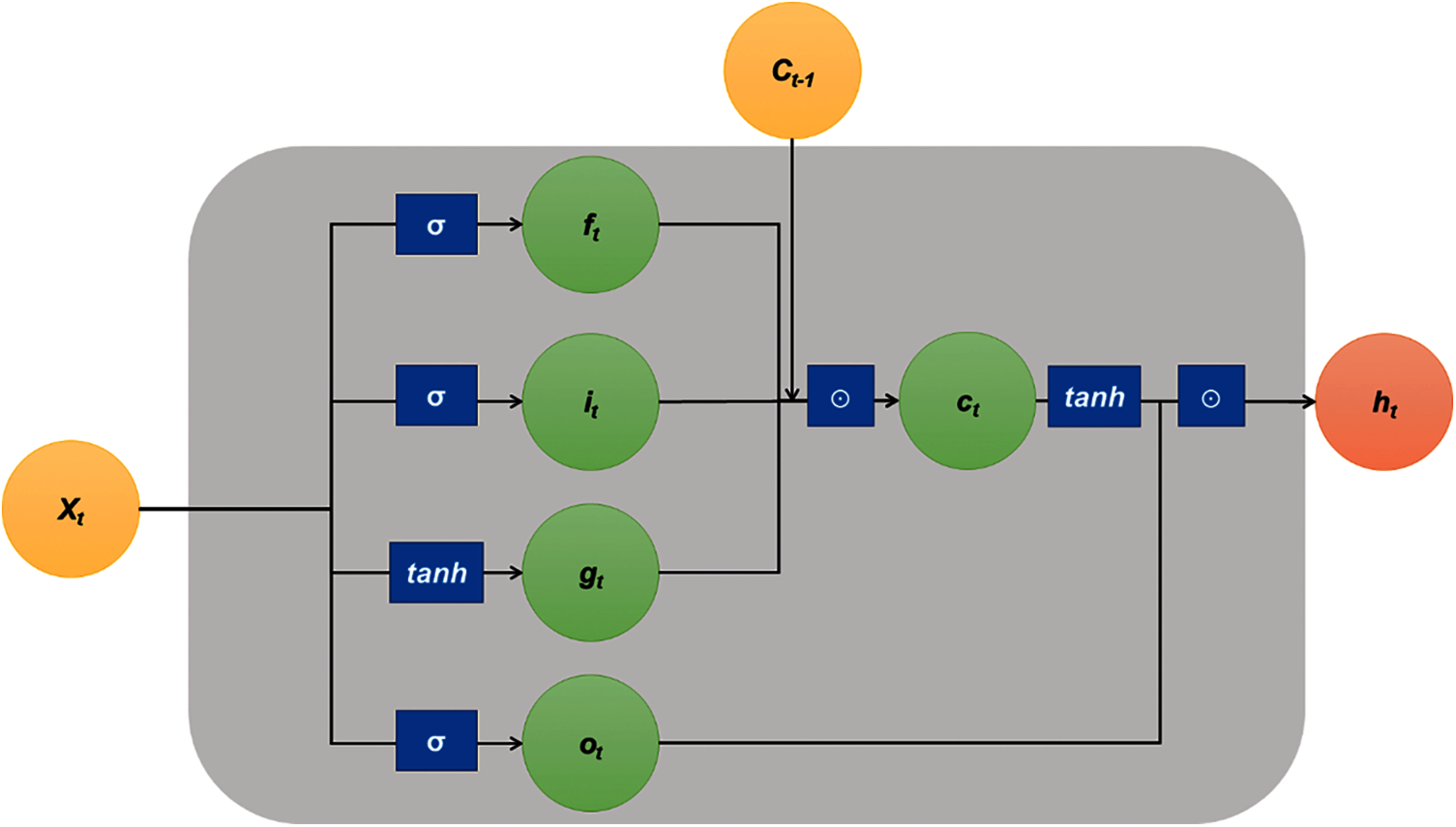
Figure 1: The modified schematic of the long short-term memory (LSTM) model network
The LSTM model has a disadvantage that as the number of training increases, the amount of computation increases, so it requires a lot of time and memory for calculation, and when the number of input data is insufficient, the learning accuracy is degraded. In order to improve these shortcomings, the GRU model in which the number of parameters is reduced by removing the output gate has been proposed, and the overall network is as Fig. 2.
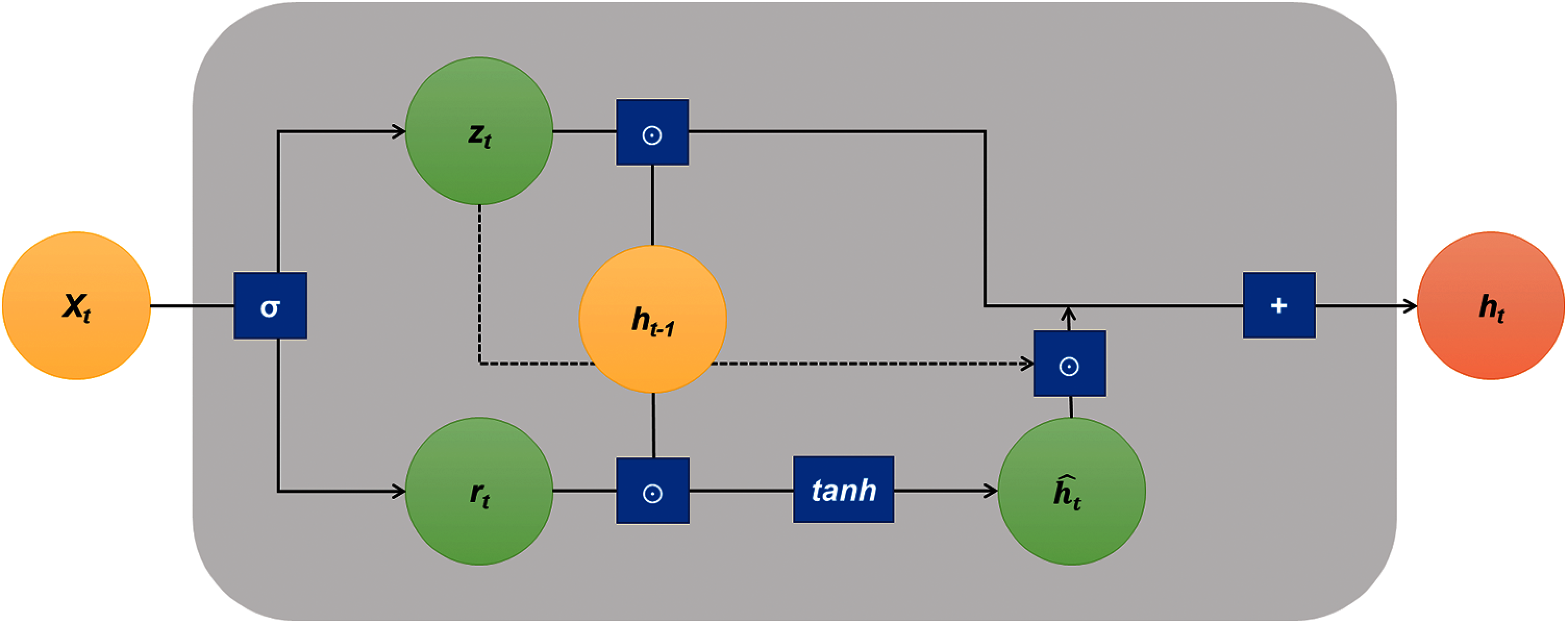
Figure 2: The modified schematic of the gated recurrent unit (GRU) model network
The GRU model consists of two gates (reset gate layer, update gate layer), and candidate activation is utilized. The overall calculation process of GRU is as follows [41].
where, zt is update gate vector, rt is reset gate vector, and
The first step of the GRU is to determine the information to be reflected and deleted through the sigmoid function, similar to the LSTM, and is carried out in the reset gate layer. The next step is to determine the update rate of the previous and the current information. The amount of current and previous information is settled by subtracting the data determined in the previous step, the reset gate layer. This method is similar to forget gate layer and input gate layer in LSTM [42]. Finally, the result of the candidate activation vector and the update gate vector is summed, and the result is output. The GRU model is one of the most widely used variant models because of its simpler structure and its faster learning speed than the LSTM model. Since both models have high performance and it is not known which model performs better, in this paper, both models were performed to find a model that can predict with higher accuracy. RNN stores previous learning values in a hidden layer (memory cells), and there is a limit in that the previously stored values are lost as the amount stored increases. The deep learning algorithms used in this paper, LSTM and GRU, are the same as RNN in that they store previous values, but use of stored values is erased through the forget gate to prevent memory limitations. The incremental learning methods have been used in consideration of the experimental tests, where data is continuously received, rapidly changed, and limited.
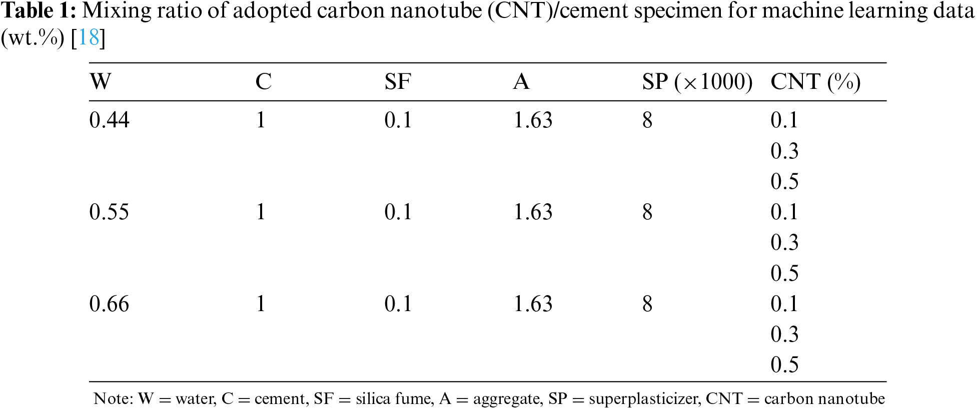
In this paper, experimental data were obtained through the results of previous kinds of literature [18,19]. The mixing ratio of the adopted CNT/cement specimens applied to the machine learning methods are listed in Tab. 1. It is noted that the data applied in this study are comprehensive values analyzed based on the appropriate number of specimens recommended by ASTM standards [18,19]. This is not a very large amount of data, but it is thought to be sufficient to discuss the generality of the experimental results. The experiment variables conducted by [18] are W/B, contents of CNTs, and curing conditions. The mixing ratio of the adopted CNT/cement specimens applied to the deep learning methods are listed in Tab 2. In the experimental data conducted by [19], W/B and CNT contents were fixed, and the internal relative humidity was set as an experimental variable to measure the specimen data accordingly. The specimens prepared in [18] were the W/B ratio, content of CNTs, and the curing temperature (oven dry; OD and saturated surface dry; SSD) as experimental variables, and the piezoelectric performance of these specimens was tested. Hence, it was classified into 18 experimental groups by three W/B ratios (0.3, 0.4, and 0.5), three MWCNT contents (0.1, 0.3, and 0.5 wt.%), and two curing conditions (OD and SSD). The extracted data sets consisted of 435 to 959 values [18]. The number of extracted data applied for each variable is as follows: W/B0.4-CNT0.1-SSD = 704, W/B0.4-CNT0.1-OD = 515, W/B0.5-CNT0.1-SSD = 681, W/B0.5-CNT0.1-OD = 554, W/B0.6-CNT0.1-SSD = 637, W/B0.6-CNT0.1-OD = 786, W/B0.4-CNT0.3-SSD = 482, W/B0.4-CNT0.3-OD = 435, W/B0.5-CNT0.3-SSD = 502, W/B0.5-CNT0.3-OD = 959, W/B0.6-CNT0.3-SSD = 607, W/B0.6-CNT0.3-OD = 868, W/B0.4-CNT0.5-SSD = 780, W/B0.4-CNT0.5-OD = 583, W/B0.5-CNT0.5-SSD = 547, W/B0.5-CNT0.5-OD = 569, W/B0.6-CNT0.5-SSD = 642, W/B0.6-CNT0.5-OD = 874.

In [19], repeated piezoelectric performance experiments were conducted with four types of samples having different internal relative humidity (D). The number of experimental data according to the four different values of D (55, 65, 70, and 85) is 376, 328, 366, and 424, respectively. In both experiments, the stress on the specimen was repeated for a predetermined cycle and measured using the 2-probe method. In this study, the time series data of the experimental results provided by the literate were cropped and used as data for learning and prediction. Especially, this paper focused on predicting fractional change in the electrical resistivity (FCR) based on the input variables: content of MWCNT, the internal relative humidity of the specimen, the W/B ratio, the compressive strength, and the time. The fabrication processes and material properties of MWCNT-embedded cement composites are described in detail in the reference kinds of literature [18,19].
The predicted results based on the abovementioned nine machine learning algorithms for all specimens are shown in Figs. 3 and 4, and Tab. 3. In these figures, the blue dot represents the experimental value, and the yellow dot signifies the predicted results. In addition, the X-axis of the graph means the applied stress, the Y-axis is the electric resistance change. The piezoelectric characteristic of CNT/cement composites is most sensitive near the percolation threshold. According to the existing literatures [1,4,6], the percolation threshold of CNT/cement composites is formed approximately 0.4 to 0.5 wt.%. Since a relatively small amount of CNTs (0.1 wt.%) was incorporated into the specimen, experimental data in Figs. 3a and 4a with W/B:0.4 exhibited unstable piezoelectric properties. Regardless of the curing conditions (OD and SSD) and CNT contents (0.1, 0.3, and 0.5 wt.%) of the specimen, GPR and GPTIPS showed the best predictive performances, and the average RMSE values were 0.0649 and 0.1356, respectively. The RMSE values were calculated through comparison with various machine learning techniques and experiments, resulting that GPTIPS method is the most accurate method. GPR method showed the second highest accuracy, but for the case of W/B 0.6 and CNT 0.1 wt.%, the RMSE value was 0.0199, which was the lowest value among all cases. The utilized dataset was the experimentally measured piezoelectric results of CNT/cement composites. The cement-based nanocomposites were manufactured by varying the amount of CNT contents, binder to CNTs ratio, curing conditions, and relative internal humidity. External stresses ranging from 0.25 to 12.12 MPa were applied to the specimens, and piezoelectric values derived therefrom were applied as training data.
Tab. 3 shows the RMSE values for each algorithm in Figs. 3 and 4, and the values in bold are the most outstanding result in this test. Since the uncertainty in the experimental dataset can be represented as mean and covariance in GPR, the estimation models with covariance function of squared exponential shows the best performance with the relatively small number of datasets. The GPTIPS which considers both the model predictive performance and model complexity by building nonlinear regression models also shows the most outstanding result in half of the cases.
The LSTM and GRU models are applied to predict the FCR of CNTs-embedded cementitious composites with varying internal relative humidity. The software used for the analysis was TensorFlow, and the applied LSTM model was BasicLSTMCell. The values of learning rate and epoch (iterative learning) were set to be 0.01 and 500, respectively. The computational time took approximately 3–5 h per one case. The input variables applied to the analysis were time, CNT content, W/B, curing condition, applied load, and internal relative humidity. The electrical resistivity change was considered for the output. The prediction performances were evaluated through the RMSE value that represents the difference between the actual value and the predicted result. In consideration of the amount of data, the running rate, batch size, and epoch (iterative learning) were set to 0.01, 4, and 500, respectively. In addition, 70% of the total data was used for training, and prediction was made based on the remaining 30% of the data. The estimation results and RMSE according to the number of epochs are represented in Fig. 5
Figs. 6 and 7 show the prediction results of FCR and RMSE based on the LSTM and GRU methods. Fig. 6 represents the prediction graphs for 30% of specimens having D = 55, 65, 70, and 85. In this figure, the X-axis indicates the time, the Y-axis represents the predicted FCR value. The red and green lines signify the actual value and predicted values. The predicted time-dependent piezoelectric responses are shown to be a good agreement with the experimental data. Particularly, the accuracy of the predictions was not significantly different between LSTM and GRU methods.
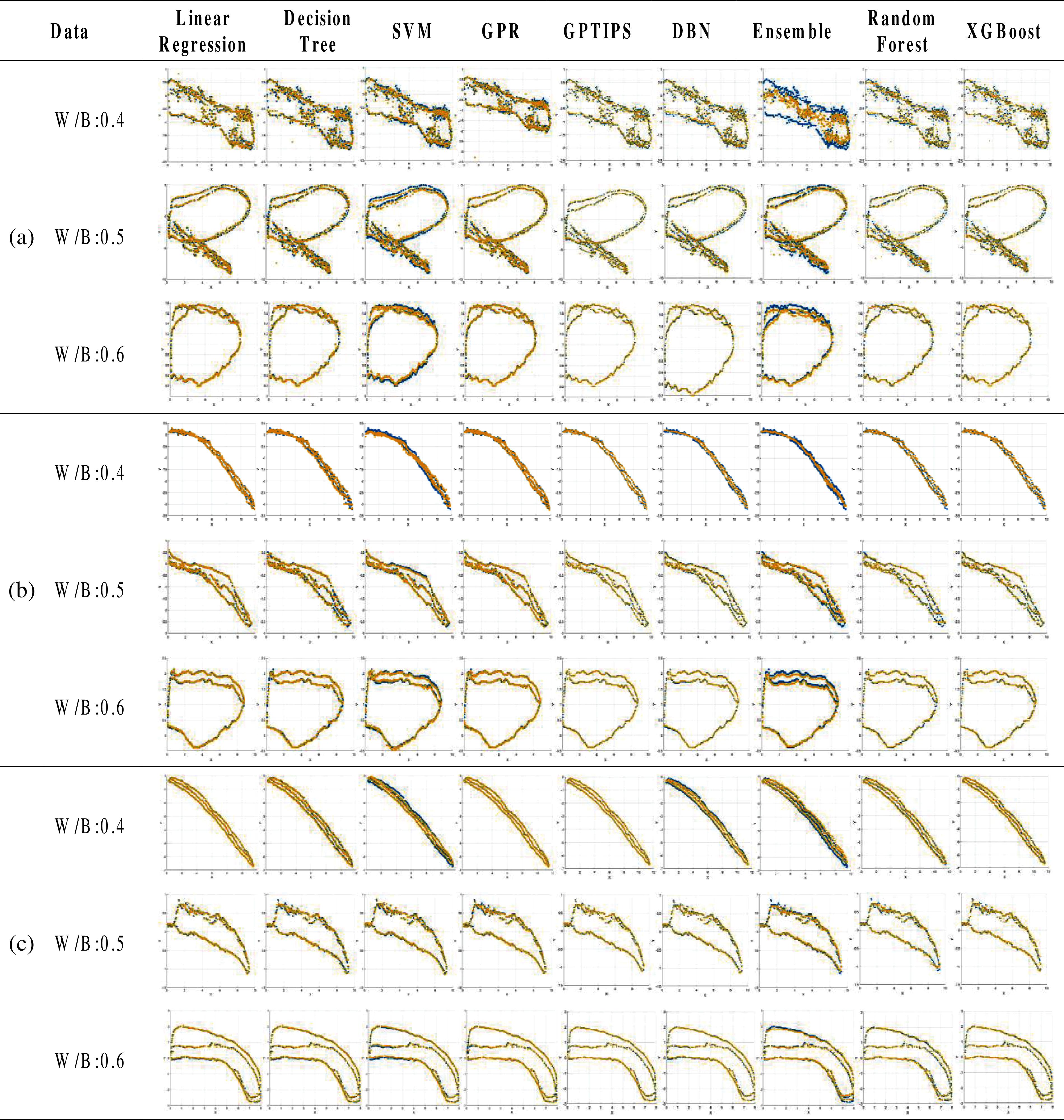
Figure 3: Analysis through machine learning algorithms in SSD specimens with various CNT content: (a) 0.1, (b) 0.3, and (c) 0.5 wt.%
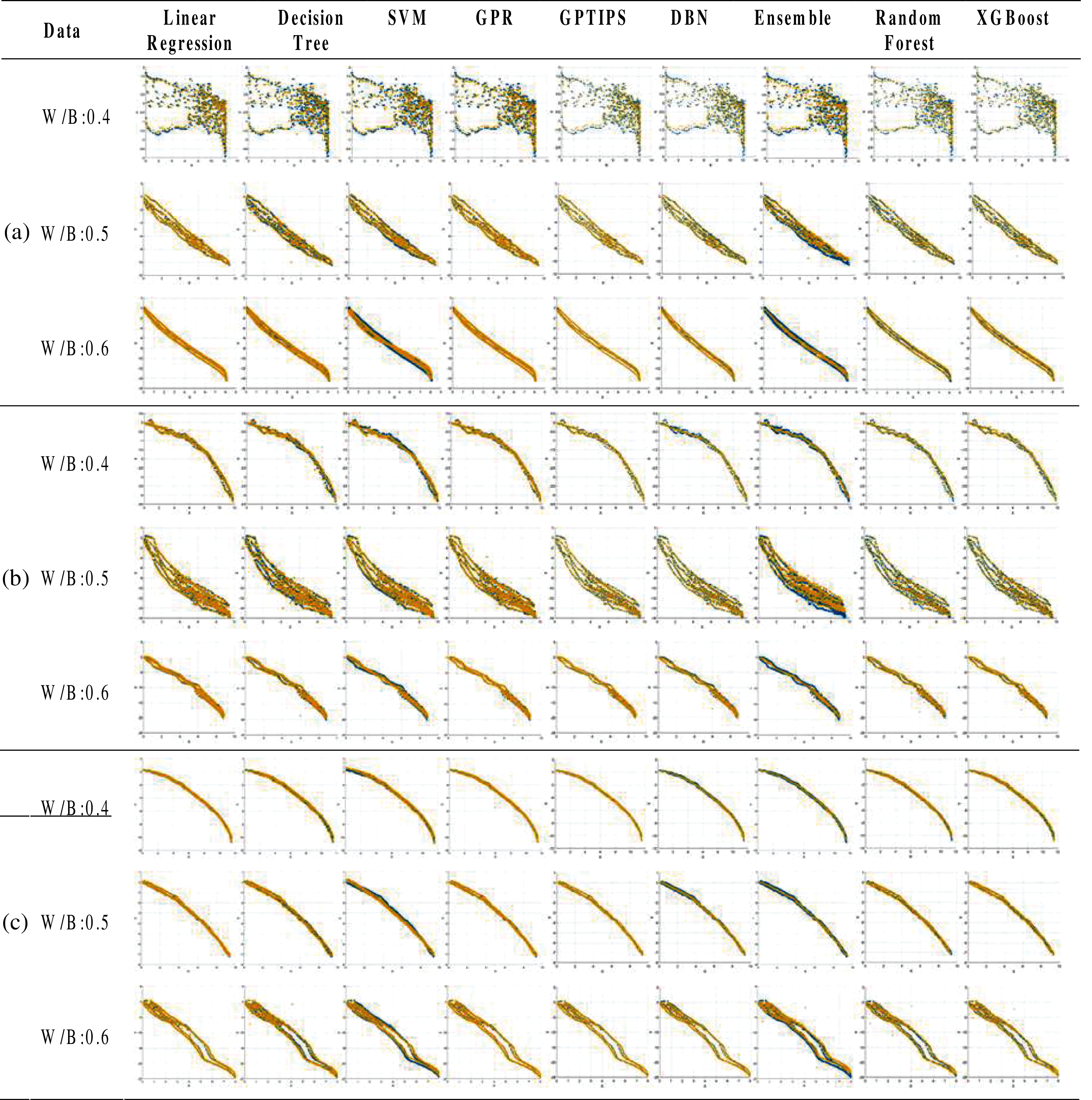
Figure 4: Analysis through machine learning algorithms in OD specimens with various CNT content: (a) 0.1 wt.%, (b) 0.3 wt.%, and (c) 0.5 wt.%
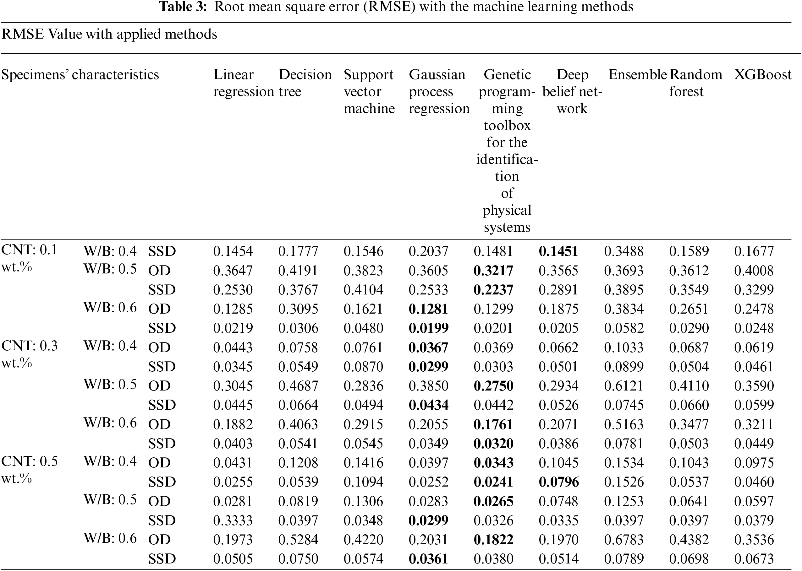

Figure 5: (a) An overview of this study that uses 70% of the data for training and 30% of the data for prediction, (b) analysis results of entire data, (c) the enlarged portion of the predicted value, and (d) the RMSE of the simulation results
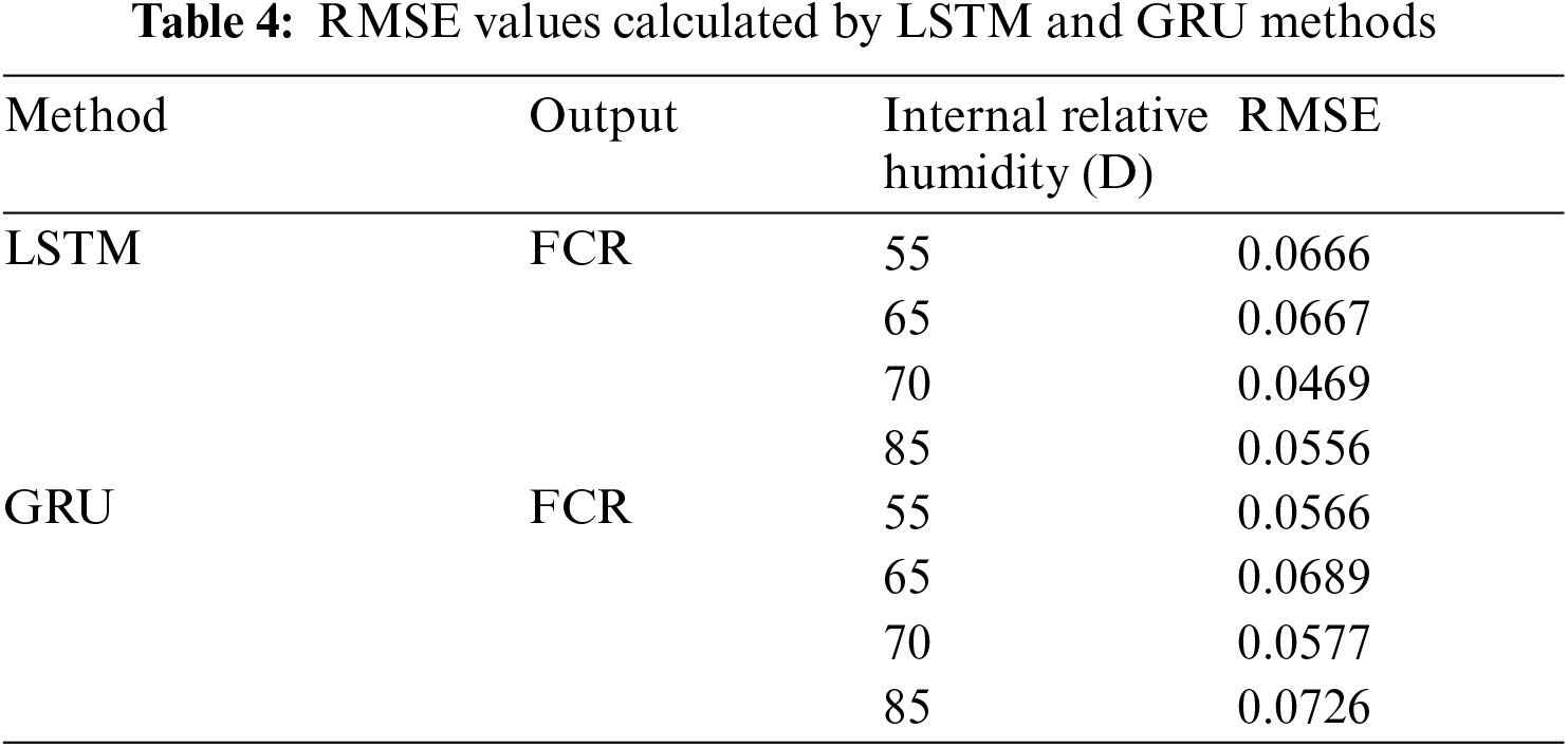
The RMSE values given in Figs. 6 and 7 are listed in Tab. 4. In GRU, the weights required for training is reduced and the computational load is reduced, as the network of LSTM is simplified. The average RMSE value calculated by the LSTM method was 0.059, and the value calculated based on the GRU method was 0.064. The RMSE value calculated by GRU method was higher than that of LSTM. However, the magnitude of the value is very small and the difference between the results is insignificant, which is not an appropriate value to judge the superiority of the prediction method. The calculation time with the GRU shows slightly faster in comparison with the prediction through the LSTM, since the GRUs have fewer parameters to update and need less data to generalize.
It can be seen from Tab. 4 that both LSTM and GRU methods that analyze and predict sequential data show quite accurate results. It is attributed to the fact that the sequential data applied to this piezoelectric analysis are fairly stable and have predictable period. Therefore, it is judged that the accuracy of this model can be analyzed more comprehensively by applying the data including the nonlinear or fracture behavior of the material. This is beyond the scope of this study, but it is planned to proceed in this direction in the future. The methodology conducted in the present study has a limitation in that it is the result of the selected environment and material combination. Therefore, different results could be deduced when other types of ceramic matrix (e.g., Types II-V of cement, silicon carbide, and alkali-activated material) or nano-fillers (graphene, boron nitride nanotube, nanoparticle etc.) are applied. Considering all kinds of materials is a limitation beyond the scope of this study, which will be validated through future study.
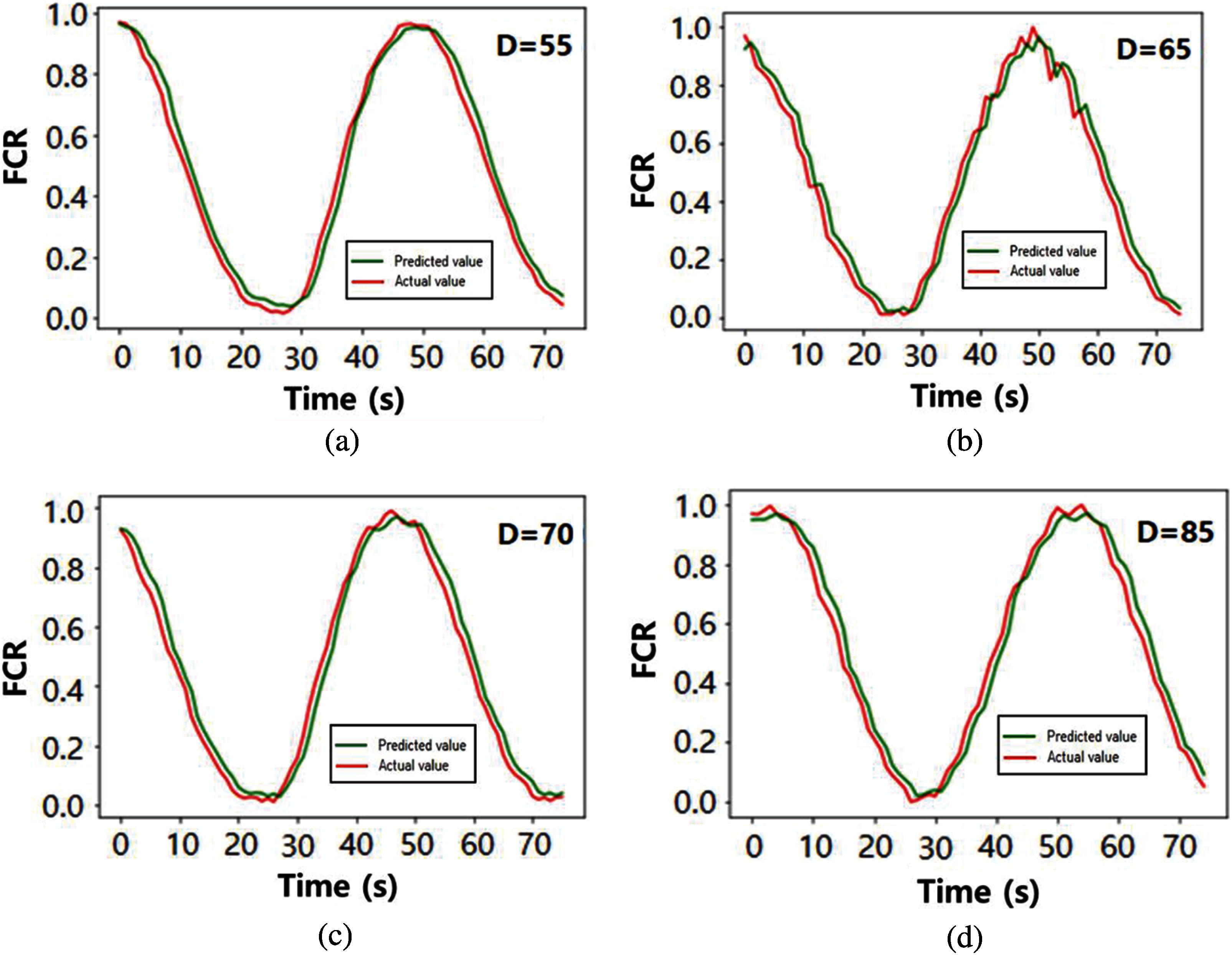
Figure 6: The predicted results based on LSTM: (a) internal relative humidity (D) = 55, (b) D = 65, (c) D = 70, and (d) D = 85
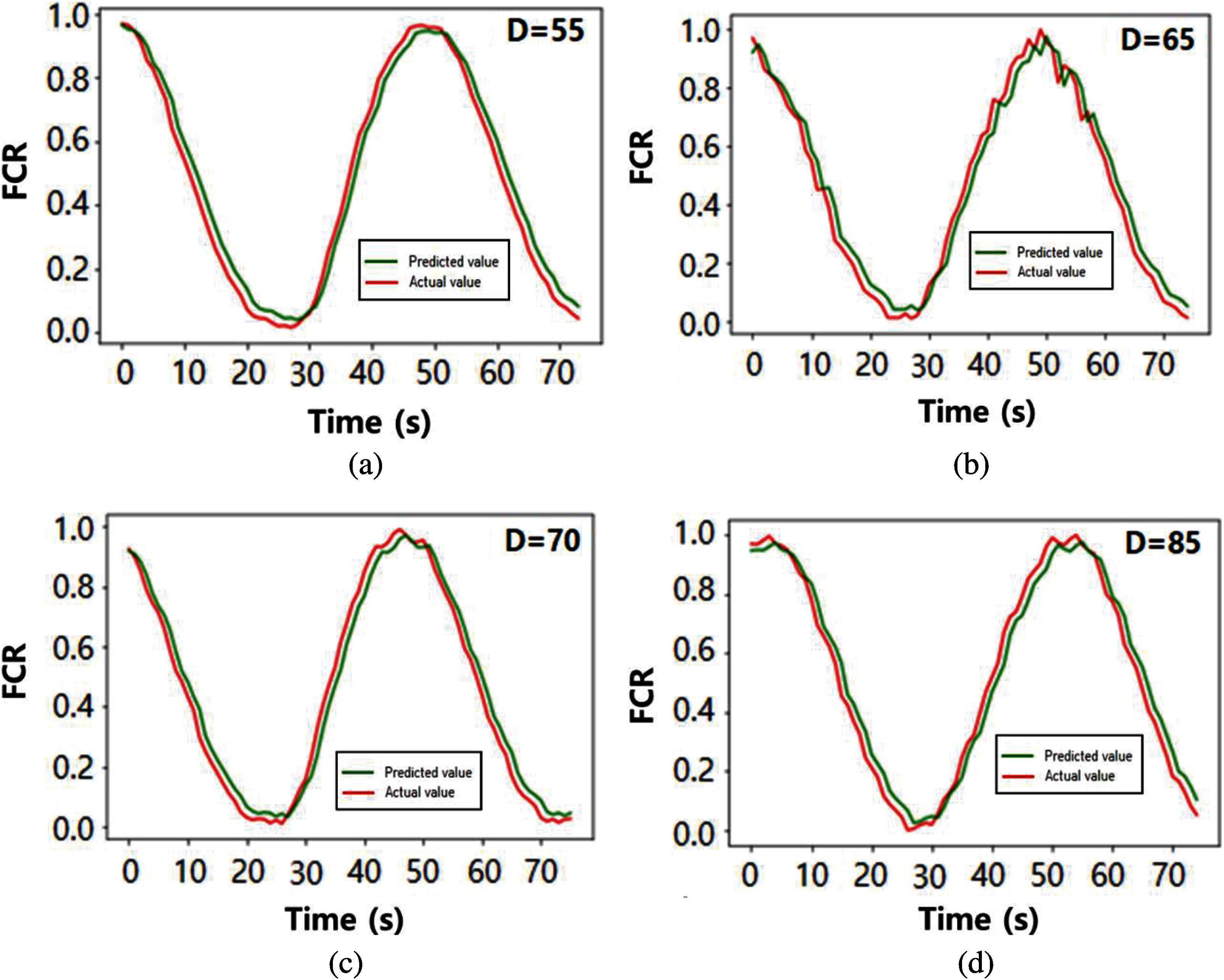
Figure 7: The predicted results based on GRU: (a) D = 55, (b) D = 65, (c) D = 70, and (d) D = 85
Herein, we proposed a machine learning based methodology considering material constituent of electrical cement-based composites with CNTs. Different approaches were considered to evaluate the piezoelectric properties of specimens that were not time-dependent and depended. The effectiveness of the proposed methodologies was validated by comparing experimental data in the literature, and the key findings thus obtained are summarized below.
(1) In the analysis of piezoelectric performance of specimens under static loading condition, it was confirmed that the GPR and GPTIPS show the better accuracy.
(2) The difference between LSTM and GRU in estimating piezoelectric performance with time-history was not very large in this study.
(3) The curve of resistivity change by dynamics loading is very monotonous, and it would have been insufficient to lead the difference in the analysis results.
(4) Since the cement matrix undergoes a hydration reaction over a long period of time, it is considered appropriate to proceed in the direction of considering the effect on time.
We believe that the proposed methodologies, consisting of two approaches, enables precise predictions of functional inhomogeneous cementitious composites on relatively large scale with considerably reduced computational time.
Funding Statement: The authors received no specific funding for this study.
Conflicts of Interest: The authors declare that they have no conflicts of interest to report regarding the present study.
1. G. Kim, I. Nam, B. Yang, H. Yoon, H. K. Lee et al., “Carbon nanotube (CNT) incorporated cementitious composites for functional construction materials: The state of the art,” Composite Structures, vol. 227, p. 111244, 2019. [Google Scholar]
2. V. L. Kuznetsov and P. P. Edwards, “Functional materials for sustainable energy technologies: Four case studies,” Chemistry & Sustainability Energy & Materials, vol. 3, no. 1, pp. 44–58, 2010. [Google Scholar]
3. B. Yang, K. Cho, G. Kim and H. K. Lee, “Effect of CNT agglomeration on the electrical conductivity and percolation threshold of nanocomposites: A micromechanics-based approach,” Computer Modeling in Engineering & Sciences, vol. 103, no. 5, pp. 343–365, 2014. [Google Scholar]
4. A. Mohammed, J. G. Sanjayan, W. Duan and A. Nazari, “Incorporating graphene oxide in cement composites: A study of transport properties,” Construction and Building Materials, vol. 84, pp. 341–347, 2015. [Google Scholar]
5. A. Thomas, “Functional materials: From hard to soft porous frameworks,” Angewandte Chemie International Edition, vol. 49, no. 45, pp. 8328–8344, 2010. [Google Scholar]
6. A. P. Singh, B. K. Gupta, M. Mishra, A. Chandra, R. Mathur et al., “Multiwalled carbon nanotube/cement composites with exceptional electromagnetic interference shielding properties,” Carbon, vol. 56, pp. 86–96, 2013. [Google Scholar]
7. R. Nadiv, M. Shtein, M. Refaeli, A. Peled and O. Regev, “The critical role of nanotube shape in cement composites,” Cement and Concrete Composites, vol. 71, pp. 166–174, 2016. [Google Scholar]
8. G. Kim, B. Yang, H. Yoon and H. K. Lee, “Synergistic effects of carbon nanotubes and carbon fibers on heat generation and electrical characteristics of cementitious composites,” Carbon, vol. 134, pp. 283–292, 2018. [Google Scholar]
9. G. Giannopoulos, S. Georgantzinos, D. Katsareas and N. Anifantis, “Numerical prediction of young's and shear moduli of carbon nanotube composites incorporating nanoscale and interfacial effects,” Computer Modeling in Engineering & Sciences, vol. 56, no. 3, pp. 231–247, 2010. [Google Scholar]
10. J. Wang, L. Zhang and K. Liew, “A multiscale modeling of CNT-reinforced cement composites,” Computer Methods in Applied Mechanics and Engineering, vol. 309, pp. 411–433, 2016. [Google Scholar]
11. J. Wang, L. Zhang and K. Liew, “Multiscale simulation of mechanical properties and microstructure of CNT-reinforced cement-based composites,” Computer Methods in Applied Mechanics and Engineering, vol. 319, pp. 393–413, 2017. [Google Scholar]
12. M. Eftekhari, S. H. Ardakani and S. Mohammadi, “An XFEM multiscale approach for fracture analysis of carbon nanotube reinforced concrete,” Theoretical and Applied Fracture Mechanics, vol. 72, pp. 64–75, 2014. [Google Scholar]
13. B. F. Haile, D. Jin, B. Yang, S. Park and H. K. Lee, “Multi-level homogenization for the prediction of the mechanical properties of ultra-high-performance concrete,” Construction and Building Materials, vol. 229, p. 116797, 2019. [Google Scholar]
14. F. Ye, “Particle swarm optimization-based automatic parameter selection for deep neural networks and its applications in large-scale and high-dimensional data,” Plos One, vol. 12, no. 12, pp. e0188746, 2017. [Google Scholar]
15. J. Neggers, O. Allix, F. Hild and S. Roux, “Big data in experimental mechanics and model order reduction: Today's challenges and tomorrow's opportunities,” Archives of Computational Methods in Engineering, vol. 25, no. 1, pp. 143–164, 2018. [Google Scholar]
16. F. H. Chiew, C. K. Ng, K. C. Chai and K. M. Tay, “A fuzzy adaptive resonance theory-Based model for Mix proportion estimation of high-Performance concrete,” Computer-Aided Civil and Infrastructure Engineering, vol. 32, no. 9, pp. 772–786, 2017. [Google Scholar]
17. H. M. Park, S. Park, S. M. Lee, I. J. Shon, H. Jeon et al., “Automated generation of carbon nanotube morphology in cement composite via data-driven approaches,” Composites Part B: Engineering, vol. 167, pp. 51–62, 2019. [Google Scholar]
18. H. Kim, I. Park and H. K. Lee, “Improved piezoresistive sensitivity and stability of CNT/cement mortar composites with low water–binder ratio,” Composite Structures, vol. 116, pp. 713–719, 2014. [Google Scholar]
19. C. Song and S. Choi, “Moisture-dependent piezoresistive responses of CNT-embedded cementitious composites,” Composite Structures, vol. 170, pp. 103–110, 2017. [Google Scholar]
20. D. C. Montgomery, E. A. Peck and G. G. Vining, In Introduction to Linear Regression Analysis, 4th ed., John Wiley & Sons, New Jersey, USA, 2012. [Google Scholar]
21. A. H. Khan, M. A. Khan, S. Abbas, S. Y. Siddiqui, M. A. Saeed et al., “Simulation, modeling, and optimization of intelligent kidney disease predication empowered with computational intelligence approaches,” Computers Materials & Continua, vol. 67, no. 2, pp. 1399–1412, 2021. [Google Scholar]
22. A. J. Myles, R. N. Feudale, Y. Liu, N. A. Woody and S. D. Brown, “An introduction to decision tree modeling,” Journal of Chemometrics, vol. 18, no. 6, pp. 275–285, 2004. [Google Scholar]
23. S. Suthaharan, Machine Learning Models and Algorithms for big Data Classification, 1st ed., Springer, Boston, MA, USA, pp. 1–12, 2016. [Google Scholar]
24. W. S. Noble, “What is a support vector machine?,” Nature Biotechnology, vol. 24, no. 12, pp. 1565–1567, 2006. [Google Scholar]
25. N. Tabassum, A. Ditta, T. Alyas, S. Abbas, H. Alquhayz et al., “Prediction of cloud ranking in a hyperconverged cloud ecosystem using machine learning,” Computers Materials & Continua, vol. 67, no. 3, pp. 3129–3141, 2021. [Google Scholar]
26. C. E. Rasmussen, “Gaussian processes in machine learning,” In Advanced Lectures on Machine Learning, Springer, Berlin, Heidelberg, Germany, pp. 63–71, 2003. [Google Scholar]
27. D. Opitz and R. Maclin, “Popular ensemble methods: An empirical study,” Journal of Artificial Intelligence Research, vol. 11, pp. 169–198, 1999. [Google Scholar]
28. D. P. Searson, D. E. Leahy and M. J. Willis, “GPTIPS: an open source genetic programming toolbox for multigene symbolic regression,” in Proc. Int. Multiconference of Engineers and Computer Scientists, Hong Kong, pp. 77–80, 2010. [Google Scholar]
29. Y. Hua, J. Guo and H. Zhao, “Deep belief networks and deep learning,” in Proc. 2015 Int. Conf. on Intelligent Computing and Internet of Things, Harbin, China, pp. 1–4, 2015. [Google Scholar]
30. M. Anam, V. Ponnusamy, M. Hussai, M. W. Nadeem, M. Javed et al., “Osteoporosis prediction for trabecular bone using machine learning: A review,” Computers Materials & Continua, vol. 67, no. 1, pp. 89–105, 2021. [Google Scholar]
31. S. S. Aralikatti, K. N. Ravikumar, H. Kumar, H. S. Nayaka and V. Sugumaran, “Comparative study on tool fault diagnosis methods using vibration signals and cutting force signals by machine learning technique,” Structural Durability & Health Monitoring, vol. 14, no. 2, pp. 127–145, 2020. [Google Scholar]
32. M. V. Madhavan, D. N. H. Thanh, A. Khamparia, S. Pande, R. Malik et al., “Recognition and classification of pomegranate leaves diseases by image processing and machine learning techniques,” Computers Materials & Continua, vol. 66, no. 3, pp. 2939–2955, 2021. [Google Scholar]
33. N. Naheed, M. Shaheen, S. A. Khan, M. Alawairdhi and M. A. Khan, “Importance of features selection, attributes selection, challenges and future directions for medical imaging data: A review,” Computer Modeling in Engineering & Sciences, vol. 125, no. 1, pp. 314–344, 2021. [Google Scholar]
34. A. Graves, A. R. Mohamed and G. Hinton, “Speech recognition with deep recurrent neural networks,” in Proc. ICASSP 2013, Vancouver, Canada, pp. 6645–6649, 2013. [Google Scholar]
35. A. Graves, In Supervised Sequence Labelling with Recurrent Neural Networks, 1st ed., Springer, Berlin, Heidelberg, Germany, 2012. [Google Scholar]
36. J. Chung, C. Gulcehre, K. Cho and Y. Bengio, “Empirical evaluation of gated recurrent neural networks on sequence modeling,” in NIPS 2014 Workshop on Deep Learning, Montreal, Canada, 2014. [Google Scholar]
37. Y. Bengio, P. Simard and P. Frasconi, “Learning long-term dependencies with gradient descent is difficult,” IEEE Transactions on Neural Networks, vol. 5, no. 2, pp. 157–166, 1994. [Google Scholar]
38. M. A. Khan and Y. Kim, “Deep learning-based hybrid intelligent intrusion detection system,” Computers Materials & Continua, vol. 68, no. 1, pp. 671–687, 2021. [Google Scholar]
39. S. Hochreiter and J. Schmidhuber, “Long short-term memory,” Neural Computation, vol. 9, no. 8, pp. 1735–1780, 1997. [Google Scholar]
40. A. Shewalkar, “Performance evaluation of deep neural networks applied to speech recognition: RNN, LSTM and GRU,” Journal of Artificial Intelligence and Soft Computing Research, vol. 9, no. 4, pp. 235–245, 2019. [Google Scholar]
41. N. Boulanger-Lewandowski, Y. Bengio and P. Vincent, “Modeling temporal dependencies in high-dimensional sequences: application to polyphonic music generation and transcription,” in Proc. 29th Int. Conf. on Int. Conf. on Machine Learning, Edinburgh, UK, pp. 1881–1888, 2012. [Google Scholar]
42. K. Cho, B. Van Merriënboer, C. Gulcehre, D. Bahdanau, F. Bougares et al., “Learning phrase representations using RNN encoder-decoder for statistical machine translation,” in Proc. EMNLP, Doha, Qatar, pp. 1724–1734, 2014. [Google Scholar]
 | This work is licensed under a Creative Commons Attribution 4.0 International License, which permits unrestricted use, distribution, and reproduction in any medium, provided the original work is properly cited. |