Computers, Materials & Continua DOI:10.32604/cmc.2022.021441
Article

Energy-Efficient Resource Optimization for Massive MIMO Networks Considering Network Load

Samira Mujkic1,*, Suad Kasapovic1 and Mohammed Abuibaid2

1Department of Telecommunications, Faculty of Electrical Engineering, University of Tuzla, Tuzla, 75000, Bosnia and Herzegovina
2Department of Systems and Computer Engineering, Faculty of Engineering and Design, Carleton University, Ottawa, K1S 5B6, Canada
*Corresponding Author: Samira Mujkic. Email: samira.mujkic@unitz.ba
Received: 03 July 2021; Accepted: 30 August 2021

Abstract: This paper investigates the resource optimization problem for a multi-cell massive multiple-input multiple-output (MIMO) network in which each base station (BS) is equipped with a large number of antennas and each base station (BS) adapts the number of antennas to the daily load profile (DLP). This paper takes into consideration user location distribution (ULD) variation and evaluates its impact on the energy efficiency of load adaptive massive MIMO system. ULD variation is modeled by dividing the cell into two coverage areas with different user densities: boundary focused (BF) and center focused (CF) ULD. All cells are assumed identical in terms of BS configurations, cell loading, and ULD variation and each BS is modeled as an M/G/m/m state dependent queue that can serve a maximum number of users at the peak load. Together with energy efficiency (EE) we analyzed deployment and spectrum efficiency in our adaptive massive MIMO system by evaluating the impact of cell size, available bandwidth, output power level of the BS, and maximum output power of the power amplifier (PA) at different cell loading. We also analyzed average energy consumption on an hourly basis per BS for the model proposed for data traffic in Europe and also the model proposed for business, residential, street, and highway areas.

Keywords: Massive MIMO; traffic load; energy efficiency; user location distribution; optimization

1  Introduction

In the current mobile communication systems, due to the technical limits such as occupied space and implementation complexity in a multi-antenna system, the number of antennas configured on the transmitter/receiver (TX/RX) end is limited. Massive MIMO has been recently proposed as a potential technique that significantly enables the increase the network throughput and energy efficiency [1,2].

The amount of mobile data traffic has increased dramatically over the years, which is mainly driven by the massive demand of data-hungry devices such as smart phones, tablets and broadband wireless applications such as multimedia, three-dimensional (3D) video games, e-Health, Car2X communications [3]. In particular, the radio access part of the wireless cellular network is a major energy killer, which accounts for up to more than 70% of the total energy bill [4]. Also, the Carbon dioxide (CO2) contribution of the telecommunications sector to the global CO2 emission has increased rapidly over the last decade, where mobile operators are among the top energy consumers. Thus, besides spectral efficiency, energy efficiency is crucial, so wireless researchers and engineers need to shift their focus to energy-efficiency oriented design in order to reduce the operation cost for mobile operators and minimize the environmental impact of the wireless domain.

In general, efficient allocation of radio resources (e.g., power, frequency, time, and antennas) plays a crucial role in improving wireless network performance. Taking into consideration different points of view, there are several energy efficiency (EE) metrics to evaluate wireless networks. In particular, authors at [5] are bringing new insights into how the M number of antennas at the base station (BS), the number K of active user equipment (UEs), and the transmit power must be chosen to uniformly cover a given area with maximal EE. In [2] authors focused in the design of a green, highly energy-efficient cellular heterogeneous network (HetNet) by taking advantage of MIMO structure and deployment of small cells. Authors have furthermore designed a joint antenna selection and Resource Block (RB) allocation algorithm, followed by a power optimization algorithm, to maximize the system EE under the additional constraints of minimum guaranteed user rates and maximum fronthaul capacity limits.

Resource allocation for EE maximization has been an active area of research in recent years. Design of an optimal resource allocation algorithm can be challenging especially if the underlying resource allocation problems are non-convex [6]. Previous related contributions have already provided some insights into energy-efficient systems design with load-adaptive massive MIMO.

Furthermore, several works [7] the authors optimized power amplifiers (PA) dimensioning for massive MIMO systems with load adaptive number of antennas. Their study considers both the traditional PA (TPA) and a more efficient PA, namely envelope tracking PA (ET-PA). An iteration optimization algorithm was proposed in [8] for a multi-cell massive MIMO system where each cell maximizes average EE adaptively with the variation of network load. The proposed algorithm yields significant gains in EE at the cost of reduction of average user data rate at low user load. Our results show that, EE and average user rate (UR), increase or decrease with the change of certain system parameters. EE maximization problem in [9] is formulated in a game theoretic framework where the number of antennas, which will be used by a BS, is determined by best response iteration. This load adaptive system achieves an overall 19% higher EE compared to a baseline system where the BSs always run with a fixed number of antennas. The impact of user location distribution (ULD) variation on the energy efficiency of a load-adaptive massive MIMO system is analyzed in [10]. The authors in [11] analyzed energy-efficient massive MIMO system focused on joint antenna selection, optimal transmit power, joint user selection, and circuit power consumption (CPC) to balance the radiated EE and adjust the length of the pilot sequences to improve channel estimation. In [12] authors developed a new parallel algorithm for resource allocation and subcarrier assignment, and implement the Hungarian algorithm on parallel architectures. However, none of these studies provided any mechanism for dealing with daily load changes and the impact of individual system parameters on EE, in a multi-cell scenario with different ULD models.

In this paper, the aim is to investigate the energy-efficient resource allocation algorithm for a single-cell and multi-cell multi-user massive MIMO system. Our paper examines the effect of two ULD models, namely, boundary focused (BF) and center focused (CF) and is different from [10] by analyzing the impact of cell size, available bandwidth, the output power level of the BS, and maximum output power of the PA on EE at different cell loading. The influence of certain mentioned system parameters was analyzed in similar works, but not on the system which has formed different ULD models. Also the influence of bandwidth size on performance was not analyzed in available papers on the same or similar system model. We propose a resource allocation strategy to adapt the number of antennas based on tracking variations of ULD and cell loading maximizing the EE. Resource allocation scheme jointly optimizes the number of BS antennas, user load distribution, and cell loading. This strategy is different from [8] by way of its taking advantage of two environment variations to exploit massive MIMO favorable propagation to lower the number of active antennas while maintaining a tolerable user rate loss and thus operating more efficiently.

In order to maximize EE throughout 24-hour operation of the network, it is necessary to optimize M following the daily load profile (DLP) and ULD model. In order to map the user distribution to the DLP, we model each BS as a state dependent M/G/m/m queue [13,14] and utilize the DLP as suggested in [15].

The above mentioned state dependency is due to the fact that the user rate depends on the number of users that the BS can serve simultaneously. The peak load of the DLP is when BS serves a maximum number of users. Network is dimensioned to handle peak data traffic and it becomes most energy efficient when serving maximum load.

In particular, we divide a cell into two areas and for each area, we consider the user distribution and the optimum number of antennas that maximize EE under the given network load and interference condition for any number of users a cell serves. Generally, a user located at the cell boundary will receive the weakest signals from its BS but the strong interference from other BSs. For this reason, our goal is to determine and compare system performance in these two cell areas.

The specific contributions of the paper are as follows:

•   We derive two systems for analyzing energy efficiency: adaptive and fixed antenna system, each one contains two ULD models boundary focused (BF) and center focused (CF).

•   We investigate the total energy efficiency of our considered and fixed antenna system taking into account the number of BS antennas, user load distribution, and cell loading.

•   We propose a dynamic resource allocation strategy to adapt the number of antennas based on tracking variations of user location distribution and cell loading.

The following section presents description of created models: system, ULD, traffic, and power consumption model. The third section provides a problem formulation and description of the created optimization algorithm. In the fourth part additional scenarios of the basic model are formed to ascertain which system parameter values of the analyzed model result in the best performance during the appliance of the massive MIMO. The results and the discussion of the analyses are also shown in the fourth part. At the end of the paper there is a conclusion.

2  Analyzed Models

In this paper, we consider a downlink of a multi-cell massive MIMO system that contains hexagonal cells, each having its own BS and we apply classic wrap-around to avoid edge effects. Each BS transmits a constant output power Pc and uses Mi antennas to serve Ki single-antenna users, such that Mi>Ki. Users with multiple antennas are not considered because of computation complexity, which UE has to pay to gain the benefit of multiple antennas. The users are distributed inside each cell according to created ULD models. Output power Pc at each BS is distributed equally among PAs, where each PA is connected to one antenna element, so, the mean output transmission power per antenna is p=Pc/Mi. We consider block flat-fading Rayleigh channel with Bc(Hz) coherence bandwidth and Tc (s) coherence time which remain static within a time-frequency coherence block of U=BcTc symbols. Spacing between adjacent antennas at the BS is such that the channel components between the BS antennas and the single-antenna UEs are uncorrelated and the path distances are the same. This is reasonable since the distances between UEs and the BS are much larger than the distance between array elements. Large-scale fading is dominated by path-loss and a typical 3rd Generation Partnership Project (3GPP) distance dependent path-loss model is used.

We assume that all BSs and UEs are synchronized and operate on time-division duplex (TDD) protocol and that the BS obtains perfect Channel state information (CSI) from the uplink pilots, which is a reasonable assumption for low-mobility scenarios. All BSs employ zero-forcing (ZF) precoding to cancel out intra-cell interference by using the beamforming technique, which is a signal processing technique that cancels out intra-cell interference by beamforming and adapts the power allocation to guarantee the same rate to each user. Numerical results in [16] show that ZF performs similarly to the close-to-optimal regularized zero-forcing precoding (RZF) scheme. ZF method requires the operation of direct matrix inversion and due it complexity authors in [17] proposed Weighted Gauss-Seidel (WGS) method to perform the ZF precoder and provides better error performance in spatially correlated channels. The authors of [18] have proposed flexible beamforming (FBF) antenna architecture that allows flexibility in terms of data rates, coverage and scalability in an energy efficient manner.

The energy-efficiency (in bits/Joule) of a massive MIMO system is defined in [19,20] as the spectral-efficiency (sum-rate in Mbit/s) divided by the total consumed power (in Joule/s). According to expression for rate and consumed power the corresponding EE will be:

EE(Ki,Mi)=∑k=1Kmax⁡R(k,Mi,)Pitotal(Ki,Mi)(1)

In the expression for distance-dependent rate at UEz, necessary overhead for channel acquisition in equal to Q1=(1−αKmaxTcBc), where α is the pilot reuse factor, Kmax is the maximum number of users assumed to be the same for all cells (i.e., the number of pilot sequences = αKmax) and TcBc is the number of channel uses that the channel stays fixed. Mean transmit power per user is Q2=pMiKi and Q3=(Mi−Ki) is the effective array gain. Average noise power that disturbs the received signal from the serving BS is expressed as Q4=Bδ2di(UEz) whereas Q5=∑j=1J⁡{dj(UEz)di(UEz)pMj} is average inter-cell interference power. The term di(UEz) in Q5 represents the path loss from the serving BS at origin cell i to UEz and the term dj(UEz) represents the path loss from interfering cell j to UEzinside the origin cell i. The distance-dependent rate at UEz within cell i can be found by:

RUEz(Ki)=BQ1log2(1+Q2Q3Q4+Q5)(2)

Power consumed in a BS depends on the number of active antennas and the number of users served simultaneously. It consists of a fixed part (e.g., control signal, backhaul, direct current-direct current (DC--DC) conversion) and a dynamic part, i.e., radiated transmit power and circuit power which depends on the number of active antennas and number of users served simultaneously.

Based on the models and the practical numbers in [21,22], the total power in a BS i with Mi active antennas and Ki users is given by:

Pitotal(Ki,Mi)=MiPPA(p)+PBB(Ki,Mi)+Poth(3)

where PPA(p) gives the power consumption of a traditional PA (TPA) when the average output power is p. The total input power needed by TPA can be approximated as [23,24]:

PPA(p)≈1ηp∗Pmax,PA(4)

where ηis the maximum TPA efficiency and Pmax,PA is maximum output power.

PBB(Ki,Mi) is the base band signal processing power when the BS serves Ki users simultaneously with Mi antennas. Poth includes the load-independent power for site cooling, control signal, DC--DC conversion loss, etc.

PBB(Ki,Mi)=∑k=1Kmax⁡Ri(k)(PCOD+PDEC)+Psyn+BKi33TcLBS+PBS+BKiLBS(2+1TC)+3BKi2LBS(5)

where ∑k=1Kmax⁡Ri(k) is the total rate handled by the BS as calculated in Eq. (2), PCOD and PDEC are the power required for coding and decoding, respectively, whereas Psyn is the power consumed by the local oscillator. LBS is BSi computational efficiency. PBS is the power required to run the circuit components, e.g., converters, mixers and filters attached to each antenna at the BS.

ULD model formed in this paper defines two coverage areas which are divided with radius rD, so that rD>rmin and rD<rmax. Fig. 1 shows how cell is divided into two coverage areas, for the case of rmax=1000 m.

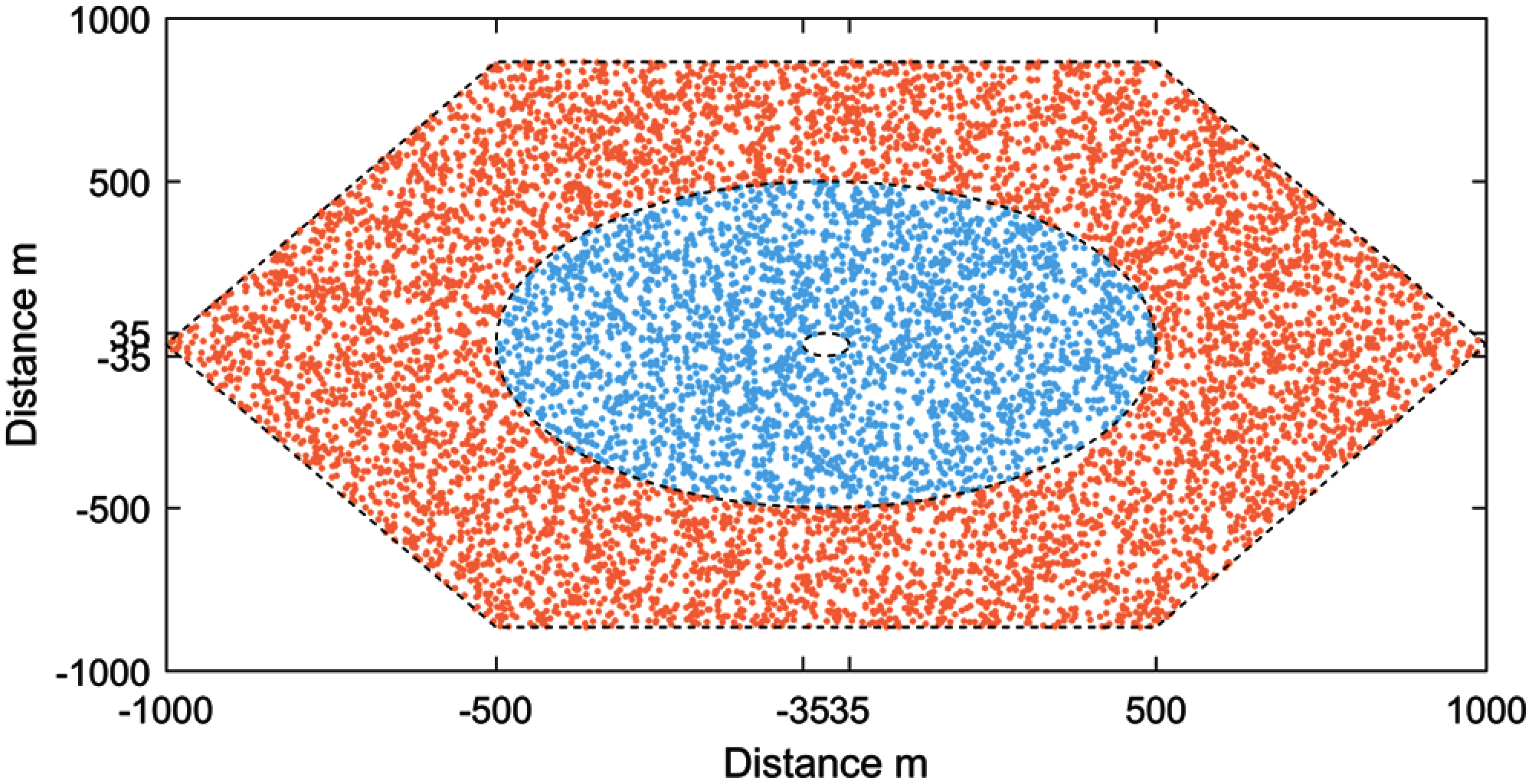
Figure 1: UE distribution in center and boundary coverage areas

Every area is assigned a set of weighting factors γ={γc,γb}, where each weighting factor is a function of time so that it can take different values during the day. The sum of weighting factors at any time instant is always unity i.e., ∑γ=1. Areas of center and boundary areas are:

S={π(rD2−rmin2)33rmax22−πrD2(6)

Network loads vary throughout the day, so in order to capture the daily traffic variation and maximize EE throughout the day, we model each BS as an M/G/m/m state dependent queue [11,13] where M denotes the distribution of the inter-arrival time of users, G the distribution of the service time, m denotes the number of servers, and m denotes the capacity of BS. This queue is also called m-server loss system because number of servers is equal to a maximum number of users, m=Kmax, so there is no waiting lines for additional users, all users after Kmax are blocked. The time of user arrival to BS is independent of that of other users arriving and they arrive according to the exponential distribution with rate λ. BS can serve a maximum number of users simultaneously, M=Kmax, at the peak load, when all Mmax BS antennas are in use. Expected service time is equal to the time for BS i to serve a single user. The service rate is the data rate per user which is dependent on the number of serving users at BS and follows a general distribution G. The change in the number of users at BS will result in the change of the service rate for every user. Thus, if there are n users that are served simultaneously, all of them will have service rate μ(n), but if there is an arrival to BS the service rate will change to μ(n+1). Likewise, if a user is no more served by BS the service rate will change to μ(n−1).

The steady state probabilities for the random number of users n in the BS i are modeled as:

πi(n)=[[λE[T1]]nn!μ(n)μ(n−1)…μ(2)μ(1)]πi(0)πi(0)−1=∑j=om=Kmax{[λE[T1]μ(n)μ(n−1)…μ(2)μ(1)]j1j!}(7)

where πi(0) is the probability that there is no user in cell i, λ is the user arrival rate, E[T1]=dRi(1)is the expected service time when there is a single user in BS, d is the total data traffic contribution by a single user, Ri(1) is data rate when there is a single user in BS i. μ(n)=Ri(n)Ri(1) is the service rate and it is ratio of the data rate of n users in BS, to that of a single user in BS. The data rates for different user states are calculated according to Eq. (2), which is previously defined.

We allow at most 2% blocking at 100% load, i.e., the probability of serving the maximum allowed number of users, m=Kmax simultaneously is 0.02. During our analyses we consider the daily load profile proposed for data traffic in Europe [15]. To find user steady state probabilities at different cell load conditions, we just need to use λt=λmax∗(xt100) where xt is the cell loading at time instant t and λmax can be found using blocking probability πi(Kmax)=0.02. Our objective is to maximize EE by adapting the number of active antennas for any user states.

3  Problem Formulation and Optimization Algorithm

In this paper, we want to maximize the EE of the system described in Section 2. Our EE problem is divided into smaller ones, and the solution to this problem was found through several steps. In order to achieve better EE in the system, it is necessary to adapt the number of active antennas for any user states. This is done iteratively. First, each BS finds the most energy efficient number of active antennas taking into account the interference from the surrounding BSs and a given number of users. This optimal number of antennas Mopt for each user state can be found by maximizing EE for a certain ULD model:

Mopt=argmax:Mi⁡∑k=1Kmax⁡R(k,Mi,)Pitotal(Ki,Mi)subject to Mi≥C1 and Mi≥C2(8)

The constraint C1=PcPmax,PA∗10PAPR comes from the minimum number of antennas by keeping Peak-to-average power ratio (PAPR) of the transmitted signal at 8 dB and the requirement C2=k+1 of ZF precoding. A weighted-average value of Mopt at a certain cell loading condition during time instant t can be calculated as:

Mavgt=[∑k=1Kmax⁡πi(k)∗Mopt(k)](9)

We use the daily load profile proposed for data traffic in Europe however, the mean value can be calculated for another period or part of the day for which we need to have an appropriate load profile for data traffic.

In order to find an optimum number of antennas, we first determine the global optimum point which represents the maximum number of users and antennas within, which we search for the optimal value of the system. Then we formulate the problem to find the optimum cell size, bandwidth, output power level of the BS, and maximum output power of PA. The influence of cell size change on pilot contamination and thus on system performance is analyzed in [25]. Their results show that pilot sequence length significantly increases as the cell radius is reduced, so downlink spectral and energy efficiencies significantly improve. Authors in [26] proved that small cells give high EE, but the EE improvement saturates quickly with the BS density. The potential energy savings that can be achieved through bandwidth expansion at relative low traffic load are investigated in [27].

In order to analyze the performance of our established model with dynamic change of antenna number, a reference model was created which uses a previously determined global maximum number of antennas Mmax. This reference model in our simulations is called a fixed antenna system, because it keeps the Mmax antenna active all the time, regardless of cell changes in terms of the number of active users, cell load, and ULD model, except for the case when there is no user in the system. A significant EE gain was achieved in [28] when specified number of antennas are activated per cell, where the gain in some scenarios was 25%. The gain is the highest when the amount of power allocated to each user is the lowest.

Since changes in the cell are constantly occurring, it is necessary to adapt radio resources to these changes and establish a dynamic allocation of resources that result in high energy efficiency. Authors in [29] proposed two algorithms for EE-oriented resource allocation schemes, which optimize the number of antennas, user selection, and power allocation jointly. The algorithm proposed in [28] firstly shows a low-interference UE grouping algorithm, and then, it presents a resource allocation algorithm based on the results of the user grouping algorithm, which ensure the UEs with better channel quality can be properly allocated on corresponding RBs.

Our algorithm aims to find the optimal number of antennas of BS, taking into account the current state in the cell. But the first step of the algorithm is to find the global optimal number of antennas and users (Mglopt,Kglopt). The determined global optimum of antennas is used to initialize the number of antennas of a fixed system and the initial weighted average optimal number of antennas Mavg. Then, it iteratively updates Miterate with Mavg. For all user states k, we find the vector of antennas that maximizes EE at different user states Mopt(k) using Eq. (8), and we also calculate steady state probabilities πi(k) using Eq. (7). Next, we calculate the weighted average optimal number of antennas, Mavg according to Eq. (9), and adjust Miterate with Mavg until it converges. The search for M that maximizes EE over each user state is step that is computationally the most expensive part in the algorithm, so complexity can be approximated to the order of O(n2).

Similar algorithm was proposed in [10] where authors looking for optimal number of antennas that matches the instantaneous system conditions: cell loading, ULD model, and number of active users. The same conditions are analyzed in our algorithm but ULD model is different. The results match in the part where the ULD model is the same.

The described steps of the proposed strategy are shown in Algorithm 1, and were performed only for one considered cell due to the assumed configuration symmetry in all cells.

4  Results and Discussion

The cellular network in our simulation consists of 19 regular hexagonal cells. BS from each cell transmits a constant output power and the minimum distance from BS is 35 m. The maximum cell radius in the main scenario is 500 m. We distributed 10000 test points in each cell, using the Monte-Carlo insertion method, to calculate average channel variance. Test points are distributed in the area bounded between the circle of minimum cell radius of 35 m and the cell edge according to formed ULD models. Classic wrap-around technique has been applied to avoid edge effects. We assume all cells are symmetrical in BS configuration, ULD, and cell loading variations.

4.1 Impact of the Cell Size on EE

Cell size is a very important factor in the design of massive MIMO networks that can significantly affect system performance and the amount of capital investment which includes infrastructure costs such as base station equipment, backhaul transmission equipment, site installation, and radio network controller equipment. In this scenario, we analyze the impact of cell size on system performance, especially on EE in the two observed coverage areas: center and boundary. We formed three sub-scenarios for three different cell sizes: sub-scenario with a cell radius of 500, 1000, and 2000 m. Users close to the cell boundaries suffer from strong interference, therefore it is important for these users to determine the optimal cell size.

Our results show that EE and Average UR are significantly higher in the CF area than in BF for each considered cell size. But, for all considered scenarios, compared to a system with a fixed number of antennas, both BF and CF users achieve better results when adaptively selecting the number of antennas. Results for EE for all cell size scenarios are shown in Fig. 2.

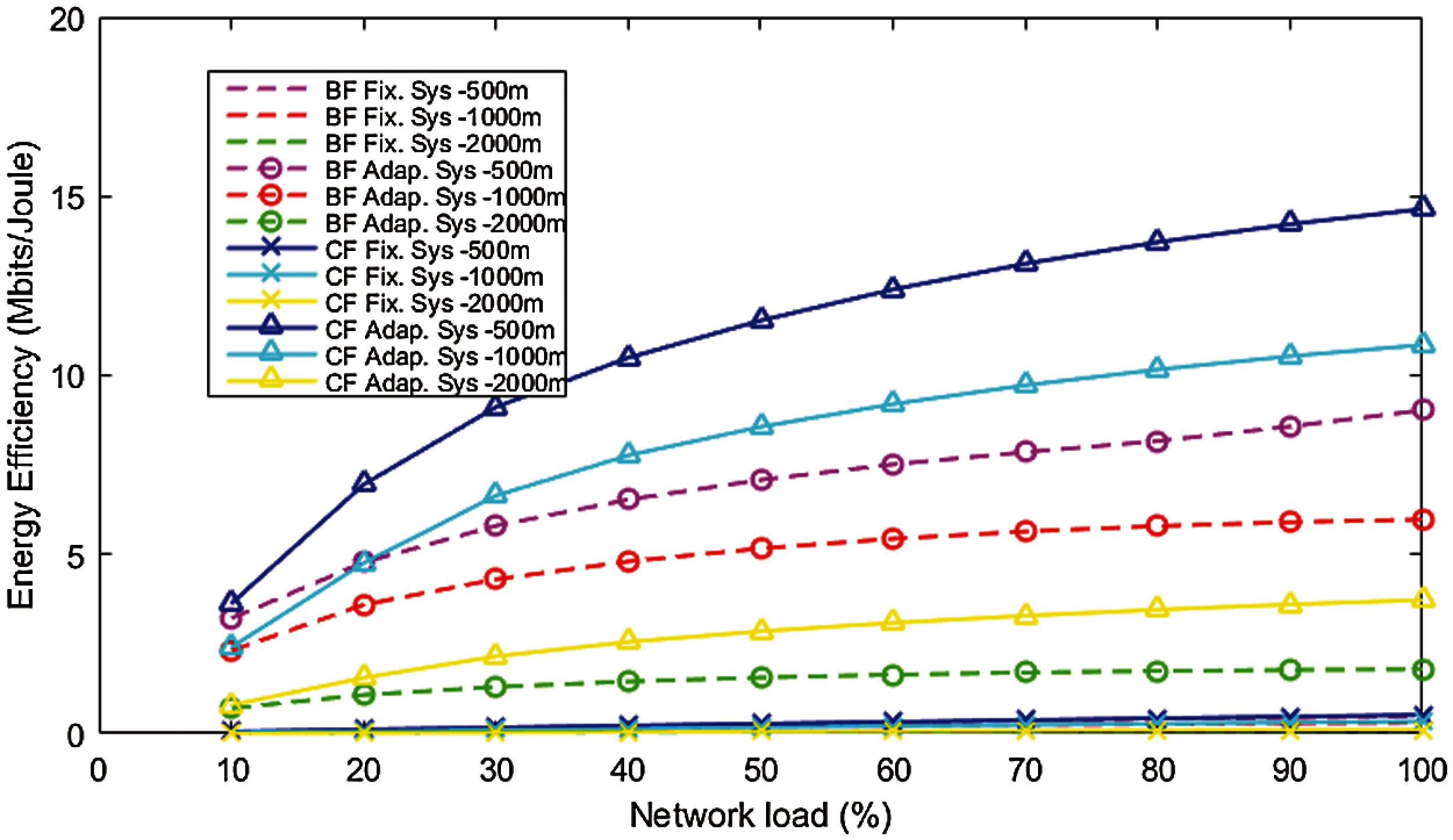
Figure 2: EE as a function of the network load at different cell size and ULD models

Our analysis confirms that EE increases with the cell size shrinking, but reducing the cell size will also decrease the array gain. Therefore, the achievable SE decreases when the cell size is too small. The transmit power decreases with the cell size shrinking because the users will be closer to the BS. Therefore, transmit power is much lower than the circuit power, so EE in the network with a small cell size is dominated by the circuit power. Our results are consistent with findings from [8] where EE also increases with the decrease in cell size and optimum transmit power decrease with the decrease in cell size. Also results in [12] shows that spectral efficiency per user is reduced by the increasing the number of users in the system. This is because resources are distributed among more users. However, in [28] the proposed algorithm achieved an improvement in spectrum efficiency by 28%, when the number of UEs reached 80.

We found that for a cell radius of {500, 1000, 2000} m, the corresponding is {213, 222, 250} and is {100, 97, 91}. Optimal number of antennas for all considered cell sizes when cell load is {10, 50, 100}% and active number of users is {30, 60, 90} are shown in the Tab. 1.

We have also calculated weighted average optimal number of antennas for different cell load and results for cell radius of {500, 1000, 2000} m and cell load {10, 50, 100}% for BF are {38, 132, 213}, {34, 114, 211} and {36, 127, 231}, while for CF results are {31, 65, 120}, {29, 55, 104} and {25, 54, 101}. With the increase of the cell size from 500 to 1000 m, better results of the optimal and weighted average optimal number of antennas were recorded, while a further increase in the cell radius did not result in a decrease in the number of optimal active antennas. With the increase in the active number of users, a larger number of antennas are activated for users from the BF and CF areas, but this activation in the BF area increases significantly with increasing cell load and decreasing cell size so at a cell size of 500 m and a cell load of 100% already at 60 active users BF users require activation of 210 antennas, which is almost the maximum number of antennas (maximum for this case is 213), while CF users for the same number of active users and the same network load require the activation of 132 antennas. The difference between the number of active antennas at different loads decreases with increasing cell size for both BF and CF ULD.

EE gain of our proposed model with adaptive antenna selection has excellent results for both the CF and BF areas and decreases with increasing cell load, but increases with the increase of the cell size. The corresponding EE gain for cell radius of 500 m, and cell load of {10, 50, 100}% for BF is {478.35, 165.44, 92.20}% and for CF is {551.92, 325.70, 201.48}% and is shown on Fig. 3.

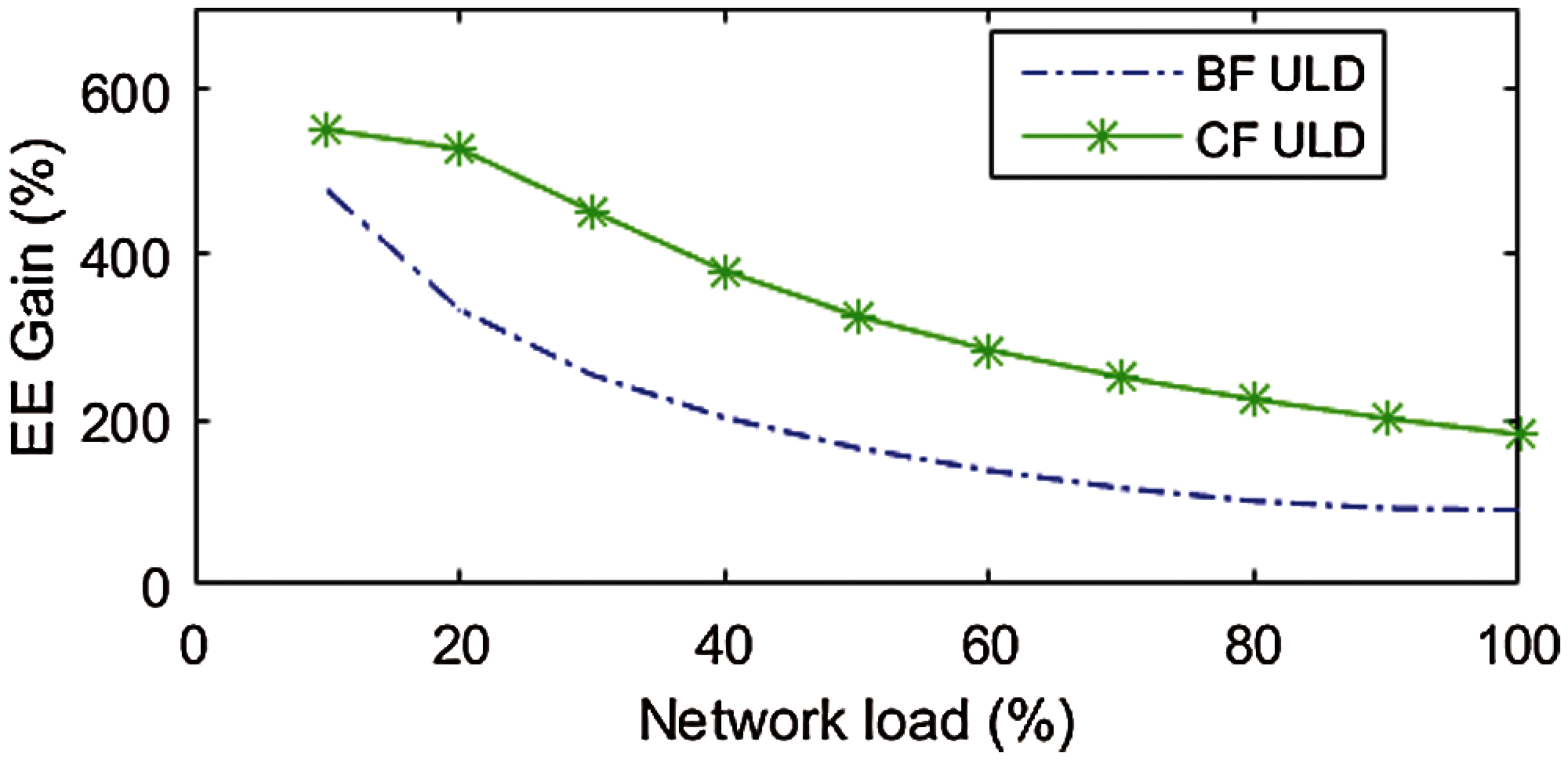
Figure 3: EE gain as a function of the network load for cell size Rmax = 500 m

Also in [10] results have shown that for all ULD models, the obtainable EE gain decreases at different trends as cell loading increases, which is understandable as both systems are in the most energy-efficient state at peak cell load.

It can be concluded that , EE and Average UR increase with the decrease in cell size, while and the difference in EE gain between the proposed adaptive system and the fixed antenna system decrease with the decrease in cell size. From the EE vs. cell radius curve, we get the corresponding optimal cell size is 500 m.

4.2 Impact of the Bandwidth on EE

Since bandwidth is a limited resource, 5G will require the allocation of additional spectrum for mobile broadband and flexible spectrum management capabilities. A set of new frequency bands will be used (licensed, unlicensed, and shared) to supplement the existing wireless frequencies, enabling larger bandwidth operation and substantially improved capacity.

The use of large blocks of spectrum in higher frequency bands and heterogeneous carrier aggregation (particularly above 6 GHz and up to 100 GHz) in addition to unlicensed spectrum have made wider system bandwidths (up to 3.2 GHz) feasible, leading to higher peak data rates and network capacity [30].

This section analyzes the impact of the bandwidth values on the performance of the considered system model. In this analysis, the bandwidth values vary from 20 to 100 MHz in increments of 20 MHz. With the increase in bandwidth, there is an increase in EE and Average UR for CF and BF ULD. In all considered bandwidth scenarios, CF ULD achieved better results than BF ULD, however the difference between the results is not drastic, but with increasing bandwidth and network load, it increases in favor of CF ULD. In all considered scenarios, the proposed adaptive system also achieved better results compared to the fixed one. With the increase in bandwidth, the results of the adaptive system are significantly better. Fig. 4 shows the results achieved for EE as a function of the number of active users in the cell for CF ULD, with different bandwidth values and network load of 20% and 100%.

Figure 4: EE as a function of the number of active users in the cell at different values of bandwidth and network load of 20% and 100% for CF ULD

Despite these improvements, with increasing bandwidth and Mmax are significantly reduced, so for the case of the bandwidth of 100 MHz Mmax=96 and Kmax=43. Therefore, the selection of the appropriate optimal bandwidth depends on the trade-off between the number of users to be served at the same time and the level of desired performance for those users.

4.3 Impact of the Output Power Level of the BS and Maximum Output Power of the PA on EE

This section analyzes the impact of the different output power levels of the BS (Pc–constant for each BS) and maximum output power of the PA (Pmax,PA) on EE in the two observed coverage areas: center and boundary. Four sub-scenarios were created to analyze the impact of both parameters (Pc, andPmax,PA) on EE.

4.3.1 Impact of the Output Power Level of the BS on EE

Values of 10, 20, 30, and 40 W were considered to analyze the impact of the output power level of the BS on EE.

It is very important to analyze how the increase in network load affects the activation of the required number of antennas that ensures a certain output power level of the BS since the increase in the number of active antennas negatively affects the EE. The findings of authors in [11] are the same because they stated that maximal EE depends on the number of antennas that can be selected and in their scenario EE started to decrease when the number of multipath increased at number RF = 100. With the increase in network load, significantly higher antenna activation was observed for the BF ULD compared to CF ULD, but in both cases of ULD, the highest activation was at the output power value of 40 W. The best results, in the case of CF ULD, achieved when the output power level of the BS is 20 W and in this sub-scenario, at maximum network load, it is necessary to activate an average of 60 antennas, whereas in the best sub-scenario for BF ULD which is at Pc=10 W, at maximum network load it is necessary to activate 3 times more antennas on average, i.e., 185 antennas. These sub-scenarios with the lowest average number of active antennas, represent the cases with the best EE, i.e., CF ULD achieves the best EE at Pc=20 W, which is significantly higher than EE in other sub-scenarios. The representation of EE as a function of network load for all considered sub-scenarios with different Pc values is shown in Fig. 5.

Figure 5: EE as a function of the network load at different values of output power level of the BS and ULD models

Based on the obtained results, it can be concluded that the best EE for the case of CF ULD is twice as high as the best achievement of EE in BF ULD. The analyzed sub-scenarios for the BF ULD achieve approximate EE values and there is no drastic increase in EE for a particular sub-scenario when the network load increases.

4.3.2 Impact of the Maximum Output Power of the PA on EE

To analyze the impact of the maximum output power of the PA (Pmax,PA) on EE, four different values for a given parameter were considered: 1, 6, 8, and 16 dB.

Fig. 6 shows the average number of activated antennas for all four sub-scenarios when the network load increases considering the two ULD models created. ULD CF requires the activation of a smaller number of antennas in all considered sub-scenarios with different Pmax,PA, compared to ULD BF.

Figure 6: Average number of antennas as a function of the network load at different values of maximum output power level of the PA and ULD models

For the Pmax,PA=6 dB, ULD CF has activation of the smallest number of antennas, regardless of network load. In this sub-scenario, the average number of activated antennas does not change drastically with increasing load, unlike sub-scenarios with Pmax,PA=8 dB and Pmax,PA=16 dB, when activation increases linearly with network load.

Users in the central area for the 1 dB sub-scenario have a fixed activation of 100 antennas regardless of the network load value because for Pmax,PA=1 dB a delivery of 0.2 W transmit power is achieved. In this case activation of at least 100 antennas is required to maintain a constant output power level of 20 W. Results from [5] also show that when Pmax,PA is low, e.g., 1 dB, the system becomes very efficient at high load but it is not much efficient for the smaller number of users as the number of active antennas cannot be small due to total transmit power constraint.

For the case of ULD BF, the lowest antenna activation is achieved for Pmax,PA=1 dB that is still a higher activation in comparison to all sub-scenarios with different Pmax,PA for CF ULD. In all other sub-scenarios with different Pmax,PA and ULD BF, antenna activation mainly increases linearly with increasing network load but with a sharp increase. For example in the case of Pmax,PA=16 dB and network load of 10% an average of 50 antennas are activated, while for a network load of 100% an average number of activated antenna is equal to the maximum number of antennas of 250.

Fig. 7 shows the impact of the dimensioning Pmax,PA on EE at different network loads for both ULD models.

Figure 7: EE as a function of the network load at different values of maximum output power level of the PA and ULD models

Compared to BF ULD, CF ULD achieved better results for Average UR and EE in all sub-scenarios with different Pmax. At lower network load EE has similar values in all sub-scenarios for both ULD. The sub-scenario with Pmax,PA=6 dB in CF ULD achieves significant EE growth at network load of 30% and with the further increase of network load, which at maximum load almost reaches dimensioning of PA of 1 dB. In the cases of BF ULD, the best result for EE was achieved at 1 dB. Average UR has slightly decreasing values when increasing network load in all sub-scenarios and for both ULDs. The best results for Average UR were achieved with CF ULD for values of 6 and 1 dB, while for BF ULD for the case of the 1 dB.

Based on the results, it can be concluded that as the maximum output power of the PA and the output power level of the BS increases, EE decreases for both ULDs.

4.4 Average Energy Consumption on an Hourly Basis

In addition to the analyzed impact of system parameters on EE for our formed adaptive system model, another important measure of energy consumption and savings that can be achieved during the day by applying the adaptive number of active antennas is average energy consumption per BS expressed in units of kWh:

AEC=∑t=124⁡Ptot(t)∗360024(10)

In this analysis for daily load variation, we use the model proposed for data traffic in Europe [15] like in many others works and the model proposed for business, residential, street, and highway areas [31].

Based on the previous results, the analyzes in this section were performed for an environment with a cell radius of 500 m, a bandwidth of 20 MHz, the output power level of BS is 20 W and the maximum output power of the PA is 6 dB. Also, this analysis was carried out considering the results of our established two areas of coverage (center and boundary) and two new scenarios with the different assignment of weighting factors, S1 and S2. Tab. 2 shows how weighting factors were assigned for the created scenarios S1 and S2.

During daylight hours (8–21 h) S1 has a higher concentration of users in the central area, while during the night hours (22–7 h) higher weighting factors were assigned to users at the edges of the cell. Scenario S2 has the opposite situation with the assignment of weighting factors. Results for CF and BF ULD in all previous scenarios showed that BF ULD performed worse, which is also the case in scenarios S1 during night hours and S2 during daylight hours for all data traffic models, and it is necessary to activate more antennas. However, the system with adaptive antenna activation in all scenarios can turn off a significant number of antennas. Scenario S1 during daylight hours achieves a maximum shutdown of 77 antennas for the model proposed for data traffic in Europe, while Scenario S2 during night hours has a maximum shutdown of 88 antennas in the case of Business data traffic. Results in [10] show conclusively that at least one third of the active antennas can be turned off for half a day for both scenarios with the help of cell load and ULD adaptive antenna system.

Fig. 8 shows the average energy consumption per BS of fixed and adaptive systems in both scenarios and for all analyzed data traffic models.

Figure 8: AEC for fixed and adaptive system and different data traffic models

Compared to the fixed system, the adaptive system achieves significantly lower consumption. In the S1 scenario, a saving of 64% is possible in the Residential model of data traffic, while the maximum saving of average energy consumption in scenario S2 is achieved for the Business data traffic model and is equal to 42%.

5  Conclusion

In this study, we analyzed the energy efficiency of a load adaptive massive MIMO system with two different ULD models. Our results show that the optimal number of antennas depends primarily on ULD model and secondarily on cell loading. We also determined the impact of cell size, available bandwidth, output power lever of the BS, and dimensioning of a power amplifier (PA) at different cell loading on EE. Our developed resource allocation scheme jointly optimizes the number of BS antennas, user load distribution, and cell loading. BF ULD achieved worse results in the analysis of the impact of system parameters on the EE in the fixed and adaptive model of the system and for different network loads. Strong interference from other BSs and weakest signals from its BS are the reasons for poor results in BF ULD, which is why special attention should be paid to users at the edges of the cell when designing the network and establishing algorithms to solve interference. With increasing bandwidth and cell size, the maximum number of simultaneously served users is reduced, which is why the choice of the optimal value for these system parameters depends on the trade-off between the number of simultaneously served users and the level of desired performance for those users. The adaptive system for CF ULD achieves the best EE gains and for cell radius of 500 m, and cell load of {10, 50, 100} their values are {551.92, 325.70, 201.48}%.

During dimensioning the maximum output power of the PA and the output power level of the BS it was concluded that increases in these parameters lead to a decrease in EE. An increase in network load affects the activation of more antennas to ensure a certain output power level of the BS and that number is significantly higher in BF ULD, even in the best sub-scenario (Pc=10 W) BF ULD requires 3 times higher activation compared to the best sub-scenario in CF ULD (Pc=20 W).

Based on the comparison between the performance of fixed and adaptive system model, it was concluded that better results of EE are achieved in the adaptive system for all analyzed scenarios because this proposed system can turn off a significant number of antennas and achieve significantly lower energy consumption. Within the 24 h operation, a savings potential of 64% is achieved in a residential model of data traffic, while saving in other models is in the range of 20–64%.

Funding Statement: The authors received no specific funding for this study.

Conflicts of Interest: The authors declare that they have no conflicts of interest to report regarding the present study.

This work is licensed under a Creative Commons Attribution 4.0 International License, which permits unrestricted use, distribution, and reproduction in any medium, provided the original work is properly cited.