Computers, Materials & Continua DOI:10.32604/cmc.2022.021517
Article

Performance of Gradient-Based Optimizer for Optimum Wind Cube Design

Alaa A. K. Ismaeel1,2, Essam H. Houssein3, Amir Y. Hassan4 and Mokhtar Said5,*

1Faculty of Computer Studies (FCS), Arab Open University (AOU), Muscat, 130, Sultanate of Oman
2Faculty of Science, Minia University, Minia, Egypt
3Faculty of Computers and Information, Minia University, Minia, Egypt
4Electronics Research Institute, Giza, Egypt
5Electrical Engineering Department, Faculty of Engineering, Fayoum University, Fayoum, Egypt
*Corresponding Author: Mokhtar Said. Email: msi01@fayoum.edu.eg
Received: 05 July 2021; Accepted: 15 August 2021

Abstract: Renewable energy is a safe and limitless energy source that can be utilized for heating, cooling, and other purposes. Wind energy is one of the most important renewable energy sources. Power fluctuation of wind turbines occurs due to variation of wind velocity. A wind cube is used to decrease power fluctuation and increase the wind turbine’s power. The optimum design for a wind cube is the main contribution of this work. The decisive design parameters used to optimize the wind cube are its inner and outer radius, the roughness factor, and the height of the wind turbine hub. A Gradient-Based Optimizer (GBO) is used as a new metaheuristic algorithm in this problem. The objective function of this research includes two parts: the first part is to minimize the probability of generated energy loss, and the second is to minimize the cost of the wind turbine and wind cube. The Gradient-Based Optimizer (GBO) is applied to optimize the variables of two wind turbine types and the design of the wind cube. The metrological data of the Red Sea governorate of Egypt is used as a case study for this analysis. Based on the results, the optimum design of a wind cube is achieved, and an improvement in energy produced from the wind turbine with a wind cube will be compared with energy generated without a wind cube. The energy generated from a wind turbine with the optimized cube is more than 20 times that of a wind turbine without a wind cube for all cases studied.

Keywords: Wind turbine; wind cube; gradient-based optimizer; metaheuristics; energy source

1  Introduction

Quality of life improvements are necessary as an economy and society develop. One corresponding challenge is to decrease environmental pollution. Replacing fossil fuels with clean energy is one of the main components to decrease environmental pollution. Renewable energy utilized at a large scale can help to meet daily energy demands [1–5]. Industries and academic institutions alike are interested in developing electricity from renewable and clean energy sources, and with the advancement of existing technology, these factors justify the importance of wind energy in recent years [6,7]. A wind cube is a modern wind turbine built to absorb and amplify more kilowatt-hours (kWh) of wind. When wind hits the wind cube, it concentrates and generates the speed, in turn producing more power. The modern wind cube system has been designed to solve low wind speed problems and collect wind power under these circumstances [8]. Wind cubes are used to improve the efficiency of wind turbines and result in great productivity [8]. Because of the wind's nonlinear nature, optimization techniques are essential. Optimizing the layout is achieved through soft computing technology [7]. The meta-heuristic optimization algorithms are used to extract the optimum solution for several problems. One of these problems is the estimation of parameters in photovoltaic models such as the Harris Hawks optimization [9], the Marine Predators Algorithm [10], the multi-strategy success-history-based adaptive differential evolution [11], the bacterial foraging algorithm [12], the differential evolution algorithms [13], Enhanced leader particle swarm optimization (ELPSO) [14], Time varying acceleration coefficients particle swarm optimization (TVACPSO) [15], and the shuffled frog leaping algorithm [16]. Meta-heuristic optimization applied to a wind farm layout is one of the main tools used to determine optimum wind farm position and maximize the generated power. The optimization algorithms used for these are modified genetic algorithms based on a Boolean code [17], the Monte Carlo method [18], a genetic algorithm-based local search [19], a new pseudo-random number generation method [20], and a multi-level extended pattern search algorithm [21].

The following items summarize the contributions of this paper:

•   Increasing the power generated from the wind turbine over a year using the wind cube.

•   The inner and outer radius of the wind cube, roughness factor and the height of the wind turbine hub are the decision variables extracted using a new optimization algorithm (Gradient-Based Optimizer).

•   Comparison between the proposed GBO algorithm with Tunicate swarm algorithm (TSA) and Chimp optimization algorithm (ChOA) is performed for the same wind turbine.

•   Minimizing the probability generated energy loss.

•   Minimizing the wind turbine and wind cube cost using the meter cubic function.

•   Comparison between the power generated from the wind turbine with and without a wind cube.

The paper organization is as follows, Section two explains the problem formulation and metrological data. The objective function is illustrated also in Section 2. Section 3 dissects the Gradient-Based Optimizer algorithm. The study cases are illustrated in Section 4. The conclusion and future work is in Section 5.

2  Problem Formulation and Metrological Data

2.1 Wind Turbine Analysis

The variation of wind speed is the main factor affecting the power generated from the wind turbine. The characteristics of wind turbine output power are dependent on the boundaries of the wind speed (cut-in speed Vci, rated speed Vr and cut-off speed Vco) as in the following equation [22,23]:

Pwind={Pr(V3−Vci3Vr3−Vci3)Vci≤V≤VrPrVr≤V≤Vco0Vco≤VorV≤Vci (1)

where Pr and Vr are the rated power and rated speed, respectively. The hub height of the wind turbine is affected by the stream speed to the wind turbine, so that the stream velocity is changed according to the hub height with the following equation [24]:

Vh.2Vh.1=(h2h1)∝ (2)

where Vh.2 is the velocity at the new hub height h2 and Vh.1 is the reference velocity at the reference hub of height for the wind turbine h1. For the neutral stability condition, α is the roughness ingredient factor which ranges from 0.14 to 0.25 [25]. The improvement of the power generated from the wind turbine is processed using the wind cube. The principle theory for wind cube design is the Bernoulli theory. The wind cube size is changed to achieve the optimal design. The configuration of the wind cube is explained in Fig. 1.

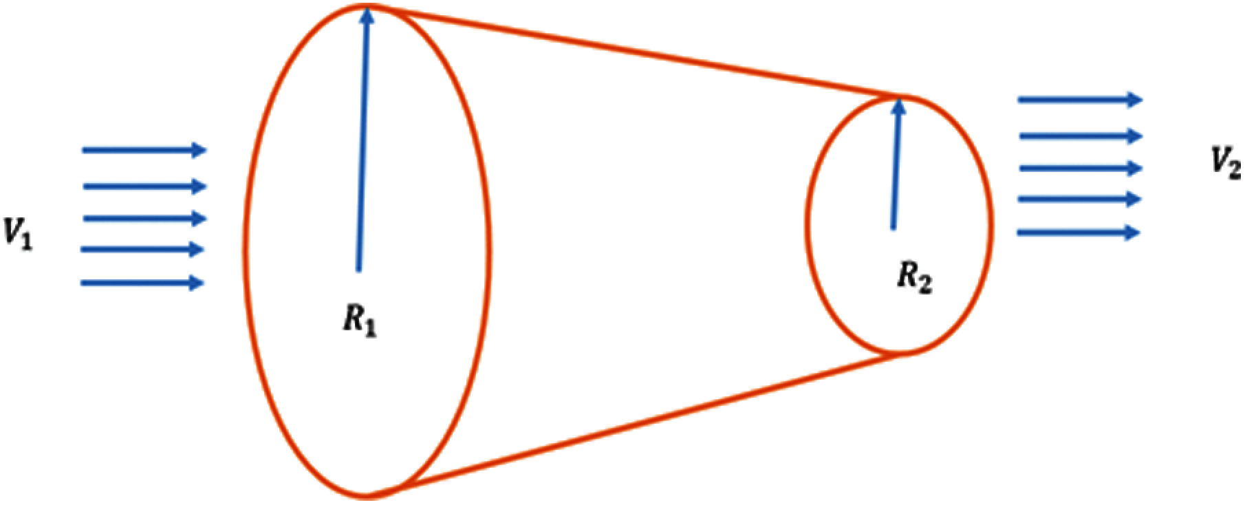
Figure 1: Wind cube configuration

Based on Bernoulli’s theory and continuity equation, the main equation for the wind cube is shown as follows:

A1V1=A2V2 (3)

where V1 is the wind speed input to the wind cube from the air side, V2 is the wind speed output from the wind cube, A1 is the area of the wind cube from the air side and A2 is the area of the wind cube from the wind turbine side. The power generated from the wind turbine with the wind cube is given in this equation:

Pwind={ Pr((R12V1R22)3−Vci3Vr3−Vci3)Vci≤V1≤VrPrVr≤V1≤Vco0 Vco≤V1orV1≤Vci (4)

where R1 is the input radius of the wind cube from the air side and R2 is the output radius of the wind cube from the wind turbine side.

2.2 Metrological Data

Hurghada City in the Red Sea governate of Egypt is the site used in this work to simulate the power output improvement. The latitude is 27∘15′26.57"N and the longitude is 33∘48′46.48"E. The metrological data of the average wind speed for each month is explained in Fig. 21., and the average wind speed over the year is shown in Fig. 31.

2.3 Analysis of Objective Function

The improvement to the power generated from the wind turbine corresponds with decreasing the loss of energy generated probability (LEGP) with the maximum speed out from the outer radius of the wind cube not increasing 80% of the cut-off speed for the turbine. The decision variables required for optimal sizing are the two radiuses of the wind cube, the wind turbine hub’s height, and the roughness factor. The mathematical equation for the LEGP is as follows:

LEGP=Eg.rated−Eg.actualEg.rated (5)

where Eg.rated, is the energy generated at rated power from the wind turbine, Eg.rated. The proposed algorithm is applied to an independent run for the objective function before another objective function (meter cubic function) is applied to choose the optimal solution that achieves the minimum parameters. The minimum parameters indicate that the cost of the wind turbine and wind cube is at its minimum. The second objective function is as follows:

fobj2=R1×R1×h2 (6)

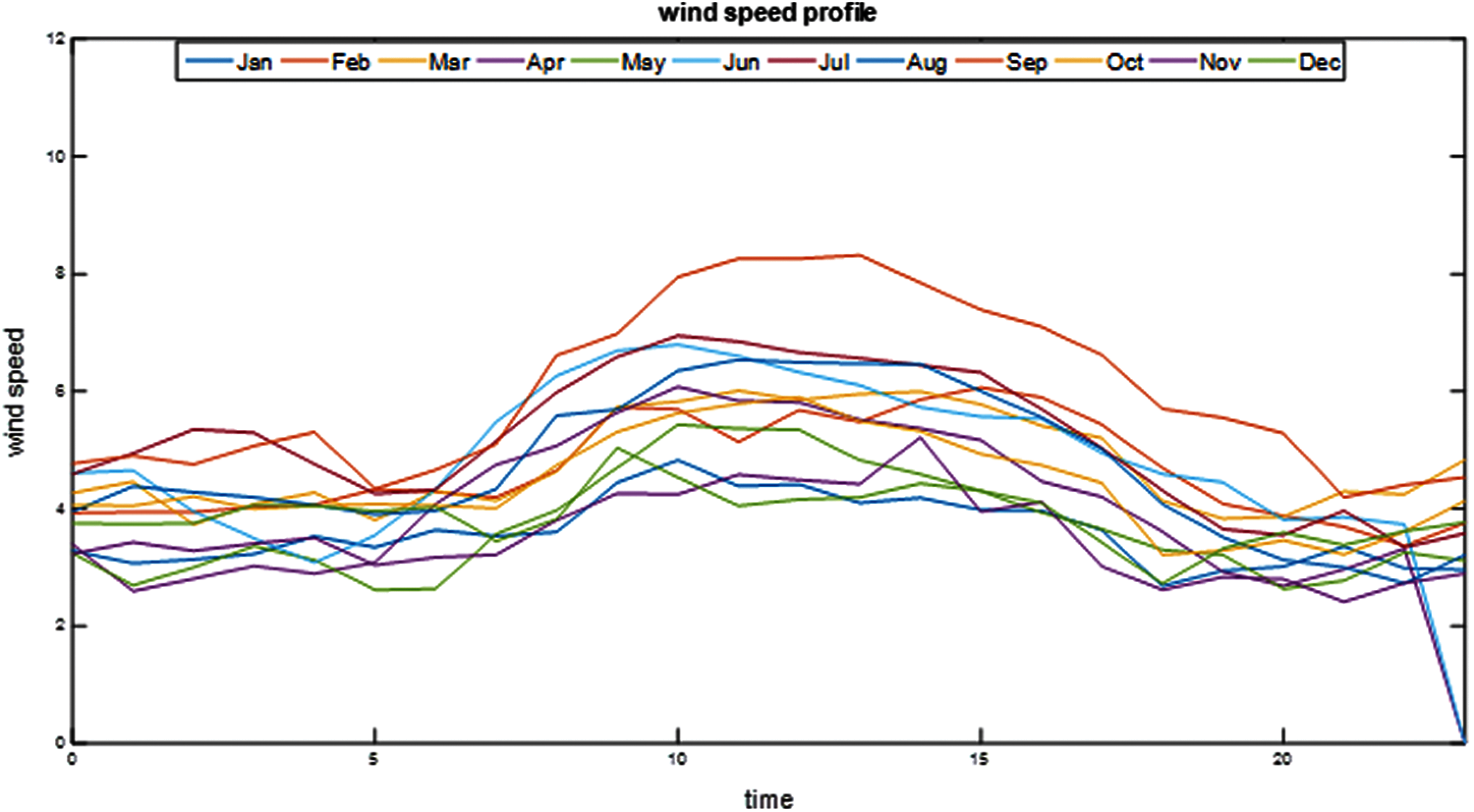
Figure 2: The average wind speed for each month

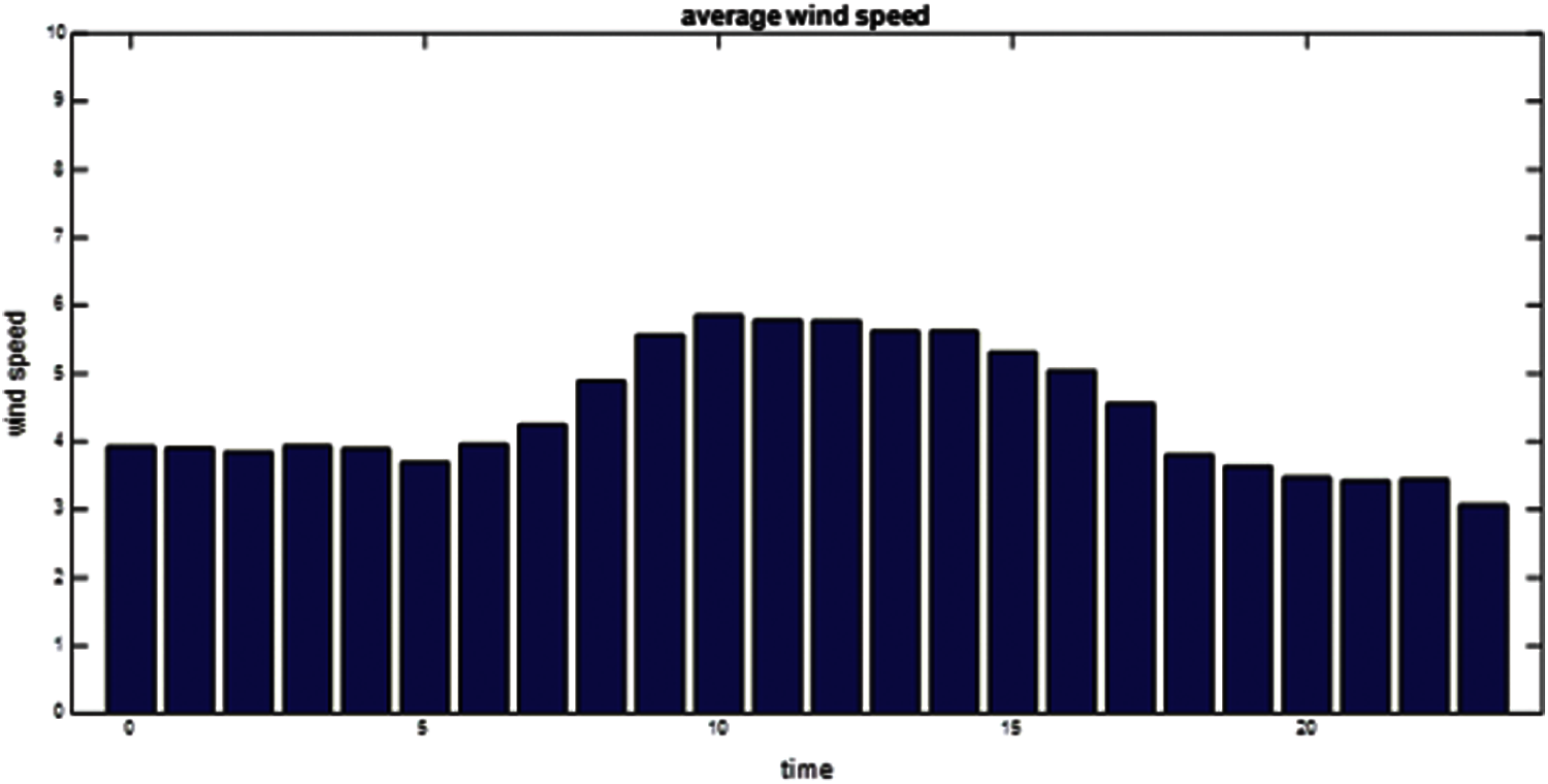
Figure 3: The wind speed average over the year

3  Gradient-Based Optimizer (GBO)

Recently, Ahmadianfar et al. [26–28] have proposed a new metaheuristic algorithm called the Gradient-Based Optimizer (GBO), which mimics the gradient and population-based methods together. In the GBO, in order to explore the search domain utilizing a set of vectors and two main operators (like local escaping operators and the gradient search rule), Newton’s method is utilized to specify the search direction. The main process of the GBO are as follows:

3.1 The Initialization Process

In the GBO, the control parameters α and the probability rate are used to balance and switch from exploration to exploitation. Furthermore, the population size and iteration numbers are due to the problem’s complexity. In the GBO, N vectors in a D-dimensional search space can be defined as:

Xn,d=[Xn,d,Xn,d,…Xn,d],n=1,2,…N;d=1,2,… (7)

Usually, the initial vectors of the GBO are randomly generated in the D-dimensional search domain, which can be defined as:

Xn=Xmin+rand(0,1)×(Xmax−Xmin) (8)

where Xmin, and Xmax are the bounds of decision variables X, and rand(0,1) is a random number in [0, 1].

3.2 Gradient Search Rule (GSR) Process

In the GBO algorithm, to guarantee a balance between exploration of significant search space regions and exploitation to reach near optimum and global points, a significant factor ρ1 is employed as follows:

ρ1=2×rand×α−α (9)

α=|βsin(3π2+sin(β×3π2))| (10)

β=βmin+(βmax−βmin)×(1−(mM)3)2 (11)

where βmin and βmaxare constant values 0.2 and 1.2, respectively, m represents the current iteration number, while M represents the total number of iterations. Particularly, the parameter ρ1 is responsible for balancing the exploration and exploitation based on sine function α. This parameter value changes through iterations, starting with a large value through first the optimization iterations to improve population diversity. Then the value decreases through iterations to accelerate population convergence. The parameter value increases through defined iterations within a range [550, 750] to increase solution diversity and convergence around the best obtained solution. This also allows for exploration of more solutions, therefore enabling the algorithm to avoid local sub-regions. Thus, GSR can be determined as follows:

GSR=randn×ρ1×2Δx×xnxworst−xbest+ε (12)

The concept of GSR is to provide the GBO algorithm with a random behavior through iterations, therefore strengthening exploration behavior and escape from local optima. In Eq. (12), it is defined by the factor Δx that delivers the difference between the best solution xbest and a randomly selected solution xr1m. The parameter δ is changed through iterations due to Eq. (15). In addition, a random number randn is included to improve exploration as follows:

Δx=rand(1:N)×|step| (13)

step =(xbest−xr1m)+δ2 (14)

δ=2×rand×(|xr1m+xr2m+xr3m+xr4m|4−xnm) (15)

where rand(1:N) is a vector of N random values ∈[0,1]. Also, four random integers are chosen from [1, N] which are r1–r4 such that r1≠r2≠r3≠r4≠n, and the parameter step represents a step size which is determined by xbest and xr1m.

Moreover, Direction Movement (DM) is employed to converge around the solution area xn. To provide a convenient local search tendency with a significant effect on the GBO convergence, the term DM uses the best vector and moves the current vector xn in the direction of xbest − xn and is computed as follows:

DM=rand×ρ2×(xbest−xn) (16)

where, rand is a uniform distributed number within the range [0, 1], and ρ2 is a random parameter employed to modify step size of each vector agent. The ρ2 parameter is considered a significant parameter of the GBO exploration process. The ρ2 parameter is computed as follows:

ρ2=2×rand×α−α (17)

Finally, depending on these terms GSR and DM, Eqs. (18) and (19) are used to update the position of the current vector xnm.

X1nm=xnm−GSR+DM (18)

where, X1nm is the new vector generated by updating xnm. According to Eqs. (12) and (16), X1nm can be reformulated as:

X1nm=xnm−randn×ρ1×2Δx×xnxworst−xbest+ε+rand×ρ2×(xbest−xn) (19)

where ypnm and yqnm are equal to yn+Δx and yn−Δx, respectively, and yn is a vector equal to the average of the two vectors: current solution xn and the vector zn+1 that are calculated as follows:

zn+1=xn−randn×2Δx×xnxworst−xbest+ε (20)

while xn represents the current solution vector, randn is a random solution vector of dimension n, xworst and xbest represent the worst and best solutions, and ∆x is given by Eq. (13). Based on the previous formula, when replacing the best solution vector xbest with the current solution vector xnm, we get X2nm as follows:

X2nm=xbest−randn×ρ1×2Δx×xnmxworst−xbest+ε+rand×ρ2×(xr1m−xr2m) (21)

Specifically, the GBO algorithm aims to enhance the exploration and exploitation phases using Eq. (19) to improve the global search for the exploration phase, while Eq. (21) is used to improve the local search capability for the exploitation phase. Finally, the new solution for the next iteration is as follows:

xnm+1=ra×(rb×X1nm+(1−rb)×X2nm)+(1−rα)×X3nm (22)

where ra, and rb are random numbers determined in the range [0, 1], and X3nm is defined as:

X3nm=Xnm+1−ρ1×(X2nm−X1nm) (23)

3.3 The Local Escaping Operator (LEO) Process

The LEO is introduced to strengthen the performance of the optimization algorithm to solve complex problems. The LEO can effectively update the position of the solution, to assist an algorithm to exit local optima points and speed the convergence of the optimization algorithm. The LEO targets generate a new solution with a superior performance XLEOm by several solutions (Xbest best solution, the solutions X1nm and X2nm are randomly selected from population, Xr1m, X1r2m are randomly generated solutions) to update the current solution effectively. This process is performed based on following scheme:

XLEOm={Xnm+1+f1(u1xbest−u2xkm)+f2ρ1(u3(X2nm−X1nm)+u2(xr1m−xr2m))/2,if rand<0.5xbest+f1(u1xbest−u2xkm)+f2ρ1(u3(X2nm−X1nm)+u2(xr1m−xr2m))/2,otherwise (24)

where pr is a probability value, pr = 0.5, the values f1 and f2 are uniform distribution random numbers ∈[−1,1], and u1, u2 and u3 are random values generated as follows:

u1={2×rand,if μ1<0.51,otherwise (25)

u2={2×rand,if μ1<0.51,otherwise (26)

u3={rand,if μ1<0.51,otherwise (27)

where rand represents a random number ∈[0,1] and μ1 is a number in range [0,1]. The previous equations for u1, u2 and u3 can be simply explained as follows:

u1=L1×2×rand+(1−L1) (28)

u2=L1×rand+(1−L1) (29)

u3=L1×rand+(1−L1) (30)

where L1 is a binary parameter take value 0 or 1, such as if parameter μ1<0.5, then value of L1=1, otherwise L1=0. Where the solution xkm is generated as follows:

xkm={xrand,if μ2<0.5xpm,otherwise (31)

where xrand is a random generated solution according to the following formula:

xrand=Xmin×rand(0,1)×(Xmax−Xmin) (32)

and xpm is a randomly selected solution from the population, μ2 is a random number ∈[0,1]. For more details about GBO see [24].

4  Analysis of Results and Discussion

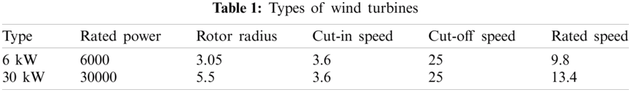
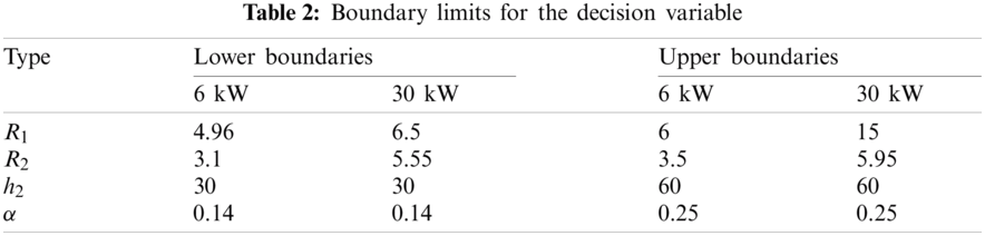
For fair benchmark comparison, the simulation settings are the same for all algorithms. furthermore, the algorithm parameter is set to their default values. This section presents the analysis of the proposed algorithm's results for the wind turbine explained in Tab. 1. The boundary limits for the decision variable of each turbine are explained in Tab. 2. The selection of boundaries for each turbine is dependent on the rotor blades radius and the height of the turbine hub. The wind cube radius from the turbine side is not almost less than the rotor blades radius. The wind cube radius from the airside is more than the rotor blade radius and smaller than the hub height with a specific distance according to each turbine to ensure that the cube does not touch the ground.2,3

4.1 Wind Turbine of 6 kW

Based on analysis described in Section 2 and data reported in Tabs. 1 and 2, the proposed GBO algorithm is applied to the 6-kW wind turbine. Tab. 3 explains the proposed GBO algorithm’s results for a 6-kW wind turbine based on minimizing the loss of the probability of a generated energy loss. The optimum solution for these results is determined according to the second objective function that satisfies the minimum meter cubic function.

Tab. 3 shows that all runs achieve zero probability of generated energy loss; the result in run 30 is the optimum solution due to this solution achieving the minimum objective function of minimizing the meter cubic function. Tab. 4 show the best solution from the proposed GBO algorithm in compared with Tunicate swarm algorithm (TSA) [29] and Chimp optimization algorithm (ChOA) [30] for 6-kW wind turbine. Based on this results the proposed GBO achieve the best meter cubic function compared with the other competitor algorithms. Fig. 4 shows the power demand output from the wind turbine without a wind cube at the same height as the wind turbine hub and the optimum solution's roughness coefficient. Fig. 5 shows the power demand output from the wind turbine with wind cube at the optimum solution for run 30 of the proposed GBO algorithm.

4.2 Wind Turbine of 30 kW

Based on analysis described in Section 2 and data reported in Tabs. 1 and 2, the proposed GBO algorithm is applied to the 30-kW wind turbine. Tab. 5 explains the proposed GBO algorithm’s results for a 30-kW wind turbine based on minimizing the loss of the probability of a generated energy loss. The optimum solution for these results is determined according to the second objective function that satisfies the minimum meter cubic function.

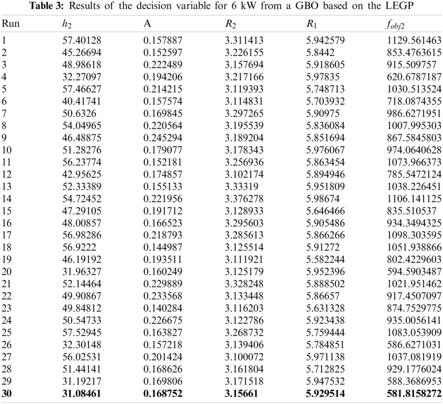
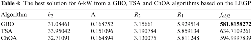
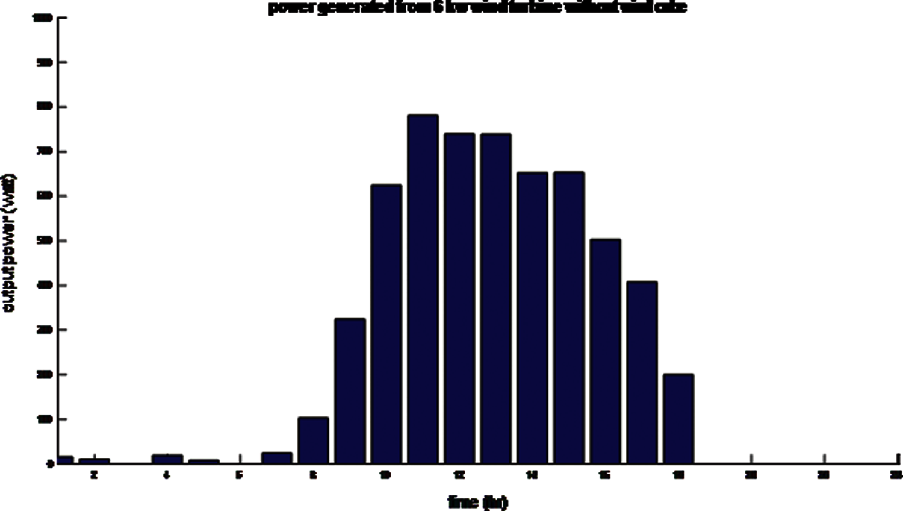
Figure 4: Power generated from a 6-kW wind turbine without a wind cube

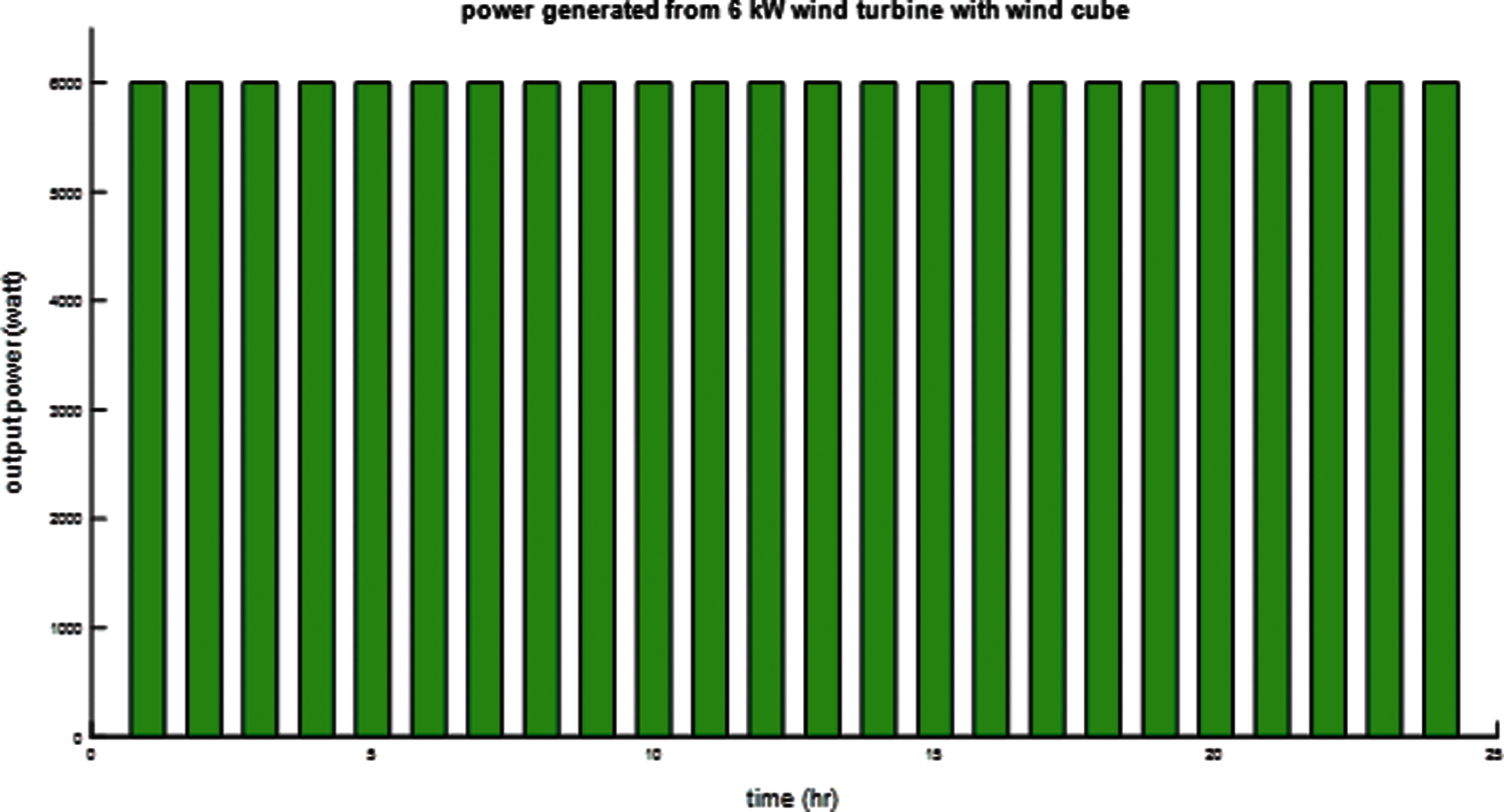
Figure 5: Output power of a 6-kW wind turbine with an optimized wind cube

Tab. 5 shows that all runs achieve 0.079240007 probability of a generated energy loss; the result in run 23 is the optimum solution because this solution achieves the minimum objective function of minimizing the meter cubic function. Tab. 6 show the best solution from the proposed GBO algorithm in compared with Tunicate swarm algorithm (TSA) and Chimp optimization algorithm (ChOA) for 30-kW wind turbine. Based on this results the proposed GBO achieve the best meter cubic function compared with the other competitor algorithms. Fig. 6 shows the power demand output from the wind turbine without a wind cube at the same height as the wind turbine hub and the optimum solution's roughness coefficient. Fig. 7 shows the power demand output from the wind turbine with a wind cube at the optimum solution for run 30 of the proposed GBO algorithm.

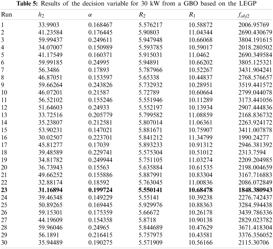
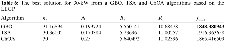
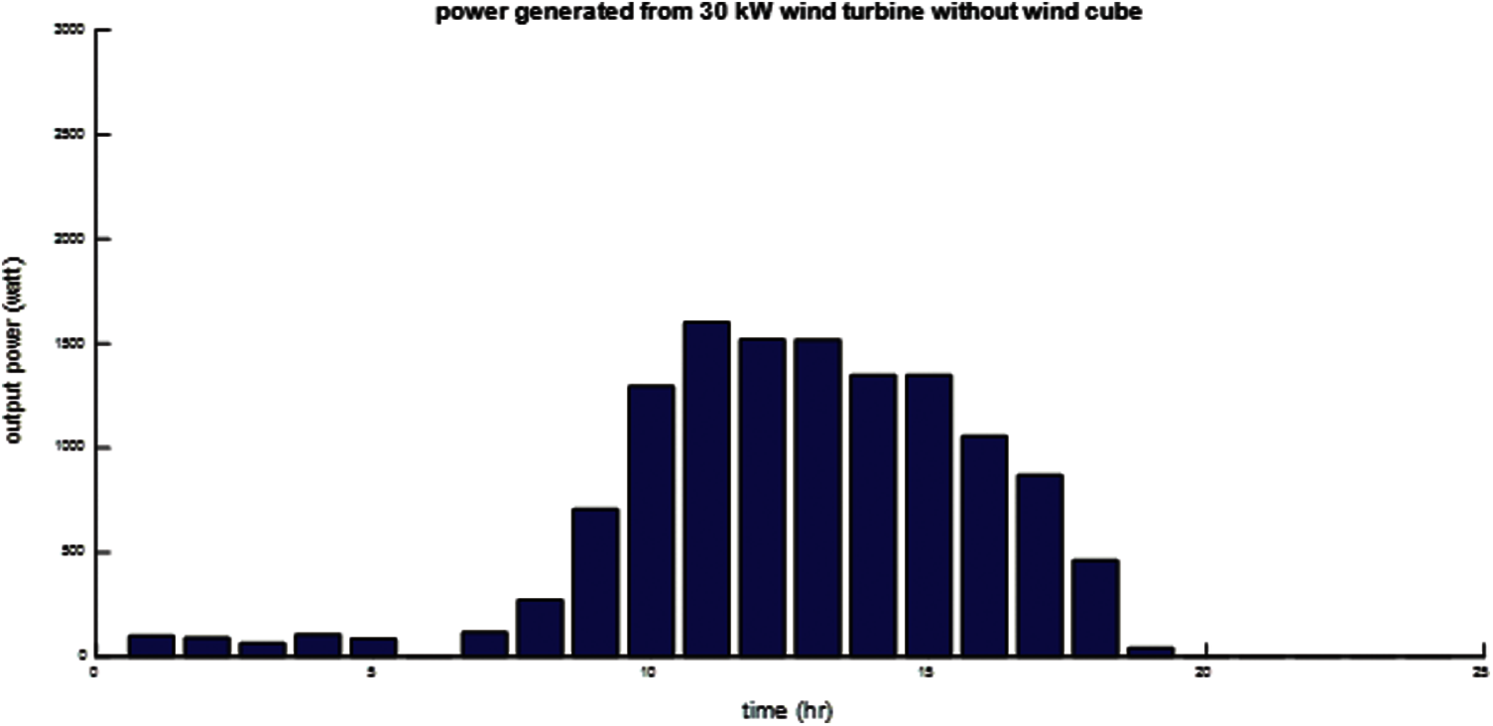
Figure 6: Power generated from 30-kW wind turbine without a wind cube

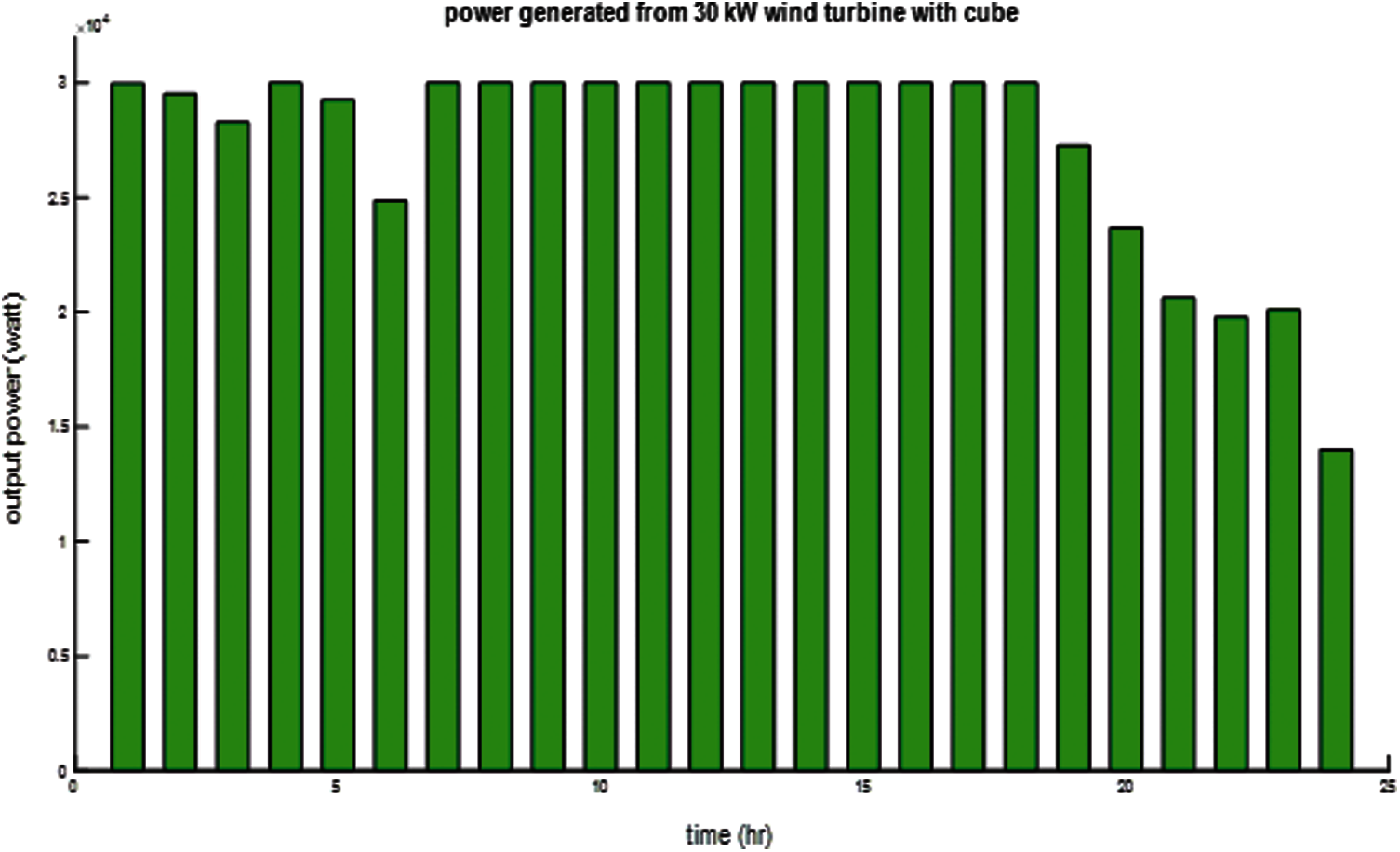
Figure 7: Output power of a 30-kW wind turbine with the optimized wind cube

5  Conclusion

Increasing the generated energy from the wind turbine is important work. Wind cubes improve wind turbine output using an effective optimization technique. A GBO is used to estimate the roughness factor’s decision variable, the inner radius of the wind cube, the wind turbine hub's height, and the outer radius of the wind cube. The extraction of these parameters is dependent on minimizing the probability of a loss of generated energy and decreasing the decision variable to make these variables more cost-efficient. There is a tolerance of a 20% air speed increase for the site as compared with the speed recorded in this work. A comparison between wind turbine output power with and without the optimized wind cube was performed. Based on this comparison, the energy generated from a 30-kW wind turbine with the optimized wind cube as 55.7317 times the energy generated without the wind cube. The energy generated from a 6-kW wind turbine with the optimized wind cube is 23.8123 times the energy generated without the wind cube. The future work will concentrate on apply GBO for several problems such as power flow in power system, wind farm layout problem.

Funding Statement: The authors received no specific funding for this study.

Conflicts of Interest: The authors declare that they have no conflicts of interest to report regarding the present study.

1http://www.wunderground.com

2https://en.wind-turbine-models.com/turbines/493-aeolian-aeo-20

3https://en.wind-turbine-models.com/turbines/1380-aerolite-a-11

This work is licensed under a Creative Commons Attribution 4.0 International License, which permits unrestricted use, distribution, and reproduction in any medium, provided the original work is properly cited.