Computers, Materials & Continua DOI:10.32604/cmc.2022.021642
Article

Decoding of Factorial Experimental Design Models Implemented in Production Process

Borislav Savkovic1, Pavel Kovac1, Branislav Dudic2,3,* and Michal Gregus2

1University of Novi Sad, Faculty of Technical Sciences, Novi Sad 21000, Serbia
2Comenius University in Bratislava, Faculty of Management, Bratislava, 820054 Slovakia
3University Business Academy, Faculty of Economics and Engineering Management, Novi Sad 21000, Serbia
*Corresponding Author: Branislav Dudic. Email: branislav.dudic@fm.uniba.sk
Received: 09 June 2021; Accepted: 07 September 2021

Abstract: The paper deals with factorial experimental design models decoding. For the ease of calculation of the experimental mathematical models, it is convenient first to code the independent variables. When selecting independent variables, it is necessary to take into account the range covered by each. A wide range of choices of different variables is presented in this paper. After calculating the regression model, its variables must be returned to their original values for the model to be easy recognized and represented. In the paper, the procedures of simple first order models, with interactions and with second order models, are presented, which could be a very complicated process. Models without and with the mutual influence of independent variables differ. The encoding and decoding procedure on a model with two independent first-order parameters is presented in details. Also, the procedure of model decoding is presented in the experimental surface roughness parameters models’ determination, in the face milling machining process, using the first and second order model central compositional experimental design. The simple calculation procedure is recommended in the case study. Also, a large number of examples using mathematical models obtained on the basis of the presented methodology are presented throughout the paper.

Keywords: Mathematical modeling; design of experiments; functions; coding; decoding; variable; regression coefficients

1  Introduction

The model expresses the essential properties of an object, process or system. The mathematical model itself consists of a system of equations, states and algorithmic rules [1,2]. This includes the appropriate algebraic techniques used in considering exact solutions in equations [3]. When setting up a mathematical model, basic sources of information are used.

The main goal of mathematical modeling is:

•   calculation and analysis of the object, process or system in order to obtain new and more complete knowledge and legality of the studied process;

•   discovering the mechanisms of interaction within the studied process;

•   testing the set hypotheses about the rightness mechanisms of internal interactions and systems;

•   forecasting the state and behaviour of processes, systems and phenomena;

•   optimization based on set optimization criteria;

•   management of objects, processes or systems in space and time [4].

The field of application of mathematical modeling is very widespread and wide. There are some important mathematical models that are used to explain the computational properties of real world problems and they have been described in the literature, such as [5,6]. Fractional derivatives with a non-distinct nucleus as well as nonlinear crystal shapes were processed by mathematical models. The application of complex dynamic tools in order to solve nonlinear equations is a growing area of research in literary works [5,7]. Thus, in the literature we find the application of factor plans in complex systems that deal with the distribution of supply of appropriate products to different locations by different suppliers and levels of quality of raw materials [8]. As well as specific activities, such as the implementation of digital marketing with the analysis of influencing factors on its profitability in relation to the already existing traditional print marketing [9]. Furthermore, it is also possible to apply factor plans in determining the investments of individual companies in developing countries, all in relation to the factors that affect the level and amount of these investments. This refers, for example, to factors such as the level of education of the population in the regions where an industrial giant wants to be implemented, the age of the population, the amount of payroll taxes, the inflow of foreign direct investment, investment in infrastructure projects [10]. All these factors can be described mathematically using the language of numbers. That such models are not only applicable in the field of economics is shown by other areas of application. Thus, we find application in the transport sector in order to present a mathematical model for the transition of the traffic signal plan [11]. A mathematical model for predicting the reduction of wüstite crystals during the casting process has also been developed [12]. Also in the literature we find the application of the factor plan for determining the optimal level of carbon adsorption in order to remove dyes from aqueous solutions [13]. We find a very interesting work from the aspect of the complexity of influencing factors in the research of “elegance” as a characteristic of a good system [14]. The authors analyze elegance in the context of systems engineering from the aspect of eight different factors, among which the visual arts, Gestalt psychology, neuroscience and complexity theory stand out.

Finally, when observing the application of the factor plan in production systems, the range is endless. Thus, we find application in the field of metallurgical characteristics such as identification of corrosion intensity [15], optimization of tool trajectory in order to increase productivity [16], selection of the most favourable tool angles from the aspect of precision [17], determining the measurement uncertainty of the coordinate measuring machine [18], selection of the most favourable processing regimes from the aspect of machinability [19–23], determining the state of construction systems, in terms of damage [24], testing the influence of operating parameters on the rotating elements of the machine [25].

Application of the design of experiments (DoE) in illustration or in the analysis of results is very common. The field of application is wide, and this can also be seen through the literature sources [26–29] where different spheres of scientific research are represented. Thus, we find the application of DOE in testing the physical and mechanical properties of resins used as organic coatings [22]. DOE application can be found in the optimization of yields of appropriate agricultural crops, where the effects of individual concentrations of appropriate media such as yeast are examined [23]. DOE also finds its wide application in the production of glass fibers [24], as well as in the examination of light effects in photocatalysts [25].

Also, it can be stated that the equations obtained on the basis of DoE can serve as a basis for the application of modeling through artificial intelligence. Thus, we have examples that the limit values in modeling with the help of genetic algorithms are determined on the basis of already existing values in the equations, which were previously obtained on the basis of DoE [19,30–32]. The authors in the paper [26] on the basis of regression values obtained on the basis of DOE analysis form a model for the prediction of tool life. When optimizing the processing parameters of difficult-to-process composite pipes in the form of finding the optimal cutting force, genetic algorithms were applied, which based their regression coefficients on models obtained with the help of DOE [27]. When testing the properties of gasoline engines, DOE was used as a basis on which, through genetic algorithms, expansion to non-orthogonal spaces was performed, which is a common problem in engineering applications [28].

Based on the literature review, it can be stated that the basic characteristics of multifactor experimental plans are the minimum set of experimental points within the experimental hyperspace (many times lower costs and shorter duration of expensive experimental tests), as well as the maximum set of information on the effects of the mathematical model of the process formed thanks to the research according to the cybernetic approach.

The first stage of experimental research is the collection, study and analysis of all available and relevant information about the object of research. The results of the first stage are: a list of influencing factors (preferably ranked according to the degree of influence), the scattering limit and other characteristics of the factors, criteria and optimization parameters in accordance with the set goal and the like. If the number of influential factors is large, it is necessary to separate a smaller number of significant ones from a larger number of less influential ones, by applying appropriate methods.

In key works from the theory of engineering experiment [33–36] the decoding of mathematical models is avoided, already the model is left in coded coordinates and the actual values are obtained by logarithm zing the calculated values. In that way, deviations from the actual values occur.

Specifically, this paper deals with the coding and decoding of factorial experimental design models. The procedures for selecting and defining the range or rank of each independent variable are presented. The possibility of choosing the most favorable mathematical model from the aspect of various researches is given in order to obtain the simplest or most accurate model.

2  Selection and Coding of Model Parameters

The experimental space is determined by possible values of independently variable quantities xij. In this area there are all the points of the experimental plan, which correspond to the regimes and conditions for the test.

The most common multifactor models are experiments in which the factors vary in two levels (maximum and minimum value), where the mean value of the factor is not treated as a level of variation. These are experiments of the type:

N=2k+n0,(1)

where: k-number of factors (variables), n0–number of experimental variables.

The matrix plan of a multifactor plan must satisfy the conditions of symmetry, normality and orthogonality. The orthogonality of the plan is one very important feature of the experimental plan. Mathematically defined:

∑xiuxju=0,i≠j,i,j=0,1,2,…,k.(2)

This characteristic of the plan means that the information matrix and the dispersion matrix are transformed into a diagonal one. This means that the regression coefficients are calculated (evaluated) independently of each other. This greatly simplifies the calculation of these coefficients.

The rotatability of the centrally composite plan of the experiment is achieved by adding the state of the experiment so that all states are equally distant from the center of the experiment, i.e., rotatability depends on the axial distance α (distance of the state in the axes from the center).

Special selection of parameters xij (3) simplifies solving the system of equations for determining the regression coefficients by reducing the coefficient matrix to the unit matrix.

If the level and size xij are encoded using the transformation Eq. (4), then the change in size will be determined by the interval:

−1≤xi≥+1,i=1⋯k.(3)

The coded start is moved from the original point to a new point, which indicates the zero level of the factor, so that now the values of the factors in the new coordinate system are:

xi=Xi−Xoiwi,i=1⋯k.(4)

where i-the variation interval is independently variable xi and the Xoi-is the natural coordinate of the point of the center of the plan.

Xoi=ximax−wi=ln⁡Fi−wi,(5)

for xii=ln⁡Fi respectively ximax=ln⁡Fimax the interval is:

i=12(ln⁡F1max−ln⁡Fimin),(6)

by substituting Eqs. (5) and (6) for Eq. (4), the equation for coding the factor levels is obtained:

xi=1+2ln⁡Fi−ln⁡Fimaxln⁡Fimax−ln⁡Fimin,(7)

based on this equation, the values of the factor levels are selected:

Fiαmincodedxi=−α

Fimincodedxi=−1

Fiocodedxi=−0(8)

Fimaxcodedxi=+1

Fiαmaxcodedxi=+α,

α-value at axial points

Fio2=Fimin⋅Fimax.(9)

The actual analytical form of the response function is usually not known because the law of the studied process is unknown or partially known, so it is not possible to apply only the experimental method to obtain a mathematical model.

Based on the experience of previous tests, an approximate mathematical model is chosen. After that, experimental plan X is designed, testing techniques are performed, experiments are performed and the adequacy of the model is checked. In case of model inadequacy, the previous cycle is repeated until an adequate model is found.

The basic criteria for selecting basic functions are:

•   ease of calculation when using the model with sufficient reliability

•   cost-effective experimental model determination.

Regression model and multiple regression model:

y^=∑i=0kbi⋅fi(x),(10)

it can be presented in a mathematical sense as a decomposition of the reaction function R=R(p⋯x) that is y^=y^(b⋯x) in the order composed of basic functions and to the extent and scope of decomposition, which makes the regression model adequate. At the same time, we go from simple to complex, i.e., from the first order model to the higher order all the way to satisfying the adequacy criteria.

The criterion of the compositionality of a certain experimental plan enables the experimental plan to be divided into a successive series of plans. The first cycle begins with a simpler plan-a first-order plan. The second and subsequent cycles are more complex plans-second-order and subsequent-order plans. In doing so, when processing experimental results at the end of a some plan or cycle, the results of plans from the previous cycle are also used [37,38].

For nonlinear second-order polynomial response functions, Box and Wilson set up a special method [39] based on a central composition plan. With this plan you can:

•   identify the optimal area with the optimal point on the unknown surface of the response function;

•   mathematically model the optimal area with an adequate polynomial of the second or higher order;

•   define the tolerance limits of the optimal range of each of the variables of the multifactor object.

The authors [40–44] in their works give in detail the possibilities of solving analytical problems in the processes of material processing. They elaborate in detail and set the types of equations that approximate a certain observed quantity (cutting forces, tool stability, temperature in the cutting zone), giving an answer to whether the set type of equation is adequate, i.e., whether the selected parameters are significant.

Multiple first-order plans cannot be used for second-and higher-order models, but second-order plans are applicable to identify the process of second-order models, noting that in this case more experimental points are planned than necessary. Models with mutual influences are obtained by extending the model with appropriate coefficients without additional experiments.

Polynomials are most often used as basic functions, so that:

1. First order model:

y^=∑i=0kbi⋅xi.(11)

2. First order model with mutual influence:

y^=∑i=0kbi⋅xi+∑i<jkbij⋅xixj+∑i<j<nkbijn⋅xixjxn+⋯.(12)

3. Second and higher order model:

y^=∑i=0kbi⋅xi+∑i=1kbi⋅xi2+∑i<jkbij⋅xixj+⋯.(13)

The models presented in this way are used for mathematical modeling of phenomena and processes in technology and science.

After determining the coefficients using the least squares method based on the known formula in matrix form:

B=(X′⋅X)−1X′⋅Y,(14)

it is necessary to return to the actual coordinates, i.e., coefficients pi, this process is called decoding.

3  Decoding Mathematical Models

As an example of decoding, a two-factor model with mutual influence can be presented, which has the following form in the coded factors based on Eq. (11):

y^=b0+b1x1+b2x2+b12x1x2,(15)

If the equation replaces the value of the encoded factors xi based on the Eq. (7) is obtained:

y^=b0+b1[2ln⁡F1−ln⁡F11ln⁡(F11F12)+1]+b2[2ln⁡F2−ln⁡F21ln⁡(F21F22)+1]++b12[2ln⁡F1−ln⁡F11ln⁡(F11F12)+1]⋅[2ln⁡F2−ln⁡F21ln⁡(F21F22)+1].(16)

To simplify this expression, tags are introduced:

Ai=2ln⁡(Fi1/Fi2),(17)

ai=1−Ailn⁡Fimax,(18)

where: i=1⋯k.

After replacing these notations (17), (18) in Eq. (11) is obtained by:

y^=b0+b1(A1ln⁡F1+1−A1ln⁡F11)++b2(A2ln⁡F2+1−A2ln⁡F21)++b12(A1ln⁡F1+1−A1ln⁡F11)⋅(A2ln⁡F2+1−A2ln⁡F21).(19)

After multiplying and grouping individual members is obtained by:

y^=p0+p1ln⁡F1+p2ln⁡F2+p12ln⁡F1⋅ln⁡F2,(20)

where the following labels have been introduced:

p0=b0+b1a1+b2a2+b12a1a2,(21)

p1=A1(b1+b12a2),(22)

p2=A2(b2+b12a1),(23)

p12=b12⋅A1⋅A2.(24)

By the same principle, decoding is performed by substituting the values of the coded factors i=1⋯k in the Eqs. (11)–(13).

After sorting, the equations for the coefficients are obtained:

3.1 First Order Model

po=bo+∑i=1kbiai,(25)

pi=Aibi,(26)

C=exp⁡(po),(27)

R=C⋅F1p1⋅F2p2⋯Fkpk.(28)

3.2 First Order Model with Mutual Influence

po=bo+∑i=1kbiai+∑i<jkbijaiaj+∑i<j<nkbijnaiajan+…,(29)

pi=Ai(bi+∑i<jkbijaj+∑i<j<nkbijnaian+…,(30)

pij=AiAj(bij+∑i<j<nkbijnan+…,(31)

pijn=AiAjAn(bijn+…),(32)

R=C⋅F1p1⋅F2p2⋯Fkpkexp⁡(∑i<jkpijln⁡Filn⁡Fj+∑i<j<nkpijnln⁡Filn⁡Fjln⁡Fk+…).(33)

3.3 Second and Higher Order Model

po=bo+∑i=1kbiai+∑i=1kbiiai2+∑i<jkbijaiaj,(34)

pi=Ai(bi+2biiai+∑i<jkbijaiaj),(35)

pii=Ai2bii,(36)

pij=AiAjbij,(37)

R=C⋅F1p1⋅F2p2⋯Fkpkexp⁡[∑i=1kpii(ln⁡Fi)2+∑i<jkpijln⁡Filn⁡Fj],(38)

C=exp⁡(po).(39)

4  Results and Discussion-Application of the Presented Models

The following is an example of the application of the three mentioned models, which were realized as part of one engineering experiment. Namely, it is a question of modeling the output characteristics of the state of the milling process. The experiment was performed according to a three-factor plan. The matrix plan for the central composition plan is shown in Fig. 1. The basic factor plan of the first-order model is marked in red. Then, with a blue frame, a first-order model was also presented, but with the mutual influence of the examined parameters. Finally, a second-order model with the mutual influence of parameters is presented in green.

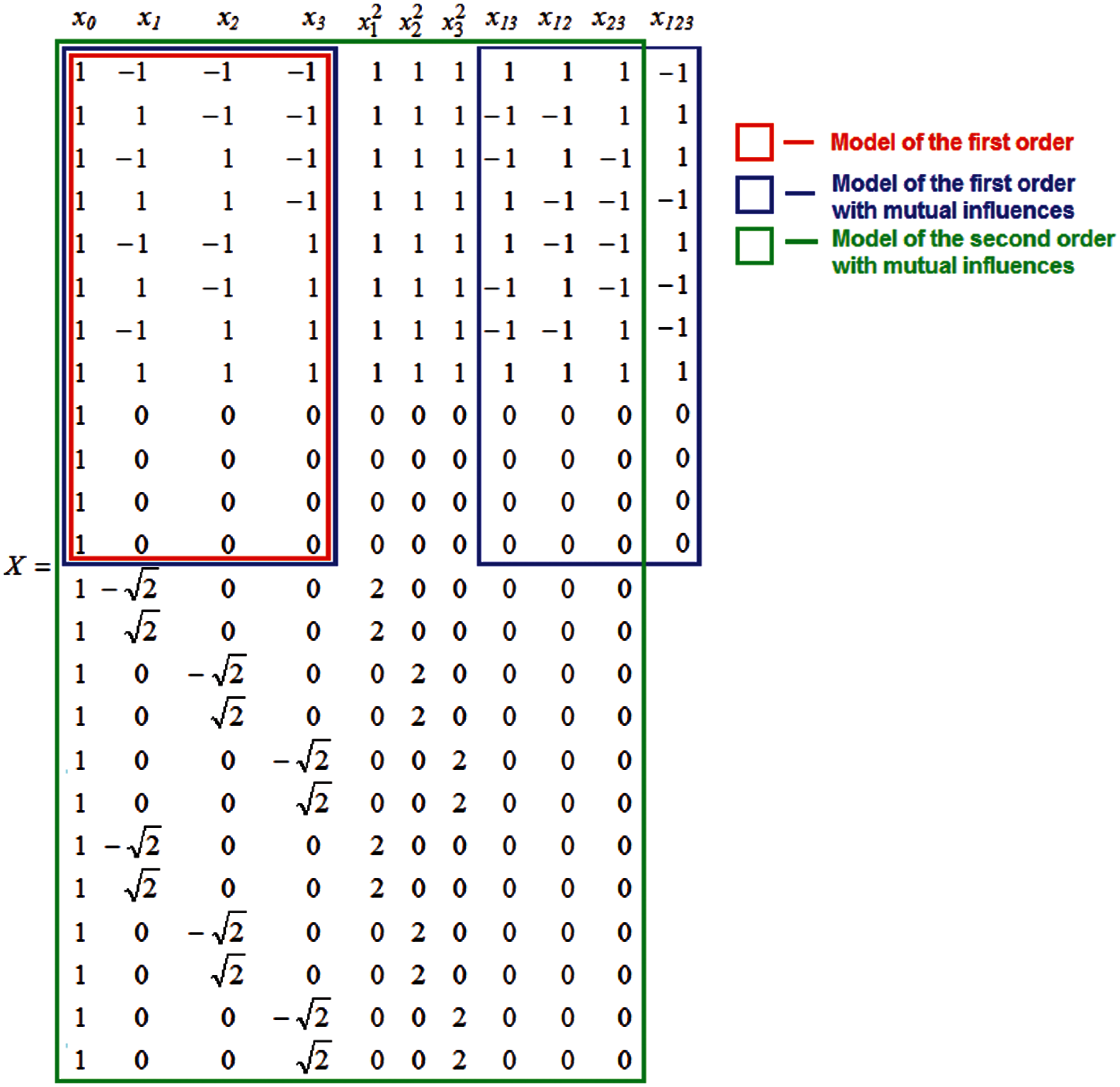
Figure 1: Matrix plan

The functional dependence of the three examined parameters on the response variable, with different types of models, is represented by Eqs. (40)–(42).

R=CF1p1F2p2F3p3,(40)

R=CF1p1F2p2F3p3exp⁡(p12ln⁡F1ln⁡F2+p13ln⁡F1ln⁡F3++p23ln⁡F2ln⁡F3+p123ln⁡F1ln⁡F2ln⁡F3),(41)

R=CF1p1F2p2F3p3exp⁡[p11(ln⁡F1)2+p22(ln⁡F2)2++p33(ln⁡F3)2+p12ln⁡F1ln⁡F2++p13ln⁡F1ln⁡F3+p23ln⁡F2ln⁡F3].(42)

where independent variables are represented by Fi and dependent variables by R.

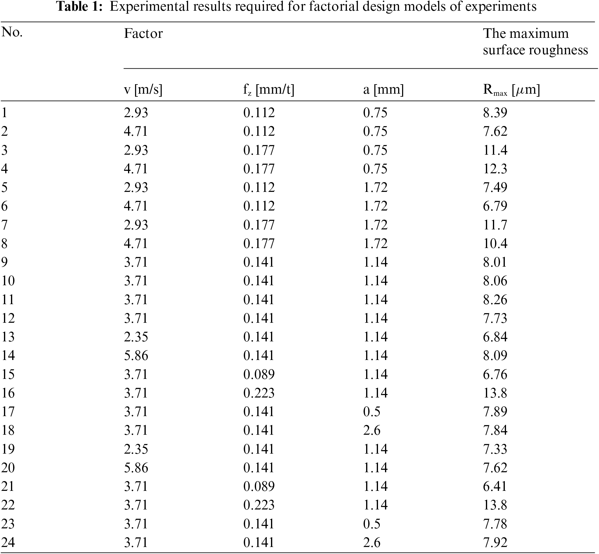
Example: Roughness of the machined surface during face milling depending on the cutting speed (v), feed per tooth (fz ) and cutting depth (a)

Tab. 1 shows the matrix plan for the maximum surface roughness for the three-factor plan of the second work previously shown in Fig. 1. The presented results were obtained experimentally by combined face milling, with a milling head with a diameter of 100 mm and inserted hard metal plates of quality class K20. Aluminum alloy 7075 with 4.4% Cu as the first alloying element was used as the processing material. Roughness measurement was performed with the help of the device “MarSurf PS1”.

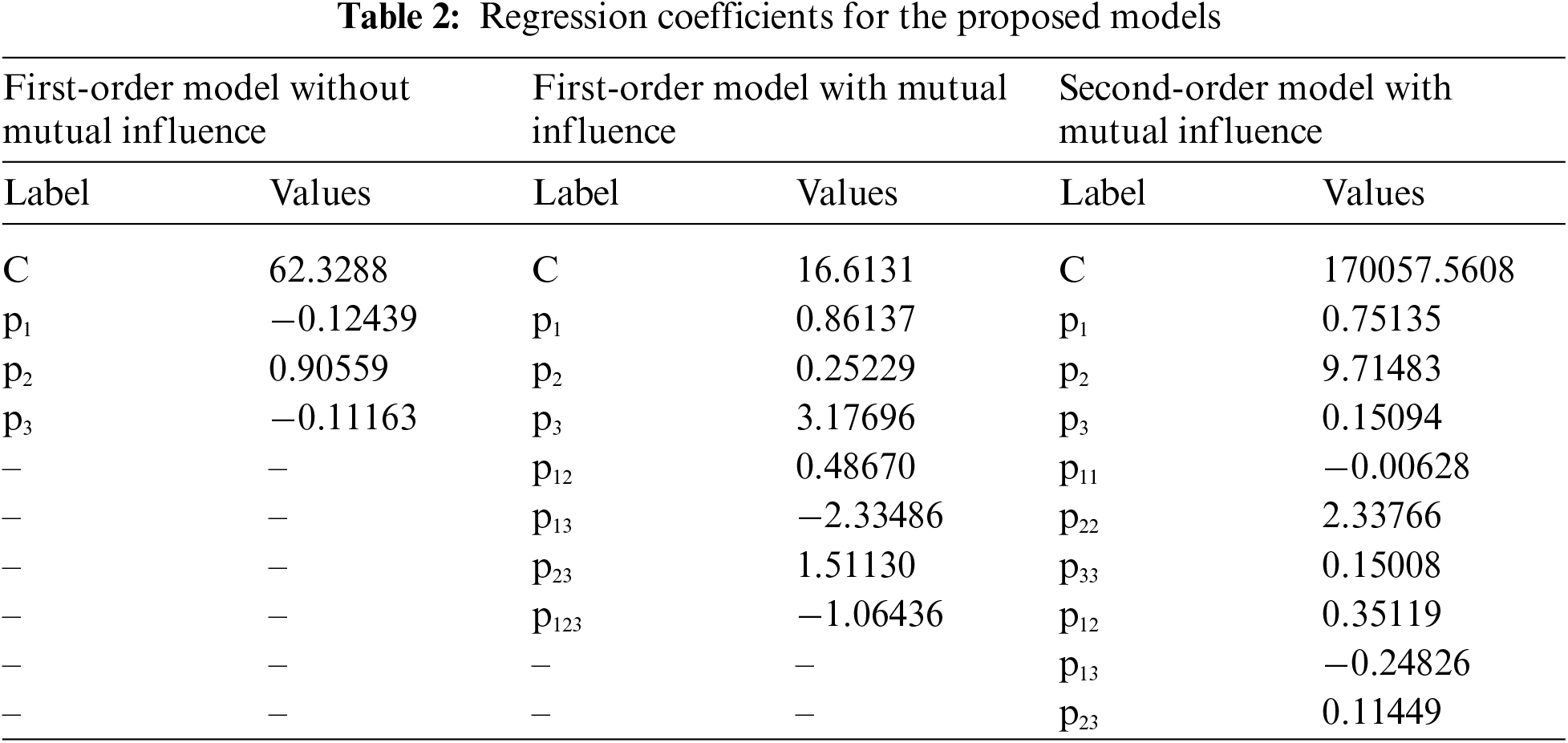
After generating the independent parameters (v, fz and a) and the dependent variable Rmax in Eqs. (40)–(42), the proposed models have the following form:

Rmax=Cvp1fzp2ap3,(43)

Rmax=Cvp1fzp2ap3exp⁡(p12ln⁡vln⁡fz+p13ln⁡vln⁡a++p23ln⁡fzln⁡a+p123ln⁡vln⁡fzln⁡a),(44)

Rmax=Cvp1fzp2ap3exp⁡[p11(ln⁡v)2+p22(ln⁡fz)2++p33(ln⁡a)2++p12ln⁡vln⁡fz++p13ln⁡vln⁡a+p23ln⁡fzln⁡a].(45)

After mathematical data processing, i.e., coding of independent variables, i.e., decoding according to the previously presented model, the following coefficients are obtained in the proposed regression equations, Tab. 2.

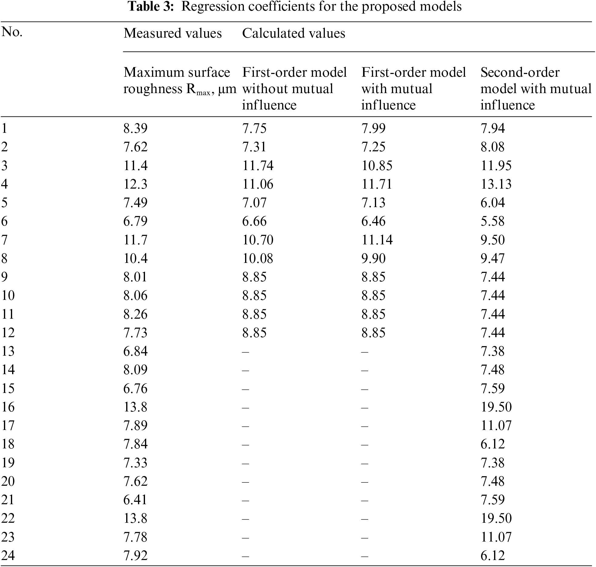
By applying the proposed models, it is possible to obtain the calculated values for the dependent variable, i.e., to select the most favorable model. In that sense, it is possible to calculate the adequacy of the appropriate model or the percentage deviation of the obtained values in relation to the experimentally read ones. The user of these models, depending on which model describes the experimental values more closely, has the open possibility of choosing the most relevant model.

Tab. 3 shows the values of the experimentally obtained data for the maximum surface roughness as well as the calculated values obtained on the basis of the three discussed models. The user has the opportunity to choose the appropriate model with aspects of the test rank as well as the accuracy levels of the model.

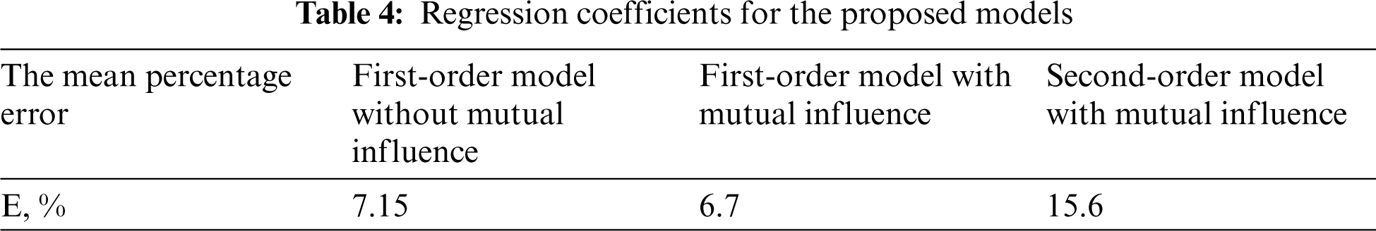
The level of accuracy, i.e., deviation can be determined on the basis of dispersion analysis where the adequacy of the proposed models would be analyzed in detail. However, a simpler way is to determine the accuracy based on the mean percentage error-E, Eq. (46), where the reliability of the models that described the corresponding output characteristics of the process can also be determined. Efforts should be made to ensure that the deviation of the data used in the training of the relevant models does not exceed 10%.

E=|Simod−Siexp|Siexp∗100%,i=1÷n,Si=Rmaxi.(46)

Tab. 4 shows the results of the percentage deviation of the error for the three presented models. Based on the results, it can be concluded that in this example it would be most appropriate to choose: First-order model with mutual influence.

If we compare the deviation of the experimental error with some similar results [23], we can conclude that we are on the right track, i.e., that the order of magnitude of the deviation is very similar. In the presented example, the worst result was obtained with the help of the Second-order model with mutual influence, however, this does not necessarily mean that it is not sufficiently applicable in the literature [19,41]. On the other hand, if some tools of artificial intelligence are applied to such mathematical models, the error of deviations will be even smaller, which can be seen from the literature [30,44].

5  Conclusions

Data modeling is an abstract view of the state of a real system, i.e., defining the data structure. A certain data model represents a simplified representation of a real system through a set of objects (entities) as well as the connection between them.

These links contain a set of information on which the relationships and relations between individual entities (variables) can be based, and thus the creation of different models.

If we look at the modeling of functions and their application, it can be concluded that the field is very wide, i.e., it can be applied as in social, natural or technical technological sciences.

The process of applying mathematical models to experimental results can be very complicated and time consuming if the appropriate stages in model formation are not performed. Great relief is obtained by the coding process, where the experimental values are reduced to prime numbers which contribute to the formation of simpler forms of equations. After selecting the most favorable mathematical model, it is necessary to perform decoding and return to the original values of the variables. If these coding and decoding procedures are skipped, the process of equation formation is very long and extensive. This paper contributes to the formation and application of models to experimental results.

Observing the presented example that deals with modeling the machinability functions of the milling process, i.e., the parameters of the machining regime and the output characteristics of the process state, the preconditions for predicting, managing and optimizing the machining parameters are created. The modeling process was performed with the help of mathematical models obtained on the basis of multifactor regression analysis. The obtained models can be analyzed in parallel and for each function the adoption of the most favorable model can be proposed from the aspect of obtaining the smallest possible deviation error from the experimental values. It is also possible to verify the accuracy of the model based on additional experiments, which were not previously used in their implementation.

Funding Statement: The authors received no specific funding for this study.

Conflicts of Interest: The authors declare that they have no conflicts of interest to report regarding the present study.

This work is licensed under a Creative Commons Attribution 4.0 International License, which permits unrestricted use, distribution, and reproduction in any medium, provided the original work is properly cited.