DOI:10.32604/cmc.2022.021839
| Computers, Materials & Continua DOI:10.32604/cmc.2022.021839 | |
| Article |
Course Evaluation Based on Deep Learning and SSA Hyperparameters Optimization
Department of Computer and Systems, Faculty of Engineering, Mansoura University, Mansoura, 35516, Egypt
*Corresponding Author: John FW Zaki. Email: jfzaki@mans.edu.eg
Received: 16 July 2021; Accepted: 01 September 2021
Abstract: Sentiment analysis attracts the attention of Egyptian Decision-makers in the education sector. It offers a viable method to assess education quality services based on the students’ feedback as well as that provides an understanding of their needs. As machine learning techniques offer automated strategies to process big data derived from social media and other digital channels, this research uses a dataset for tweets' sentiments to assess a few machine learning techniques. After dataset preprocessing to remove symbols, necessary stemming and lemmatization is performed for features extraction. This is followed by several machine learning techniques and a proposed Long Short-Term Memory (LSTM) classifier optimized by the Salp Swarm Algorithm (SSA) and measured the corresponding performance. Then, the validity and accuracy of commonly used classifiers, such as Support Vector Machine, Logistic Regression Classifier, and Naive Bayes classifier, were reviewed. Moreover, LSTM based on the SSA classification model was compared with Support Vector Machine (SVM), Logistic Regression (LR), and Naive Bayes (NB). Finally, as LSTM based SSA achieved the highest accuracy, it was applied to predict the sentiments of students’ feedback and evaluate their association with the course outcome evaluations for education quality purposes.
Keywords: Sentiment analysis; course evaluation; deep learning; Bi-LSTM; opinion mining; students feedback; natural language processing; machine learning; tweets analysis; SSA
Sentiment analysis is a natural language processing technique used to assess whether the information is negative, positive, or neutral. Sentiment analysis is frequently performed on text-based information to help organizations screen brands and assess their items and services based on the customers’ feedback and understanding customers’ needs [1]. Currently, machine learning techniques are continually being used to provide deep understandings of what people express through social media. Data analysis, which is acquired from news reports, user reviews, social media, customers’ surveys, or microblogging, can also be called opinion mining. People sentiments, in general, are gathered and used by researchers to perform assessments and guide them for the right strategic decisions [2].
The Egyptian government directs many resources towards public services to improve the quality of life on Egyptian soil. From that prospect, it is important to infer people's opinions about the different services and facilities for continuous improvement in many of its economic sectors. An automated strategy to understand such sentiments is necessary to help better planning future services through applying several machine learning methods on a standard tweets dataset and finally compare their relative accuracy measures [3]. The proposed research represents a paradigm to utilize sentiment analysis methodologies in a predefined sequence of steps to achieve accurate prediction of students’ education quality feedback to assess such important public service activity in a time that hybrid learning plays an important role in education [4].
Many researchers have used sentiment analysis in different aspects of life. Research by Hermanto et al. [5] investigated the tourism sector in Indonesia, which is influenced by the innovation that affects the freedom to access data. A tweet as an online media that reflects tourists' emotions has the chance to reveal information about the traveler locations that they will or already have visited, such as tourists’ experience, tourists’ feedback on a place of interest, and other vacation destinations. The Naive Bayes method was utilized to estimate the likelihood of every sentiment. Their research assessed people's emotions and classified them into two classes, which are positive and negative. Accordingly, it can guide travelers and tourists to suitable tourist destinations and help decision-makers improve such an important economic sector.
Another research has surveyed the sentiment analysis techniques and is composed of four fundamental phases. First, the dataset collection phase in which the Twitter API is utilized to extract the dataset with positive and negative sentiments that characterize the different tweets. Second is the preprocessing of tweets, wherein a preprocessing step is performed for removing the slang words and the incorrect spellings before extracting the features. The slang word dictionary is made utilizing the domain information. Third, the formation of a feature vector in which explicit features like hashtags and emotions were extracted. Based on the polarity they represent feelings are assigned specific weights with “1” being the weight for positive feelings while “−1” is the weight for negative feelings. Fourth is the sentiment analysis in which the features vector was classified using standard classifiers followed by an ensemble classifier with better accuracy [6].
Recently, sentiment analysis is heavily applied in the education domain, specifically students’ feedback and responses to course quality surveys. This is a complicated and daunting task due to students' dialect and expressions and the amount of data that must be processed. Therefore, sentiment analysis remains challenging despite the growing number of conducted research. Many researchers approached the domain of sentiment analysis from various perspectives. Nevertheless, the comprehensive literature reviews that analyze, sort, and classify the results of the different algorithms involved with sentiment analysis in the education domain are limited. Algorithms such as deep learning (DL), big data (BD), machine learning (ML), and natural language processing (NLP) represent the main direction for achieving better accuracy. In research developed by Kastrati et al. [7], they studied the structure of published research and presented a mapping of the available results. The paper identified 92 education-relevant studies focusing on students’ feedback regarding their learning management systems from 2015 to 2020. These relevant results were found among 612 research papers that were initially identified in the publications. The paper showed that, despite the challenges, sentiment analysis is growing particularly the deep learning techniques. The gaps in the body of literature, such as emotional expressions detection and structured datasets, were identified. The focus on such techniques will assist in the progress and advancement of the research in the field.
With the increased social media user-generated content, particularly Twitter, the growing need for tweets sentiment analysis became apparent. That is, the analysis of the emotional status and mood of the users tweeting about a certain topic. Therefore, many researchers tackled tweet sentiment analysis aiming to improve the practical performance of the approaches used. Thus, applying their algorithms for recommendation systems applications and decision support systems. While many approaches focused on enhancing the performance using the feature ensemble method, they neither considered the sentiment context of the words nor the fuzzy sentiment. Rather frequently, they focused on semantic meaning. The fuzzy sentiment approach proposed by Phan et al. based on feature ensemble considered parameters such as word sentiment polarity, lexical and linguistic elements, and type and position of the words. They implemented the approach on real data with improved sentiment analysis performance [8].
As online shopping is currently a trend, especially after COVID-19, where the sales of big giants like Amazon soared, sentiment analysis of product reviews on eCommerce websites can dramatically increase the quality of service and thus user satisfaction. Yang et al. newly proposed research used data from the Chinese eCommerce platform dangdang.com after crawling and cleaning it. The research combined convolutional neural networks (CNN) with a bidirectional gated recurrent unit (GRU). The method named model-SLCABG used deep learning and sentiment lexicon to improve currently used sentiment analysis for product reviews. The algorithm used a sentiment lexicon to improve the sentiments in the product reviews. This is followed by the CNN & GRU to extract sentiment and context features. Then, classify the weighted sentiments based on the attention mechanism, which showed an enhanced sentiment analysis performance [9].
A few research directions have utilized evolutionary optimization techniques to optimize long short-term memory (LSTM) hyperparameters and other deep learning architectures [10]. Almalaq and Zhang proposed a deep learning method for reducing building energy consumption using a predictive model. Their paper showed that the surveyed prediction methods were heavily dependent on the developer’s expertise to set the hyper-parameters. Thus, showing that for better prediction, the learning hyper-parameters of the network should be fine-tuned. Their proposed algorithm combined a genetic algorithm with LSTM. They used the number of hidden neurons and time-window lags to optimize the objective function. They tested the optimized predictive model on residential and commercial buildings from a public building dataset for very short-term prediction. Their evolutionary predictive model showed better results in comparison to the conventional prediction models [11].
Recently, in the education sector, particularly with COVID-19, many organizations were forced to opt-out of conventional education to online education. With this change happening quickly in many developing countries lacking infrastructure and technologies, many academics and students alike were resistant to this change. It became more important than ever to measure the students’ feedback and emotions. Until very recent days, many researchers worked on the identification of students’ emotions using some conventional methods. However, deep learning models, especially LSTM with attention layers, have gained more momentum to analyze students' emotions. Recent research by Sangeetha and Prabha, parallelly processed sequences of phrases across attention layers utilizing Glove and Cove embeddings. The data out of the multi-layers were fused and fed to the LSTM layer. They experimented various dropout rates to improve the accuracy. The research concludes that LSTM with fused multilayer outperforms common methods [12].
While research by Kastrati et al. emphasized the fact that to gain invaluable insights about the learning process, the organizations must analyze the feedback collected from students. The process could be very simple to be handled manually by a human for courses that have few students enrolled. Nevertheless, analyzing such emotions becomes impractical for courses with large number of students enrolled. For instance, online courses which are delivered through massive open online course platforms (MOOCs) [13].
Therefore, this paper proposes a framework to analyze the feedback from students. The methodology targets aspect-level sentiment analysis. It uses opinion polarity regarding a particular aspect in the unlabeled students’ feedback and propagates the signals to classify the aspect category. Thus, dramatically reducing the need for labeling data which is the deep learning major bottleneck. That could be achieved by utilizing a pre-trained predictive system based on a labeled dataset similar to the type of writing students might use in their feedback comments with high classification accuracy.
The layout of this research contains the following sections. Section three introduces the materials and methods employed in this research. Section four presents the prediction results, discusses the classification accuracy, and shows the application of the classifier with the highest accuracy to the students’ feedback analysis. The paper concludes in Section five.
The first stage conducted in this research is the dataset selection of tweets’ sentiments with three classes. The second stage is the preprocessing of the Twitter dataset to remove symbols, perform Stemming and Lemmatization followed by normalizing the extracted features from the tweets dataset. Several classifiers can be applied to predict the tweet’s corresponding sentiment, either positive or negative. The classification step can apply several machine learning models such as Naive Bayes, Support Vector Machines, and Logistic Regression. This research will use those techniques to represent commonly used classifiers to evaluate the proposed automated classification method as shown in the process in Fig. 1.
The Twitter dataset contains 163k tweets along with its sentimental labeling. All the comments in the dataset are cleaned and assigned with a sentiment label using Textblob. The tweets dataset can be used to build a sentimental analysis machine learning model. The dataset is collected from the tweets posted on Twitter. To collect the dataset, the Twitter API is utilized to extract the tweets. The dataset investigated different parts of sentiment analysis classification. Other technologies such as Amazon EC2, Google Visualization, Google Charts, Google Sites, Google spreadsheets, Google Closure, and Google Analytics were utilized. In this approach, any tweet with positive feelings, like “:)”, were considered positive, and tweets with negative feelings, like “:(“, were considered negative. In each record created through a tweet, information such as tweet id, text, client name, and so on can be extracted [14]. The data file format has 2 fields: ‘0’ is the text of the tweet, and ‘±1’ is the polarity of the tweet where (0 = neutral, −1 = negative, and +1 = positive).
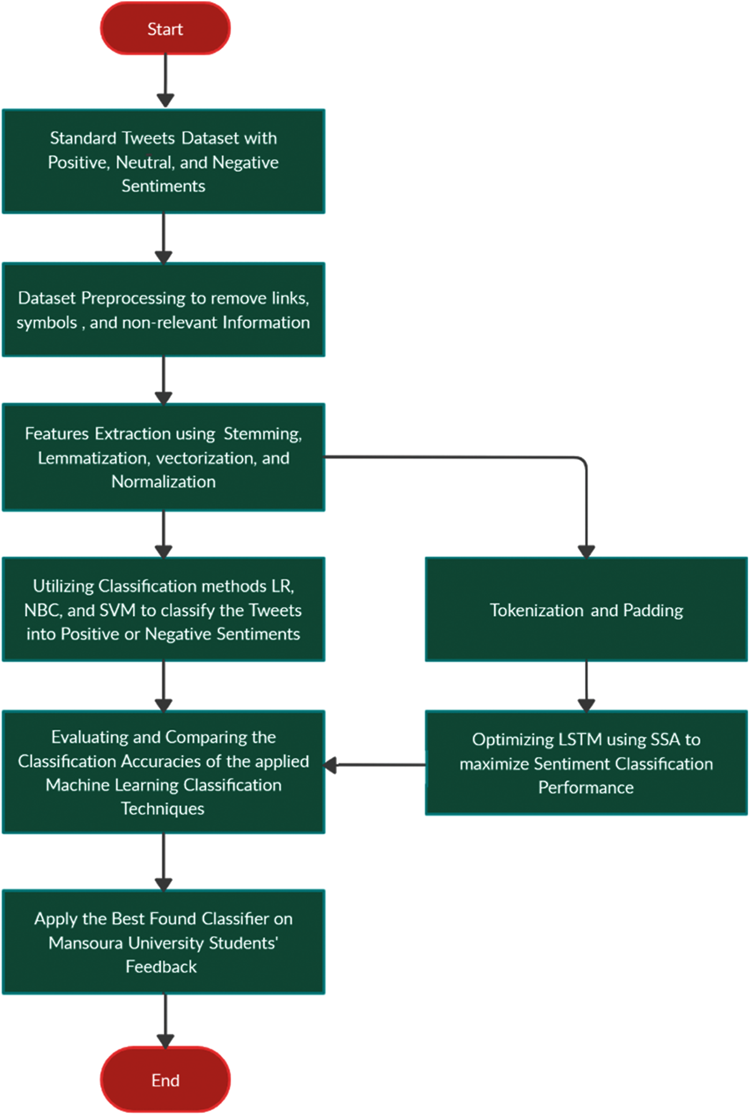
Figure 1: Flow chart for sentiment analysis
The dataset consists of 162969 tweets with negative, neutral, and positive sentiment. The tweets that correspond to positive sentiments have a size of 72249 tweets the negative sentiment have a size of 35509 tweets while the neutral sentiment has a size of 55211 tweets. Therefore, the standard dataset is balanced. The following Fig. 2 is the pie chart of negative, neutral, and positive tweets samples.
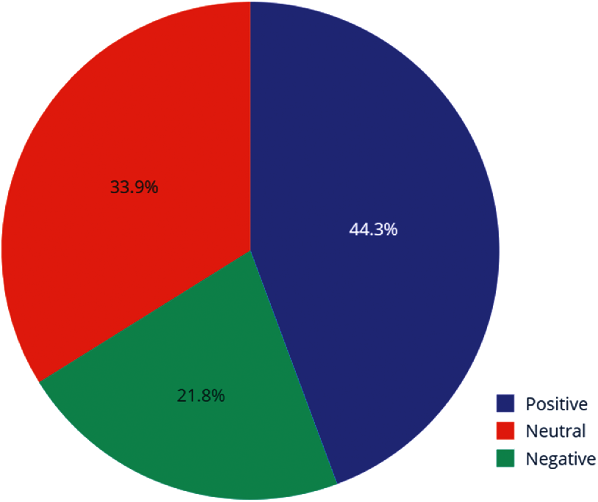
Figure 2: Pie Chart of the different sentiments of the tweets
The text needs to be cleaned, dividing it into words and taking care of case and punctuation. Indeed, an entire set of text preprocessing strategies may have to be utilized, and the selection of the right method relies upon the natural language processing task. The initial phase in cleaning up text is to have a solid idea regarding what we are attempting to accomplish, and in that setting, review text to perceive what precisely may help. Filtering out regular expressions, markups, new lines, punctuations, hyphenated descriptions, dashes, names, and markers are considered the first step to process the tweets’ text. The text cleaning frequently implies a list of words that can be utilized in the machine learning models. This implies changing over the text into a list of words.
The approach for preparing the classification algorithms input is word embedding. It includes Word2vec utilizing models such as skip-gram and continuous bag-of-words (CBOW). Skip-gram tries to predict the words surrounding a given target word, usually in the center of the context. Continuous bag-of-words does exactly the reverse of that. It predicts a word that is likely to occur in a particular context.
Stop words are the words that are filtered out which do not contribute to the deeper meaning of the sentence. Usually, they are the most common words in the language such as “the “, “a“, and “is“. They do not add sentiment information to the tweets. For sentiment analysis, it may make sense to remove the stop words. That step can be achieved by comparing each word to the stop words and filter them out [15].
3.3.3 Stemming and Lemmatization
Stemming is the way toward reducing each word to its root or base. For instance, “fishing”, “fished”, “fisher” all can be reduced to the stem “fish”. Sentiment analysis may benefit from stemming by decreasing the vocabulary and concentrating on the sentiment of a tweet instead of deeper meaning. There are many stemming techniques, although the most common and long-standing technique is the Porter Stemming algorithm. While lemmatization refers to doing things appropriately with the utilization of a vocabulary and morphological analysis of words. This regularly intends only to eliminate inflectional endings and return dictionary form of a word known as the “lemma”. Both stemming and lemmatization may likewise vary in that stemming most normally falls into derivationally related words, while lemmatization collapses the distinctive inflectional forms of a lemma [16]. The word clouds for the negative, neutral, and positive sentiments are shown in Fig. 3.

Figure 3: Word cloud plot for the three sentiments in the tweets dataset, (a) Positive sentiment words, (b) Negative sentiment words, and (c) Neutral sentiment words
3.3.4 Tokenizing, Sequencing, and Padding
The process of converting text to vectors through tokens is known as tokenization. It is also easier to filter out unnecessary tokens. Padding is used in sentiment analysis to make the input data sample of consistent size. Frequently, the zero-padding operation is used to fill a zero in the missing position. Thus, padding sentences to a fixed length for text classification using Bi-LSTM as illustrated by Ali et al. [17]. Herein, text tokenization into sequences of integers, then padded to the same length and used as input to the classifier.
This paper evaluates the model using accuracy, precision, recall, and F1 score [18]. They are consistent with metrics used in other research papers. The calculation parameters are defined as follows:
• True Positive (TP): the number of positive tweets predicted as positive.
• False Positive (FP): the number of negative tweets predicted as positive.
• True Negative (TN): the number of negative tweets predicted as negative.
• False Negative (FN): the number of positive tweets predicted as negative.
Accuracy: correctly predicted tweets divided by the total tweets.
Precision: correctly predicted positive tweets divided by the total predicted positive tweets.
Recall: correctly predicted positive tweets divided by all tweets in an actual class.
F1: the weighted average of precision and recall.
Salp Swarm Algorithm (SSA) is a class of swarm-based algorithms that belongs to metaheuristic techniques. Salp swarm species have similar features and behaviors. For instance, searching for food, locomotor performance, and communication methods. Salp belongs to the family of salpidae. It is very similar to jellyfish; barrel-shaped and moves by contracting and pumping water through their gelatinous bodies to move. They feed through internal feeding filters. Fig. 4 shows a group of salps arranged in a salp chain. This arrangement is believed to help salps achieve better locomotion and foraging [19].
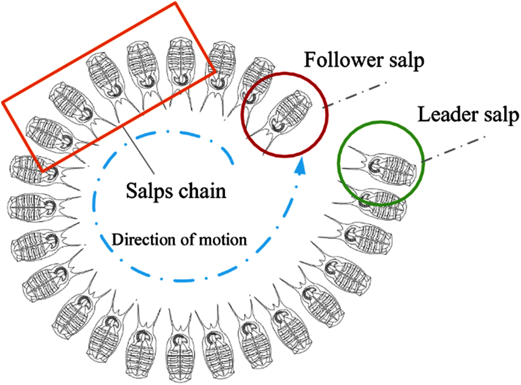
Figure 4: Salp chain composed of a leader salp and followers
SSA, proposed by Mirjalili et al., is an optimization method based on population. The SSA behavior is deemed convincible by comparing it with the salp chain foraging for optimal food sources. That is, the ability to improve the initial random solution and converging towards the optimum (assuming the target of this swarm is an optimum food source in the search space called F). In the SSA chain, the salps are either leaders or followers based on their individual position in the chain. The chain starts with a leader who guides the movements of the followers [20]. When implementing SSA, the leader’s position is updated using the following proposed Eq. (5):
where,
S2, S3 are uniformly generated random numbers in the interval [0,1].
From Eq. (5), the salp chain leader’s position is updated with respect to the food source position. The random number S1 is used to balance exploration and exploitation, with Lc being the current number of iteration and LM being the maximum number of iterations, as shown in Eq. (6):
where the S1 parameter is controlled through Lc such that the initial steps of the optimization problem are diversified while the final steps are intensified. While the previous equations show the position of the leader, the followers’ position is updated [21] as shown in Eq. (7):
where
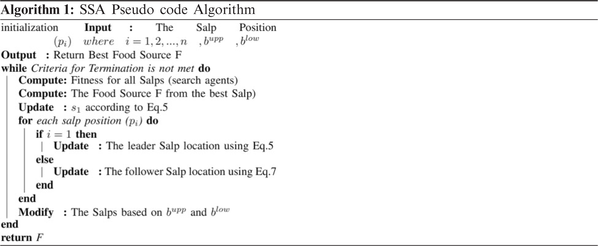
The following pseudo-code algorithm explains the main steps of the SSA and how some of the proposed hyperparameters associated with the Bi-LSTM are optimized.
Classification is an area of AI that takes raw data and classifies it to a specific class dependent on the necessary features. A utilization of computational linguistics is recognized as Natural Language Processing (NLP). With the assistance of NLP, the content can be analyzed. A sentiment is known as the inference of emotions and thoughts of any individual’s opinion. The opinion is classified among positive, neutral, and negative by utilizing a supervised machine learning algorithm. In this research work, Logistic Regression (LR), Support Vector Machine (SVM), and Naive Bayes (NB) classification models are utilized.
Logistic regression is a measurement model used to show the probability of a particular class or existing event. This can be generalized to cover multiclassification. Logistic regression is the right regression model for binary classification. Like all regression analysis strategies, logistic regression gives insight for datasets, and clarifies the relations between one dependent binary variable and one or more independent variables that are interval, nominal, ordinal, or ratio-level [22]. Sometimes logistic regressions are hard to interpret; the intelligent statistical tool can undoubtedly permit the proper analysis and interpretation of the result [23].
A Support Vector Machine (SVM) is a supervised algorithm that belongs to machine learning techniques that can be utilized for both classification and regression applications. SVMs are generally utilized for classification purposes and are considered one of the most used classification techniques.
SVMs rely upon discovering a hyperplane that best partitions a dataset into two classes. Support vectors are those data nearest to the hyperplane. The dataset points that whenever a point is eliminated, would change the position of the hyperplane. Moreover, they can be seen as the essential parts of the dataset [24].
Bayesian theory is fundamentally a structure for settling on a decision under uncertainty which is a probabilistic way to deal with prediction. Bayes hypothesized that the likelihood of future events could be determined by deciding their prior recurrence.
The advantage of the Bayesian theory is its simplicity. The forecasts depend totally on the collected data, and the more the previous data, the better the classifier performs. Another benefit is that Bayesian models are self-adjusting. That is, when data changes, so does the outcome. One exceptionally reasonable Bayesian learning technique is the Naive Bayes Classifier. It depends on the Bayesian theory and is especially suitable when the dimensionality of the dataset is high [25].
Normally, the further the hyperplane dataset points are located, the more certain we are that they have been successfully characterized. Therefore, we need the dataset points to be as far off from the hyperplane as possible while being on the correct side. In this way, when new testing data is added, whatever side of the hyperplane it is situated will choose the class that we assign to it [5].
Recurrent Neural Network (RNN) is an extension of the multilayer perceptron with feedback [26]. It processes a variable-length sequence of inputs utilizing its internal memory to amend the neurons’ state. The RNN training is done by backpropagation. Nevertheless, it fails with long-term training of vanishing gradient descent. LSTM is a type of RNN that avoids the vanishing gradient problem as it is designed with longer-term memory (internal self-loops) to prevent backpropagation from vanishing through storing information for longer [21]. LSTMs can maintain a constant error that allows them to learn through both time and layers recursively. LSTM computational graph elements are shown in Fig. 5. Namely, the three gates: input, forget, and output gates. These gates are used to change the cell memory states through reading, writing, and erasing.
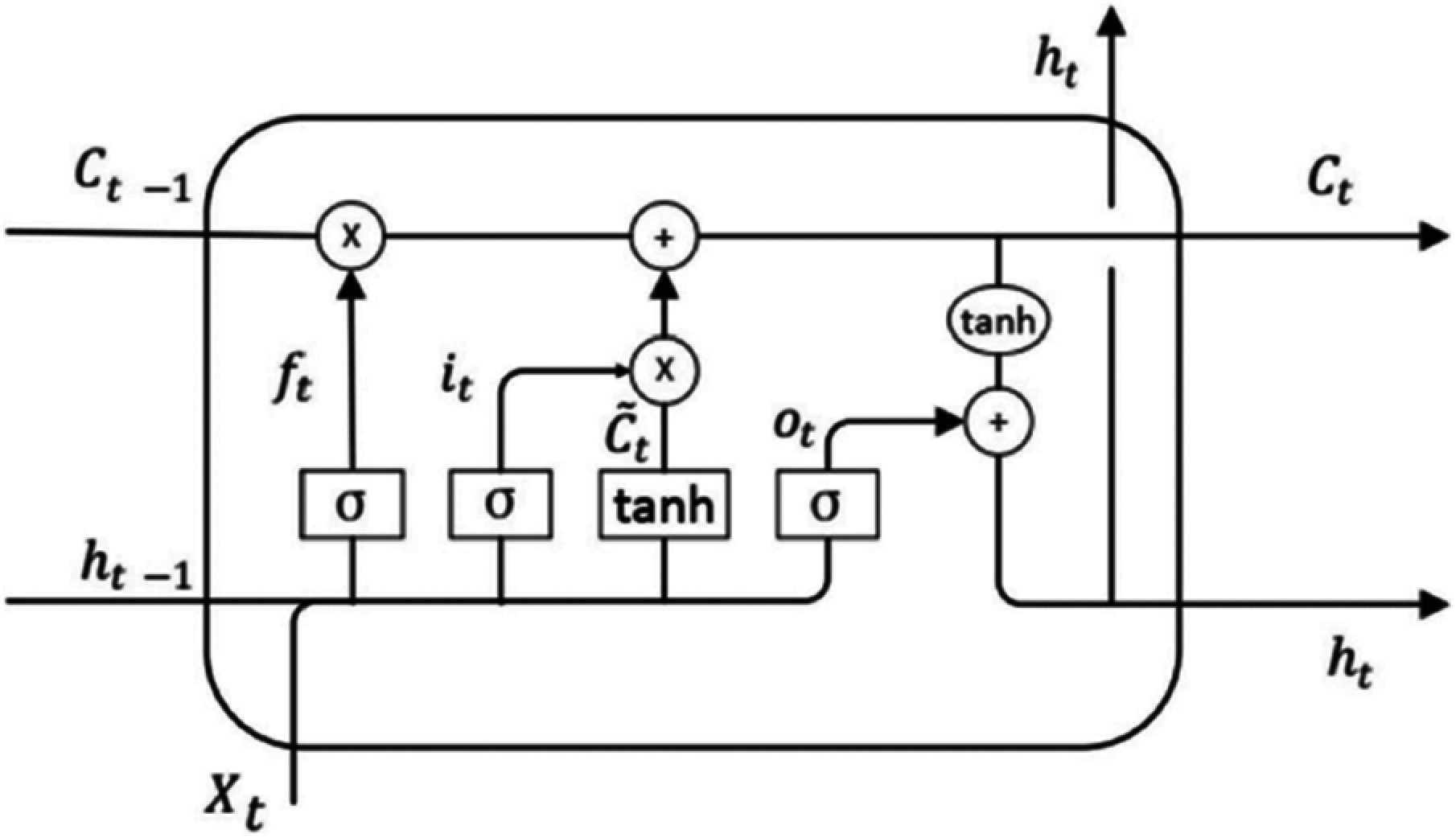
Figure 5: The LSTM architecture
where,
Thus, due to the system’s memory, each step output depends on previous inputs and calculations. Bidirectional LSTM improves the performance of sequence classification. It runs the input in two ways, from past to future and vice versa. This guarantees that information from the past and the future is preserved at any particular moment, which adds additional context to the network and results in faster and better learning of the problem [27].
The root mean squared error (RMSE) is used to evaluate the performance of the model:
There are many different search strategies to find the hyperparameters of an LSTM, such as exhaustive search, random search, and Bayesian optimization. Each one of them can affect the model performance significantly. For instance, the grid search exhaustive method attempts all possible combinations of the hyperparameters discrete subset. While this performs well with few hyperparameters, its complexity grows exponentially with the increasing number of parameters. Thus, a random search that randomly selects a subset of parameters from the set of hyperparameters is known to find better solutions in less time. On the other hand, Bayesian optimization uses previous iterations to improve the sampling of the hyperparameters for the next stage. Likewise, metaheuristic methods result in global or near-optimal solutions for hard bounded optimization problems [28]. Thus, considering the hyperparameters as shown in Tab. 1.

3.6.6 Mansoura University Use Case
Education policymakers have very few tools to help them formulate various complex policies for the socio-technical system. Thus, few researchers have modeled the different factors that affect the quality using advanced techniques such as system dynamics [29]. However, many of those factors need some form of estimation to be incorporated in the education quality models. One of those factors is the students’ feedback for basic courses, and the learning outputs can achieve aggregated sentiment analysis to assess the hybrid learning strategies set by Mansoura University committee.
Objective-type questions are utilized to gather feedback as proposed by Lin et al., through online surveys, and text descriptions [30]. Students can write textual feedback representing all the views about their learning process, as other methods limit the students’ opinions [31]. In this work, Mansoura University students’ feedback is collected through a short textual description. The proposed classifier contains positive, negative, and neutral feedback.
4.1 Predictive Models Assessment
In this section, the three commonly used sentiment analysis techniques: Logistic Regression, Support Vector Classifier, and Naïve Bayes Classifier used for the comparative study with the proposed paradigm. The proposed classifier performance comparison with other sentiment analysis techniques has been applied on the same labeled dataset.
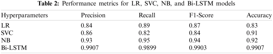
Both the training performance and architecture of the Bidirectional LSTM model are shown in Figs. 6 and 7 respectively. The normalized features dataset with the sentiment labels were used in the classification stage to detect the appropriate sentiments as measures by the testing data. The different machine learning models have achieved different classification performances, as shown in Tab. 2.
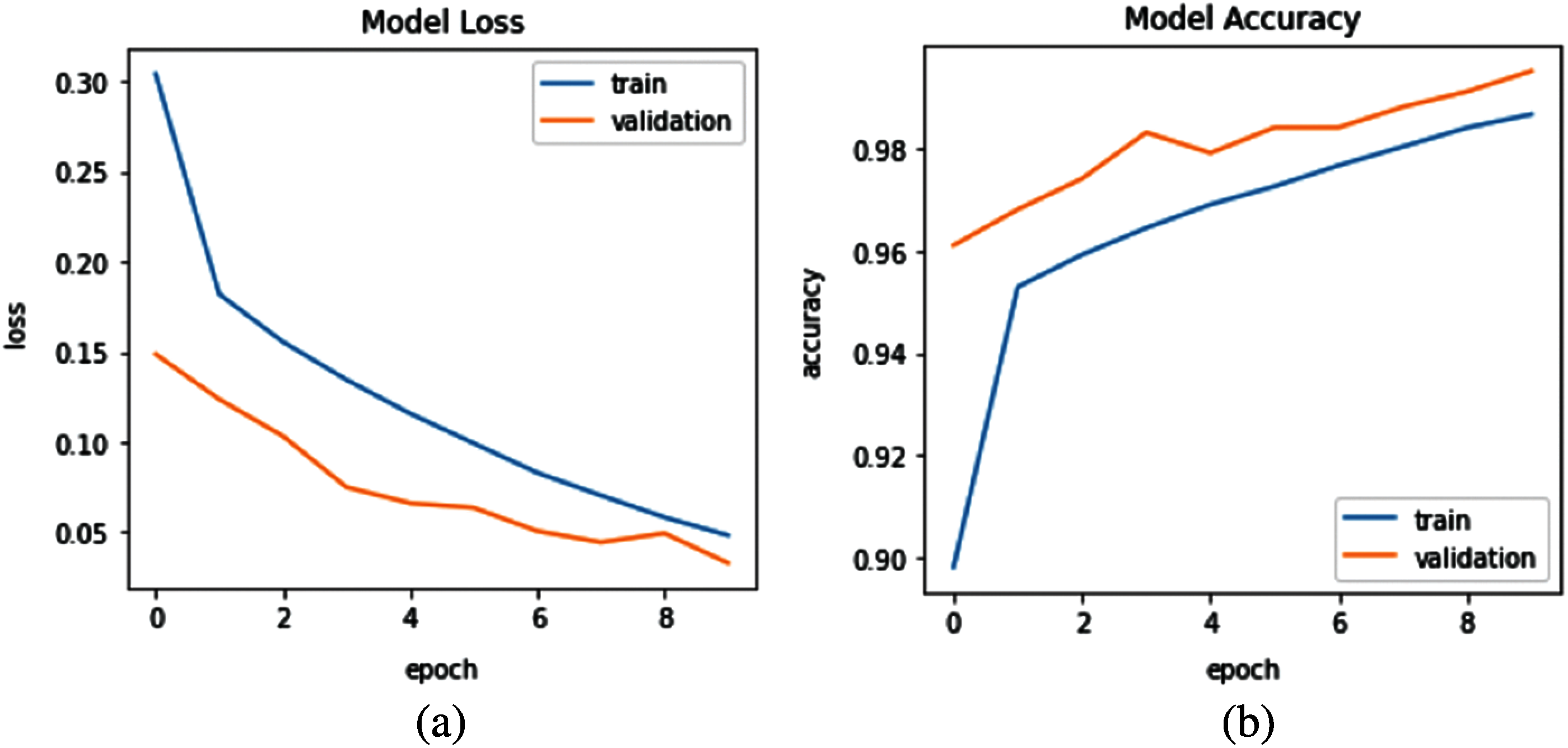
Figure 6: Model training (a) Loss, and (b) Accuracy
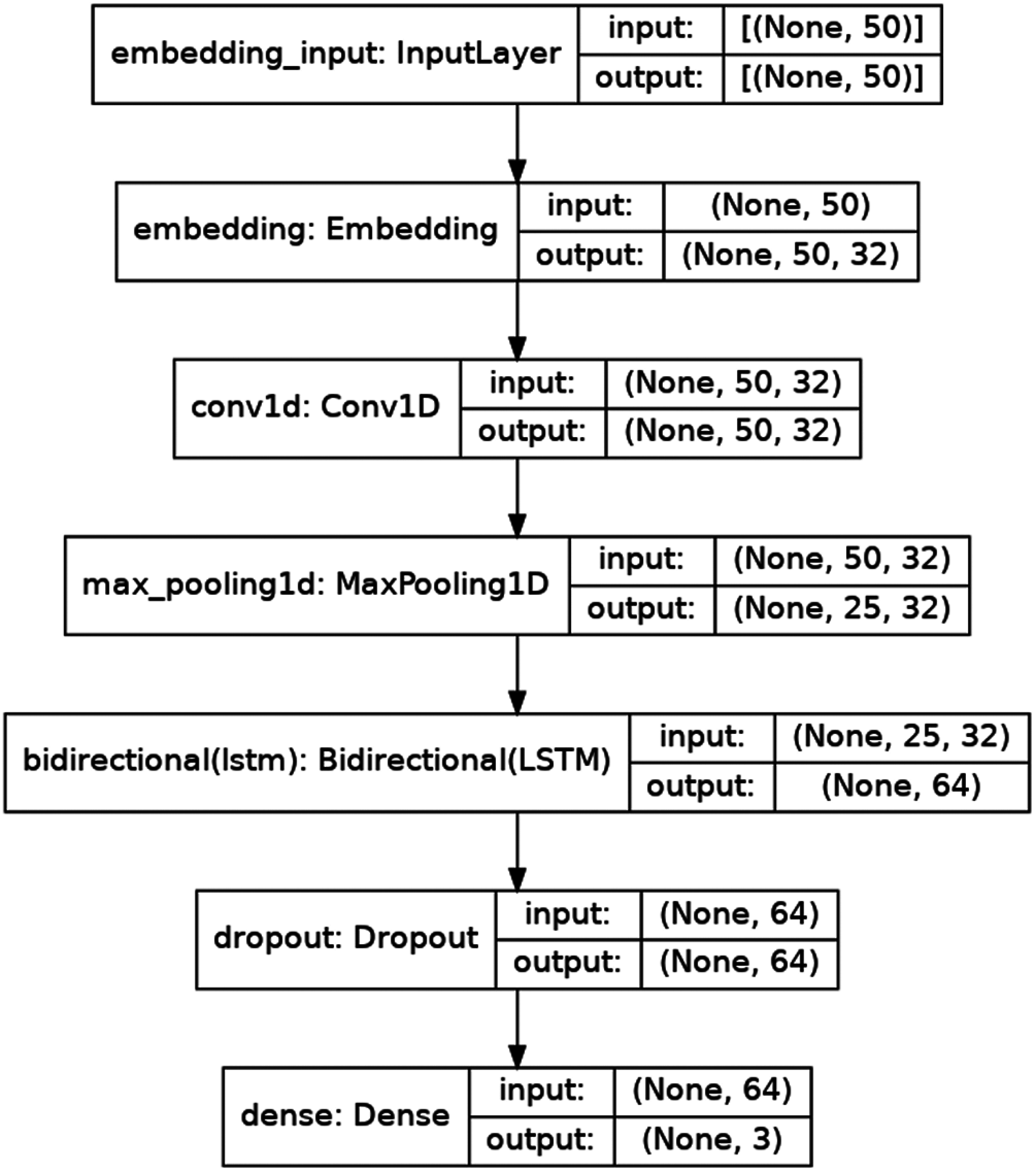
Figure 7: Bidirectional LSTM model
The logistic regression was applied to classify the sentiments of the tweets using 500 iterations, and the hyperparameters were found using the gradient descent optimization method that resulted in an accuracy of 83%. The second classifier applied a support vector classifier with hyperparameters tuned using the grid search optimization method. The support vector classifier used a linear kernel and managed to achieve an accuracy of 91%. The last applied classifier is the Naive Bayes classifier that was optimized using the grid search optimization method and resulted in 92% accuracy. The Naïve Bayes classifier technique was superior to achieving a better classification accuracy than the other commonly used techniques.
4.2 Configuration of SSA Optimization
In each iteration of the LSTM hyperparameters optimization stage, the fitness is calculated and compared with the initial fitness which is specified by LSTM performance accuracy. So that, the best fitness is obtained and stored. The outcome of the completed optimization process is a new optimized population. The number of LSTM parameters to be optimized in the SSA implementation is shown in Tab. 3. Based on time constraints and the difficulty of the problem, the population is set to 20. The SSA optimization process requires several iterations, which are specified as in Tab. 3. The LSTM optimization goal is to minimize the difference between the predicted and actual values.

The proposed classifier using Bi-LSTM has achieved a classification accuracy of 99%, which outperformed all other techniques, while its confusion matrix is shown in Fig. 8. Therefore, Bi-LSTM will be utilized in the students’ feedback sentiment analysis stage.
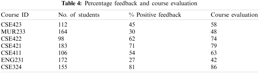
In this section, the students’ feedback sentiment analysis is assessed, and its correlation with the courses’ overall evaluation is investigated as shown in Tab. 4. The independent variable for each course is the percentage of positive feedback relative to all students’ feedback, while the dependent variable is the overall course evaluation that was statistically calculated.
In statistics, one usually measures Pearson correlation, Kendall rank correlation, Spearman correlation, and the Point-Biserial correlation. In this work, the correlation is used to measure the association between the percentage of positive feedback and course evaluation. The correlation coefficient value ranges from −1 to +1, where ±1 represents the perfect association between the variables. While the relationship weakens as the correlation coefficient approaches zero. The positive and negative signs represent the direction of the positive relationship and negative relationship, respectively.
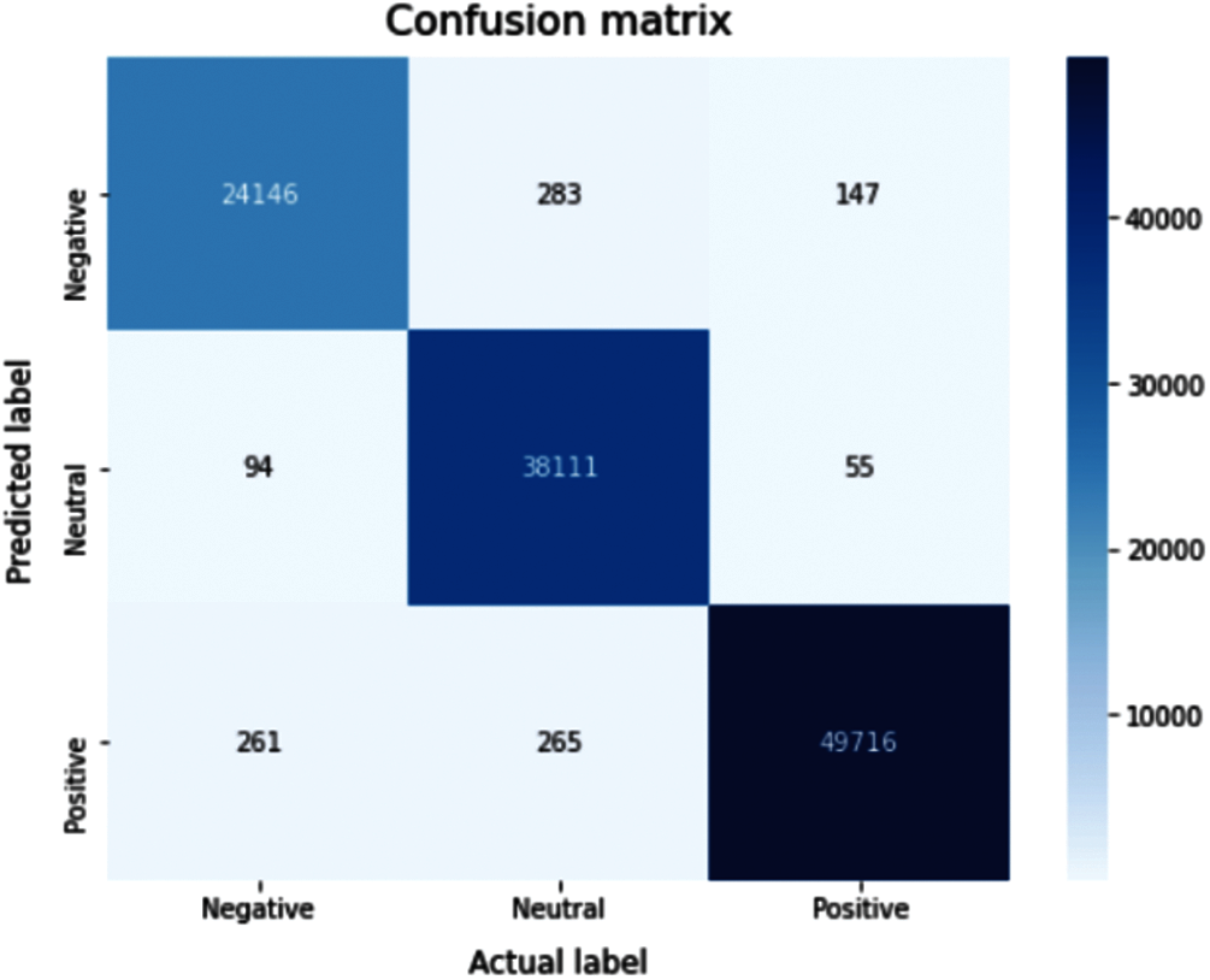
Figure 8: Confusion matrix for the proposed sentiment analysis classifier (Bi-LSTM)
In statistics, Pearson correlation is widely used to measure the relationship between linearly related variables. It is a normalized measurement of the covariance. Pearson correlation is calculated as follows:
where,
4.3.2 Kendall Rank Correlation
Kendall rank correlation measures the strength of dependency between two variables [32]. If two samples are considered where each sample size is n, then the total number of pairings is ‘n(n − 1)/2’. Kendall correlation is calculated as follows:
4.3.3 Spearman Rank Correlation
Spearman rank is used to measure the degree of association between two variables. The Spearman rank is the right correlation when the variables are measured on a scale that is at least ordinal [33]. Spearman rank correlation is calculated as follows:
n: number of observations.
4.3.4 Point-Biserial Correlation
The point-biserial correlation is conducted with the Pearson correlation formula, except that one of the variables is dichotomous [34] and used to reduce the steps in the calculations or rxy [35]. Assume that Y is the dichotomous variable with values 0 and 1. If the dataset is divided into two groups, a group with value 1 on Y and the second with value 0 on Y. Then the point-biserial correlation equation is as follows:
where Sn is the standard deviation used when data are available for every member of the population:
M1 and M0 are the mean values on the continuous variable ‘X’ for all group 1 and 2 data points, respectively.
Further, n1 and n0 represent the number of data points in group 1 and group 2, respectively, where ‘n’ is the total sample size.
The correlation coefficient is used to measure the relationship between two datasets. The p-value represents the probability of uncorrelated datasets correlating at least as high as the correlation calculated from these datasets.
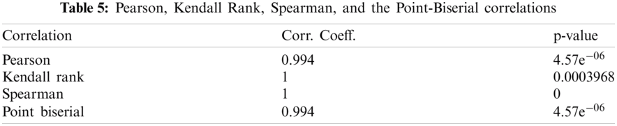
Tab. 5 shows the correlation between course feedback positive sentiment and the course evaluation based on Pearson, Kendall rank, Spearman, and the Point-Biserial correlations. Moreover, Wilcoxon Signed Rank test was calculated as a standard statistical test for correlation assessment. The p-value was found to be 0.018, which accepts the null hypothesis (H0: Means are equal).
Since online education is trending for the past few years and its use surged due to COVID-19, students’ feedback became ever so important, and educational organizations focused on improving their services through students’ opinions.
The conducted research applied an automated methodology to extract the suitable features from the different tweets to be further classified using several machine learning techniques. The features were normalized to achieve better performance. Four classifiers were applied for a comparable study, resulting in a better classification performance from a Bi-LSTM based SSA classifier. The best performing classifier namely, Bi-LSTM based SSA was applied to students’ feedback to assess different courses taught in Mansoura University using the hybrid learning scheme for sentiment analysis in the time of COVID-19 pandemic. The correlation between the percentage of the positive sentiment of each course and its course evaluation was statistically evaluated and found to be highly correlated. That in turn can be used to tweak the different strategies needed to achieve the best hybrid learning services to be adopted in the Egyptian Education System.
Funding Statement: The authors received no specific funding for this study.
Conflicts of Interest: The authors declare that they have no conflicts of interest to report regarding the present study.
1. A. E. O. Carosia, G. P. Coelho and A. E. A. Silva, “Analyzing the Brazilian financial market through Portuguese sentiment analysis in social media,” Applied Artificial Intelligence, vol. 34, no. 1, pp. 1–19, 2020. [Google Scholar]
2. M. K. S., “Social media sentiment analysis for opinion mining,” Int. Journal of Psychosocial Rehabilitation, vol. 24, no. 5, pp. 3672–3679, 2020. [Google Scholar]
3. N. Chockalingam, “Simple and effective feature based sentiment analysis on product reviews using domain-specific sentiment scores,” Polibits, vol. 57, pp. 39–43, 2018. [Google Scholar]
4. D. Wang and H. Han, “Applying learning analytics dashboards based on process-oriented feedback to improve students’ learning effectiveness,” Journal of Computer Assisted Learning, vol. 37, no. 2, pp. 487–499, 2021. [Google Scholar]
5. D. T. Hermanto, M. Ziaurrahman, M. A. Bianto and A. Setyanto, “Twitter social media sentiment analysis in tourist destinations using algorithms Naive Bayes classifier,” Journal of Physics: Conf. Series, vol. 1140, pp. 012037, 2018. [Google Scholar]
6. D. Antonakaki, P. Fragopoulou and S. Ioannidis, “A survey of Twitter research: Data model, graph structure, sentiment analysis and attacks,” Expert Systems with Applications, vol. 164, no. 1, pp. 114006, 2021. [Google Scholar]
7. Z. Kastrati, F. Dalipi, A. S. Imran, K. Pireva Nuci and M. A. Wani, “Sentiment analysis of students’ feedback with NLP and deep learning: A systematic mapping study,” Applied Sciences, vol. 11, no. 9, pp. 3986, 2021. [Google Scholar]
8. H. T. Phan, V. C. Tran, N. T. Nguyen and D. Hwang, “Improving the performance of sentiment analysis of tweets containing fuzzy sentiment using the feature ensemble model,” IEEE Access, vol. 8, pp. 14630–14641, 2020. [Google Scholar]
9. L. Yang, Y. Li, J. Wang and R. S. Sherratt, “Sentiment analysis for E-Commerce product reviews in Chinese based on sentiment lexicon and deep learning,” IEEE Access, vol. 8, pp. 23522–23530, 2020. [Google Scholar]
10. E. M. Hassib, A. I. El-Desouky, L. M. Labib and E. S. M. T. El-Kenawy, “WOA + BRNN: An imbalanced big data classification framework using whale optimization and deep neural network,” Soft Computing, vol. 24, no. 8, pp. 5573–5592, 2020. [Google Scholar]
11. A. Almalaq and J. J. Zhang, “Evolutionary deep learning-based energy consumption prediction for buildings,” IEEE Access, vol. 7, pp. 1520–1531, 2019. [Google Scholar]
12. K. Sangeetha and D. Prabha, “Sentiment analysis of student feedback using multi-head attention fusion model of word and context embedding for LSTM,” Journal of Ambient Intelligence and Humanized Computing, vol. 12, no. 3, pp. 4117–4126, 2021. [Google Scholar]
13. Z. Kastrati, A. S. Imran and A. Kurti, “Weakly supervised framework for aspect-based sentiment analysis on students’ reviews of MOOCs,” IEEE Access, vol. 8, pp. 106799–106810, 2020. [Google Scholar]
14. S. Hussein, “Twitter sentiments dataset,” May 2021, type: dataset. [Online]. Available: http://dx.doi.org/10.17632/z9zw7nt5h2.1. [Google Scholar]
15. S. Sarica and J. Luo, “Stopwords in technical language processing,” PLOS ONE, vol. 16, no. 8, pp. e0254937, 2021. [Google Scholar]
16. I. Boban, A. Doko and S. Gotovac, “Sentence retrieval using stemming and lemmatization with different length of the queries,” Advances in Science, Technology and Engineering Systems Journal, vol. 5, no. 3, pp. 349–354, 2020. [Google Scholar]
17. Z. Ali, A. Razzaq, S. Ali, S. Qadri and A. Zia, “Improving sentiment analysis efficacy through feature synchronization,” Multimedia Tools and Applications, vol. 80, no. 9, pp. 13325–13338, 2021. [Google Scholar]
18. R. Yacouby and D. Axman, “Probabilistic extension of precision, recall, and F1 score for more thorough evaluation of classification models,” in Proc. of the First Workshop on Evaluation and Comparison of NLP Systems, Online: Association for Computational Linguistics, pp. 79–91, 2020. [Google Scholar]
19. A. Ibrahim, S. Mohammed, H. A. Ali and S. E. Hussein, “Breast cancer segmentation from thermal images based on chaotic Salp swarm algorithm,” IEEE Access, vol. 8, pp. 122121–122134, 2020. [Google Scholar]
20. S. Mirjalili, A. H. Gandomi, S. Z. Mirjalili, S. Saremi, H. Faris et al., “Salp swarm algorithm: A bio-inspired optimizer for engineering design problems,” Advances in Engineering Software, vol. 114, pp. 163–191, 2017. [Google Scholar]
21. A. A. Nasser, M. Z. Rashad and S. E. Hussein, “A two-layer water demand prediction system in urban areas based on micro-services and LSTM neural networks,” IEEE Access, vol. 8, pp. 147647–147661, 2020. [Google Scholar]
22. K. Shah, H. Patel, D. Sanghvi and M. Shah, “A comparative analysis of logistic regression, random forest and KNN models for the text classification,” Augmented Human Research, vol. 5, no. 1, pp. 7, 2020. [Google Scholar]
23. S. Buya, P. Tongkumchum and B. E. Owusu, “Modelling of land-use change in Thailand using binary logistic regression and multinomial logistic regression,” Arabian Journal of Geosciences, vol. 13, no. 12, pp. 149, 2020. [Google Scholar]
24. A. Ahmed and S. E. Hussein, “Leaf identification using radial basis function neural networks and SSA based support vector machine,” PLOS ONE, vol. 15, no. 8, pp. e0237645, 2020. [Google Scholar]
25. K. Korovkinas and P. Danenas, “SVM and Naïve Bayes classification ensemble method for sentiment analysis,” Baltic Journal of Modern Computing, vol. 5, no. 4, pp. 398–409, 2017. [Google Scholar]
26. M. Chalk, G. Tkacik and O. Marre, “Inferring the function performed by a recurrent neural network,” PLOS ONE, vol. 16, no. 4, pp. e0248940, 2021. [Google Scholar]
27. W. AlKhwiter and N. Al-Twairesh, “Part-of-speech tagging for Arabic tweets using CRF and Bi-LSTM,” Computer Speech & Language, vol. 65, pp. 101138, 2021. [Google Scholar]
28. S. Bouktif, A. Fiaz, A. Ouni and M. A. Serhani, “Multi-sequence LSTM-RNN deep learning and Metaheuristics for electric load forecasting,” Energies, vol. 13, no. 2, pp. 391, 2020. [Google Scholar]
29. S. E. Hussein and M. Abo El-Nasr, “Resources allocation in higher education based on System dynamics and genetic algorithms,” Int. Journal of Computer Applications, vol. 77, no. 10, pp. 40–48, 2013. [Google Scholar]
30. Q. Lin, Y. Zhu, S. Zhang, P. Shi, Q. Guo et al., “Sentiment Analysis of people during lockdown period of COVID-19 using SVM and logistic regression analysis Lexical based automated teaching evaluation via students’ short reviews,” Computer Applications in Engineering Education, vol. 27, no. 1, pp. 194–205, 2019. [Google Scholar]
31. Z. Nasim, Q. Rajput and S. Haider, “Sentiment analysis of student feedback using machine learning and lexicon-based approaches,” in 2017 Int. Conf. on Research and Innovation in Information Systems (ICRIISLangkawi, Malaysia, IEEE, pp. 1–6, 2017. [Google Scholar]
32. D. Gao, Y. Zhou, T. Wang and Y. Wang, “A method for predicting the remaining useful life of Lithium-Ion batteries based on particle filter using Kendall Rank correlation coefficient,” Energies, vol. 13, no. 16, pp. 4183, 2020. [Google Scholar]
33. L. Zhu, “Selection of multi-level deep features via Spearman Rank correlation for synthetic aperture radar target recognition using decision fusion,” IEEE Access, vol. 8, pp. 133914–133927, 2020. [Google Scholar]
34. F. Zinzendoff Okwonu, B. Laro Asaju and F. Irimisose Arunaye, “Breakdown analysis of Pearson correlation coefficient and robust rorrelation methods,” IOP Conf. Series: Materials Science and Engineering, vol. 917, pp. 012065, 2020. [Google Scholar]
35. D. G. Bonett, “Point-biserial correlation: Interval estimation, hypothesis testing, meta-analysis, and sample size determination,” British Journal of Mathematical and Statistical Psychology, vol. 73, no. S1, pp. 113–144, 2020. [Google Scholar]
 | This work is licensed under a Creative Commons Attribution 4.0 International License, which permits unrestricted use, distribution, and reproduction in any medium, provided the original work is properly cited. |