DOI:10.32604/cmc.2022.021849
| Computers, Materials & Continua DOI:10.32604/cmc.2022.021849 | |
| Article |
ILipo-PseAAC: Identification of Lipoylation Sites Using Statistical Moments and General PseAAC
1School of Science and Technology, University of Management and Technology, Lahore, Pakistan
2Department of Computer Science and Information Technology, Virtual University of Pakistan, Lahore, Pakistan
3Department of Biomedical Engineering, New Jersey Institute of Technology, Newark, NJ, USA
4Department of Computer Sciences, College of Computer and Information Sciences, Princess Nourah bint Abdulrahman University (PNU), Riyadh, Saudi Arabia
5Department of Economics, University of Lahore, Lahore, Pakistan
*Corresponding Author: Talha Imtiaz Baig. Email: talhabaig788@gmail.com
Received: 17 July 2021; Accepted: 18 August 2021
Abstract: Lysine Lipoylation is a protective and conserved Post Translational Modification (PTM) in proteomics research like prokaryotes and eukaryotes. It is connected with many biological processes and closely linked with many metabolic diseases. To develop a perfect and accurate classification model for identifying lipoylation sites at the protein level, the computational methods and several other factors play a key role in this purpose. Usually, most of the techniques and different traditional experimental models have a very high cost. They are time-consuming; so, it is required to construct a predictor model to extract lysine lipoylation sites. This study proposes a model that could predict lysine lipoylation sites with the help of a classification method known as Artificial Neural Network (ANN). The ANN algorithm deals with the noise problem and imbalance classification in lipoylation sites dataset samples. As the result shows in ten-fold cross-validation, a brilliant performance is achieved through the predictor model with an accuracy of 99.88%, and also achieved 0.9976 as the highest value of MCC. So, the predictor model is a very useful and helpful tool for lipoylation sites prediction. Some of the residues around lysine lipoylation sites play a vital part in prediction, as demonstrated during feature analysis. The wonderful results reported through the evaluation and prediction of this model can provide an informative and relative explanation for lipoylation and its molecular mechanisms.
Keywords: Lipoylation lysine; feature vector; post translational modification; amino acid; Mathew’s correlation coefficient; neural network
Lipoylation is one of the most meaningful elements in biology. It is a unique and highly protective lysine Post Translational Modification (PTM) present in eukaryotes and prokaryotes’ proteomics [1,2]. It plays a key role in the metabolism of aerobic bacteria and eukarya [2–6]. The type of modification used in this research is dependent on local amino acid sites in protein sequences. Lysine lipoylation sites are known to be the most impressive modification processions that can become visible in most enzymes that are relevant and present in most organisms, including mammals and bacteria [7–10].
On the other hand, lysine lipoylation sites play a significant role in protein communications and metabolic pathways [1]. According to earlier research, lipoylation is the leading cause of most diseases that exist in human beings. So, if the reasons discussed above are considered, the lipoylation biological function might be informative and helpful for us to discover molecular diseases [11].
Although most of the time, many molecular lipoylation sites stay anonymous and cannot be adequately recognised. Some of the basic steps have been taken, and computational methods have been developed for lipoylation identification. However, the experiments conducted for solving these kinds of issues are costly and time taking. The most challenging thing is to research it without discovering the lipoylation sites. This is the reason that this problem is one of the most critical topics in this field. Some sites include carbonylation, crotonylation, succinylation, glycosylation, hydroxylation, s-nitrosylation, sumoylation, phosphorylation, ubiquitination, methylation and prenylation. Figs. 1(A) and 1(B) explains the synthesis pathway, the acyl chain of octanoyl (ACP) is transferred by LipB to a conserved lysine residue on the E2. LipA catalyzes sulfur insertion. Octanoyl (E2) can be generated by the dependent ligation by LplA. Fig. 1(C) is a lipoate scavenging pathway that elaborates the primary role of LplA. It catalyzes the dependent ligation to proteins. Fig. 1(D) explains the unique approach that used in the mammalian scavenging pathway in which lipoate is combined with lipoyl-GMP. It is catalyzed by the lipoate-activating enzyme (LAE). The lipoyl-NMP transferase cannot use lipoate as a substrate.
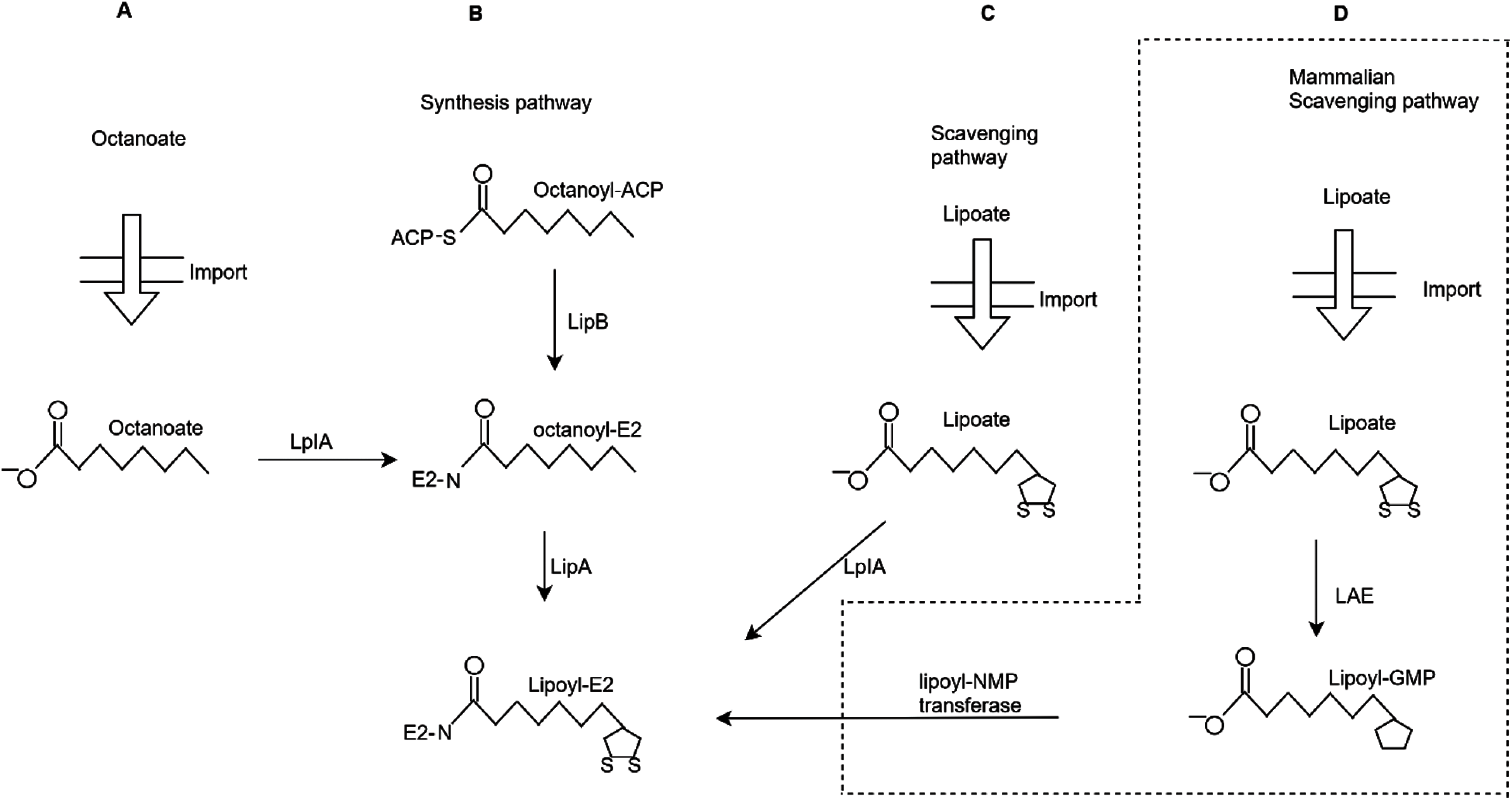
Figure 1: Different strategies of lysine lipoylation sites (A) Octanoate import (B) Synthetic pathway (C) Lipolate scavenging pathway (D) Mammalian scavenging pathway
The increasing development of lipoylation sites has highlighted many important issues. While predicting the lysine lipoylation sites, feature analysis reveals that the residue around lipoylation plays a very important role. For sample training, the algorithm used for classification is known as ANN [12]. Due to deep analysis and assessment based on many aspects, the following research shows that ANN is the most suitable technique for lipoylation site encoding compared to other extraction methods. A method has been observed to develop our predictor model known as Chou’s 5 step rule; that is, for the prediction of lysine lipoylation sites.
2 Proposed System and Methodology
The following research has discussed three different features and a method of 5 steps. The detailed method and flowchart are shown below in Fig. 2. We have designed a predictor model especially for the prediction of lipoylation sites. This model can be successfully applied in two different but many related domains like healthcare and gene expression networks. Most of the previous applications focused on the physicians and their interactions, while the latest applications cover associated genes and interactions.
The standardised dataset was collected from different sources, but the main source was UNIPROT. Our model has 500 negative dataset samples and 359 positive dataset samples. All the dataset was collected by applying some advanced level searches. Similar dataset samples were removed, and positive samples of the dataset were collected.
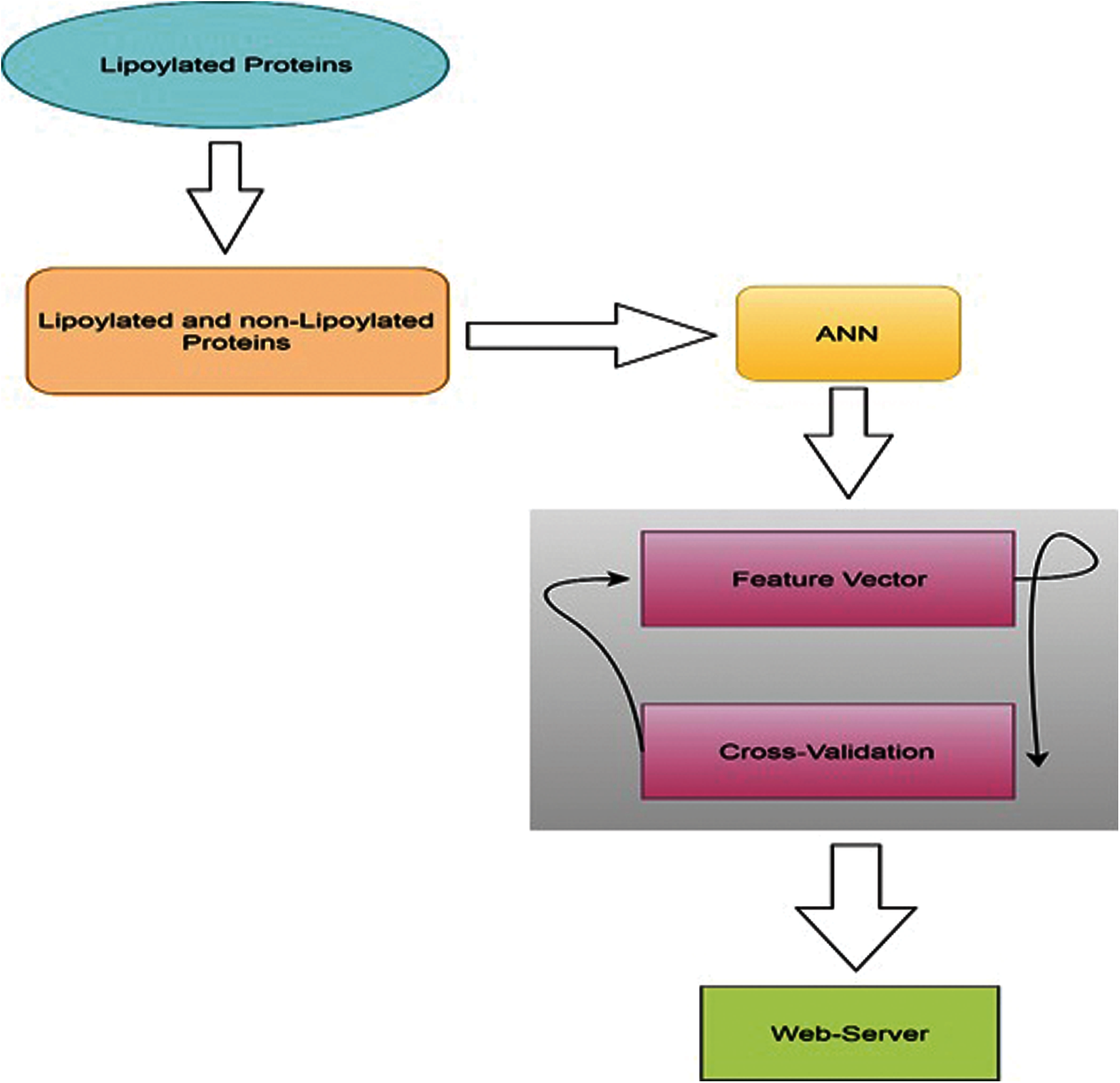
Figure 2: Methodology flowchart
By applying Chou’s formulation method [13], a peptide could be formulated as:
The length of each peptide of the collected sample was 41. Residue SPC has the following downstream location at 20, 21 residues and the upstream location at 20 residues.
where
One of the biggest problems in computational biology is formulating a discrete and vector model that includes all the information of any sequence pattern from sequence data. The important aspect of data is to derive the formation of a vector from sequence data. All the high rated algorithms of data science and deep learning such as CD algorithm as Covariance Discriminant [14,15], RF algorithm as Random Forest [16,17], Closest Neighbor algorithm or Nearest Neighbor (NN) [18,19] and SVM algorithm as Support Vector Machine [20,21] control vector input and describe them completely in detail [22]. A method is introduced to decrease the loss of sequence pattern, which is PseAAC as (Pseudo amino acid composition).
2.2.1 Calculation of SVV as Site Vicinity Vector
SVV as site vicinity vector can be the sub-sequence of the main sequence of peptides and proteins with PTM sites. Let’s assume that
The site vicinity vector is the sub-sequence of primary sequence peptide is given as
where it has minimum constant value (MCV) that is finalised by the given experiment and holds 20 value of k in this research.
2.2.2 Moments of Statistical Calculation
To define elements, dimensions and quantitative datasets for sample sequences, a moment is used called statistical moment. The moments are defined by mathematicians and statisticians using their distribution functions and polynomials theorems [23,24]. The ability of that moment is asymmetry calculation, variant and mean for the following benchmark dataset.
Using 2D transformed matrix Z’, the Hahn moment was calculated, which has the property to calculate very fast. Using Hahn moments, a calculation is done as;
In the end, probability distribution calculated the raw moments to save information that is useful for our standardised sample data set as
All 3rd degree moments are q + r and N0, N1, N2, N3, N10, N11, N12, N20, N21 and N30. These are all raw moment’s degree.
2.2.3 Frequency Vector Distribution
Every calculated amino acid frequency is saved in vector form, so it is called a frequency vector. The computation of the frequency vector is calculated as below in Fig. 3.
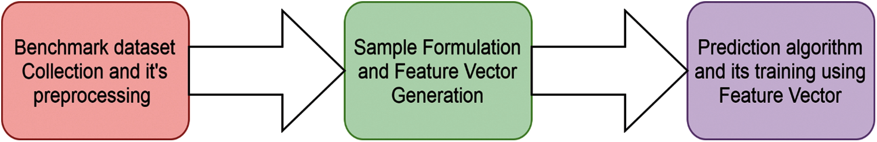
Figure 3: Sequence flowchart
Each qi represents the sequence of alphabetical order of every different amino acid residue frequency.
2.2.4 PRIM as Position Relative Incidence Matrix Generation
20x20 matrix is formed for positional information of residue so that its name is HPRIM. The formula which helps for the calculation is given as
Each
2.2.5 RPRIM as Reverse Position Relative Incidence Matrix Generation
HRPRIM is calculated. It can be calculated by using the formula
It gives us the 400 same coefficients as we received from HPRIM.
2.2.6 Generation of AAPIV as (Accumulation Absolute Positions Incidence Vector)
This contains no relation and no positional information, so the AAPIV was entertained by positional information. By using 20 sequences length, it can be calculated.
2.2.7 Generation of RAAPIV as (Reverse Accumulation Absolute Positions Incidence Vector)
RAAPIV can be calculated with the relation of an informational position to find out hidden and deep features.
A method is used for error detection, which is the back-propagation method. Most feature extractors are available for sequence matrix and consist of PRIM, RPRIM and central raw moments, i.e., RAAPIV, AAPIV, FV, and SVV. FV preserved Relative information of 194 proteins for their positions and representation. Using FV and IFM as input feature matrix is formed, and a Feature vector is represented in each IFM row. OM is formed for every output by applying labels of output from Input Feature Matrix. By using all the above processes, Artificial Neural Network is trained. Input Feature Matrix is used to take input. Output Matrix is used to detect errors by applying back-propagation [25,26], as shown below in Fig. 4.
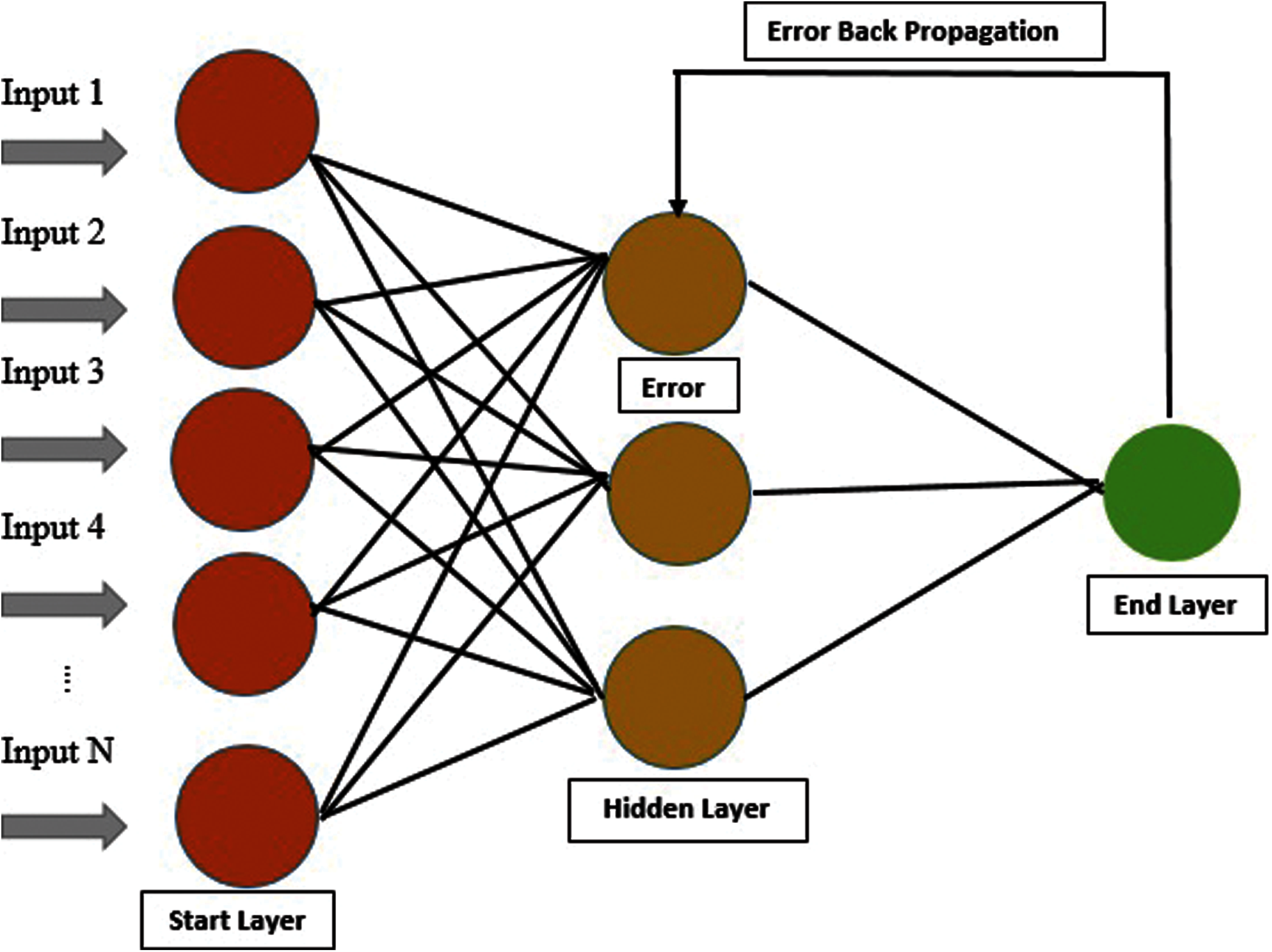
Figure 4: Architecture of ANN of our proposed model
While creating the latest predictor model, it is important to observe and estimate the model’s success rate. To satisfy our evaluation model, two very important questions that we should ask. (1) Which metrics are best for our prediction model quality? (2) What are the test methods that should use for score metrics?
To find out the performance and ACC of the model, there are four types of metrics which mostly helpful for calculation.
I) To find out the overall impact of the model, ACC is used.
II) To find out sensitivity, Sn is used.
III) To find out the specificity of the model, Sp is used.
IV) For stability, we use MCC.
Fortunately, a group of four equations were derived [21,27] is given below in Eq. (13)
Whether this is palmitoylated or non-palmitoylated sites, Eq. (13) explains sensitivity, accuracy, performance and specificity, especially with the help of Mathews Correlation Coefficient. These metrics are mentioned in most of the latest researches [28–30]. There is a separate difficulty for multi-label site prediction, and this is so common in bio and biomedicine [31,32], which require metrics of separate types.
3.3 Predictor Model Validation Process
The metrics of Eq. (13) helps to describe the frequently used validation methods like self-consistency test, independent set test, and k-fold cross-validation test. All of the above tests are considered very important and used for the validation of predictor quality. The new predictor model has been compared with the previous predictors to find out the statistical analysis of the model [33–35].
3.3.1 Self-Model Consistency Testing
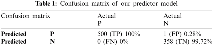
The proposed Computational model is applied for predicted and actual classification, and the results show the values of true positive (TP), false positive (FP), false negative (FN) and true negative (TN). The complete view of predicted and actual model values is displayed in the confusion matrix in Tab. 1.
Another tool shows the predictor model results, which is Receiver Operating Characteristics (ROC). The representation of the self-consistency test of this model is shown in the ROC graph in Fig. 5.
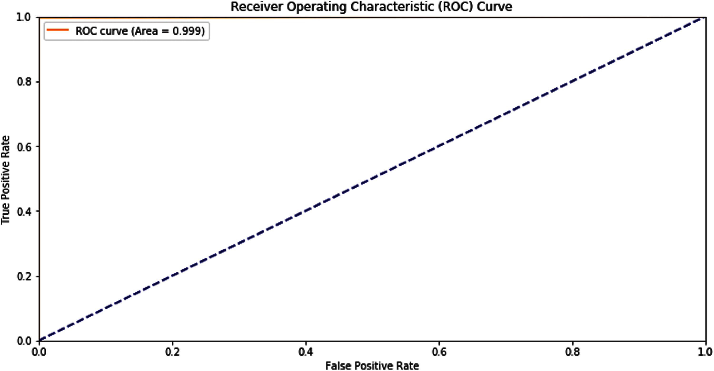
Figure 5: ROC graph of self-consistency
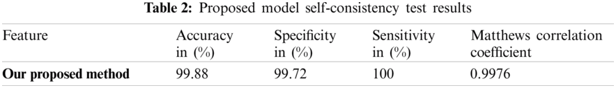
The overall performance of the system can be seen through self-consistency testing Tab. 2.
3.3.2 Ten-Fold Cross-Validation and Testing
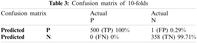
Cross-validation is the process of checking whether the proposed system is perfect and more acceptable in the absence of a validation set. The dataset is divided into k-folds. The proposed Computational model is applied for predicted and actual classification, and the results show the values of true positive (TP), false positive (FP), false negative (FN) and true negative (TN). The complete view of predicted and actual model values is displayed in the confusion matrix in Tab. 3. The overall average accuracies of cross-validation results are shown in Tab. 4.
Receiver Operating Characteristics (ROC) graph of 10-folds of our proposed predictor model is shown below as in Fig. 6.
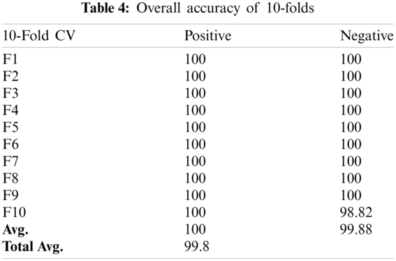
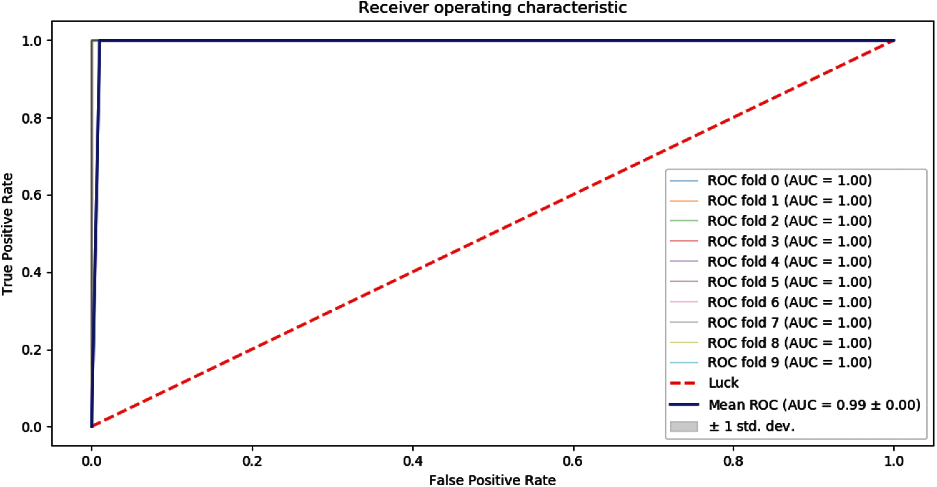
Figure 6: ROC graph of 10-folds cross-validation
Relatively collected datasets are used for the prediction model from previous experiment outcomes. Sometimes it depends upon the current situation to calculate model accuracy by testing using previous data. Still, it is not so easy to get the datasets that are already experimentally proven. It might be possible to get an authentic dataset but insufficient to get the result. In this condition, a specific test is performed to check the model’s credibility. If a validation set is missing, then the cross-validation method is applied to study the model performance. The accumulative dataset results are shown below in Fig. 7.
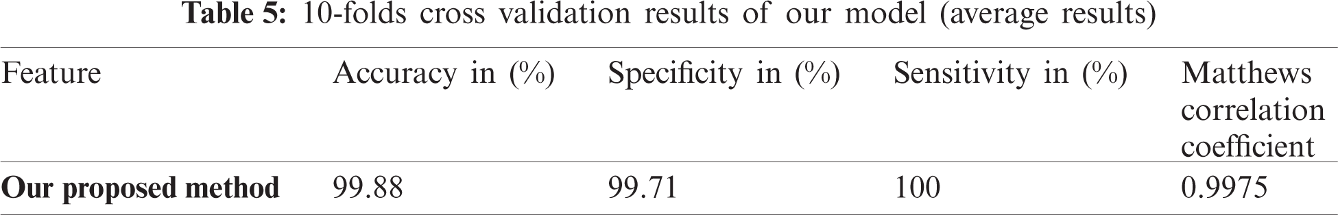
An essential part after training is testing. Testing can be carried out ‘X’ times and can act on every single partition and after that on every iteration, hence result from accuracy can easily measure. Cross-validation is applied for the measurement of the average precision of total results. Another same method is used for positive and negative datasets. Initially, ‘X’ chooses a random value for subsets formation. Cross-validation is used for unbiased data because it is beneficial as compared with the other methods. Results of ten-fold cross-validation are given in Tab. 5.
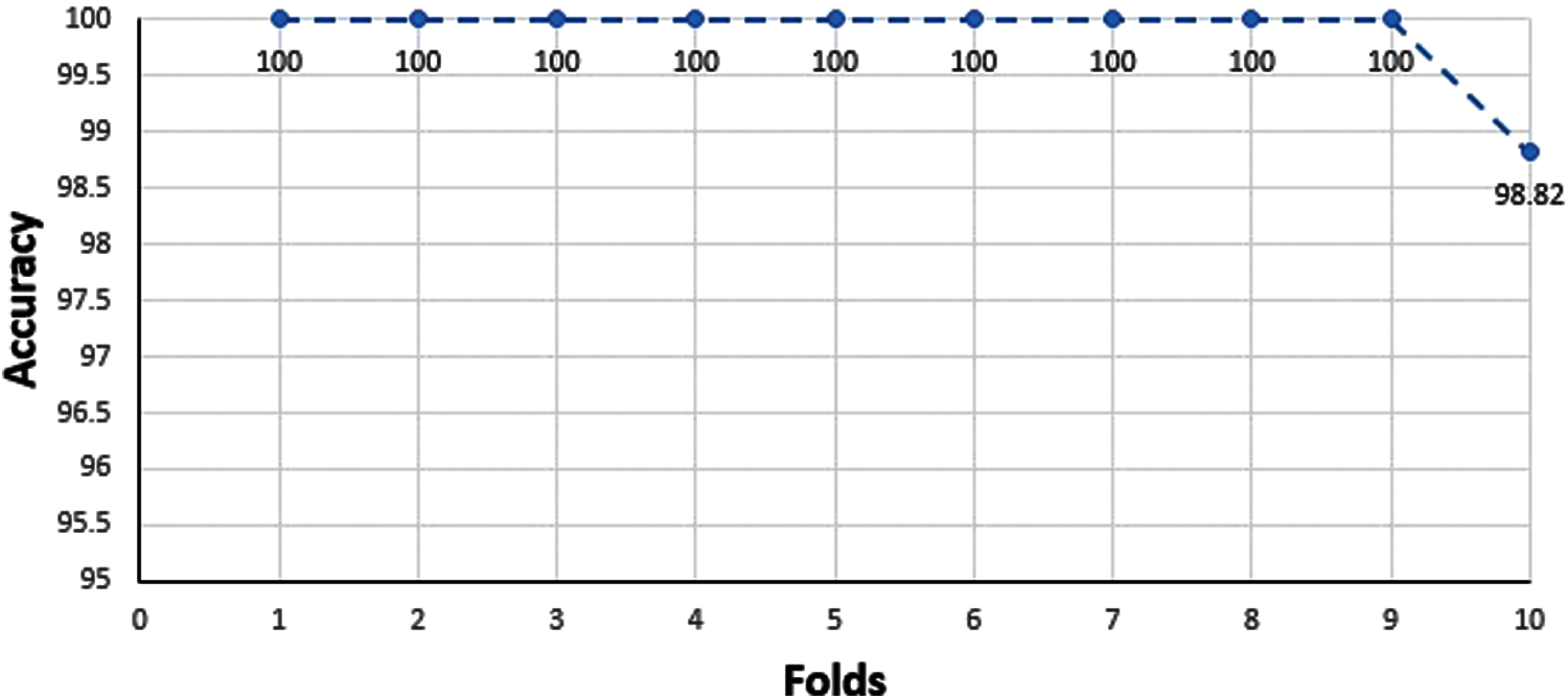
Figure 7: Accumulative dataset results of 10-folds cross-validation
3.3.3 Independent Dataset Testing of Predictor Model
To apply independent dataset testing, we have divided our dataset into two parts. One part is for training, and the other part is for testing. We split 70% dataset for training and used 30% dataset for testing our proposed predictor, and after that, the independent dataset test is executed for lipoylation. The proposed Computational model is applied for predicted and actual classification, and the results show the values of true positive (TP), false positive (FP), false negative (FN) and true negative (TN). The complete view of predicted and actual model values is displayed in the confusion matrix of Tabs. 6 and 7.
Receiver Operating Characteristics (ROC) graph of Independent dataset testing of our proposed predictor model is shown in Fig. 8.

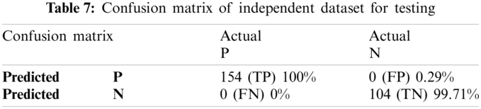
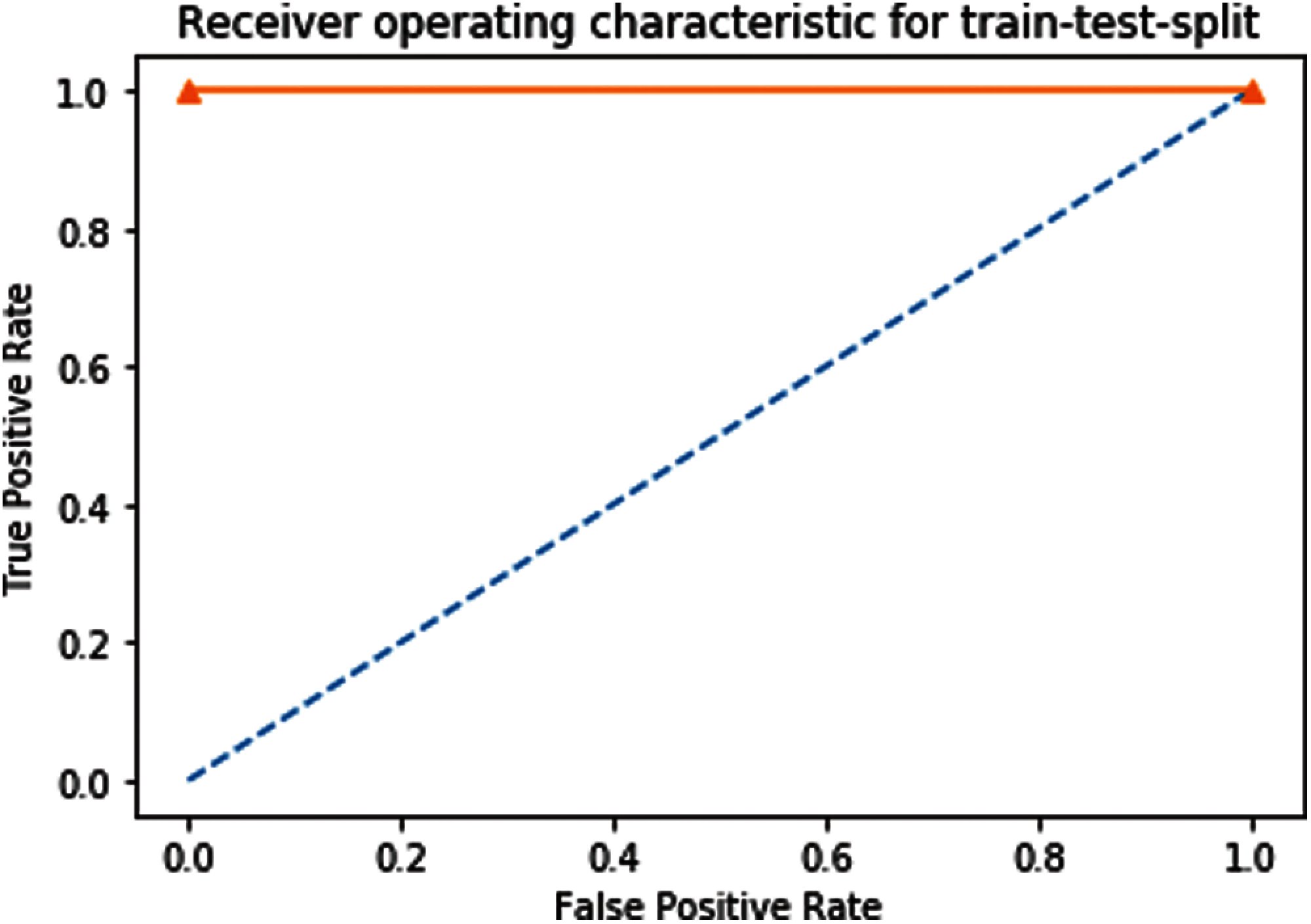
Figure 8: ROC of independent dataset testing
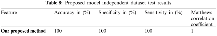
The overall performance of the system can be seen through independent testing. The result of the testing is shown below in Tab. 8.
3.4 Comparison Analysis of Our Proposed Method with Other Feature Methods
To find out the usefulness of our predictor model, we made a comparative analysis with already exist predictors for lipoylation sites. From Tab. 9, we can find out the model comparison with amino acid composition (AAC) [36], KNN Features, Secondary tendency structure, Bi-gram [37], Tri gram [38], amino acid factors (AAF) [39], binary encoding (BE), bi-profile bays feature (BPB) [40] and flexible neural tree (LipoFNT) [41]. These methods are mostly used in computational biology.
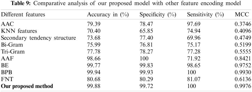
As shown in Tab. 4, our predicted model has achieved 0.9976 as the highest value of MCC by applying Chou’s formulation method and using the ANN algorithm. The other achieved values of our predictor are 99.72% in SP, 99.88% in ACC and 100% in SN, respectively. The final result shows that our feature model is most suitable for predicting lipoylation sites and can get the highest results compared with other predictive models.
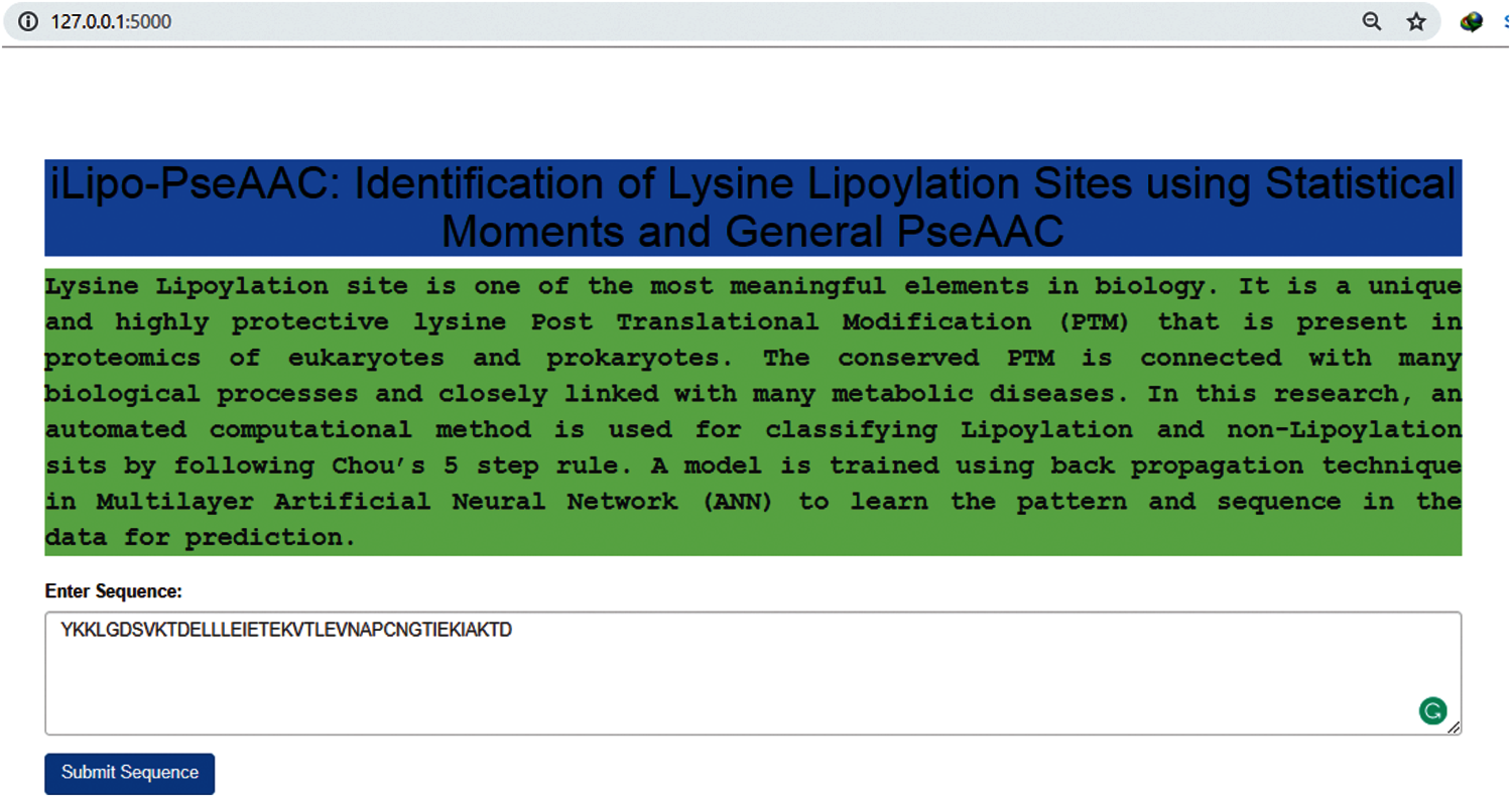
Figure 9: Webserver of our predictor model
As described in most of the latest research papers [42–44], a web server that is publicly available and user friendly shows the direction towards the future development of the model that could help for analysing computational tools and their findings. Specifically, numerous valuable web servers are progressively affecting clinical science, causing an extraordinary transformation in drug science. The webserver is used to fulfil the user requirements online. In our research, the user can open our webserver, put a lipoylation sequence, and press submits to get the result. So, I have made an endless effort to develop a web server for the predictor model, as already discussed in this research. The webserver of our model [45] is given below in Fig. 9.
This research intended to introduce a unique and accurate predictor model to predict lipoylation sites to get the desired results. The model’s performance was checked by applying self-model consistency and ten-fold cross-validation with the help of accuracy metrics. The self-model consistency testing of MCC, Sp, Acc, and Sn results are 0.9976, 99.72%, 99.88%, and 100%, respectively, as shown in Tab. 1. MCC has achieved a maximum value of 0.9975. On the other hand, the predictor achieved the values, i.e., 99.71%, 99.88% and 100% for specificity, accuracy, and sensitivity, respectively. A comparative analysis was made with other predictor models, as shown in Tab. 3. This is indicative that our predictor model can impressively control the situation of the unbalanced problem of lipoylation and can help predict the lipoylation sites in a precise and efficient manner.
Funding Statement: This research was funded by the Deanship of Scientific Research at Princess Nourah bint Abdulrahman University through the Fast-track Research Funding Program.
Conflicts of Interest: The authors declare that they have no conflicts of interest to report regarding the present study.
1. E. A. Rowland, C. K. Snowden and I. M. Cristea, “Protein lipoylation: An evolutionarily conserved metabolic regulator of health and disease,” Current Opinion in Chemical Biology, vol. 42, no. Pt 3, pp. 76–85, 2018. [Google Scholar]
2. M. G. Posner, A. Upadhyay, S. J. Crennell, A. J. A. Watson, S. Dorus et al., “Post-translational modification in the archaea: Structural characterisation of multi-enzyme complex lipoylation,” Biochemical Journal, vol. 449, no. 2, pp. 415–425, 2013. [Google Scholar]
3. J. Collins, T. Zhang, S. W. Oh, R. Maloney and J. Fu, “DNA-crowded enzyme complexes with enhanced activities and stabilities,” Chemical Communications, vol. 53, no. 97, pp. 13059–13062, 2017. [Google Scholar]
4. T. Tietjen and R. G. Wetzel, “Extracellular enzyme-clay mineral complexes: Enzyme adsorption, alteration of enzyme activity, and protection from photodegradation,” Aquatic Ecology, vol. 37, no. 4, pp. 331–339, 2003. [Google Scholar]
5. T. E. McAllister, T. L. Yeh, M. I. Abboud, I. K. H. Leung, E. S. Hookway et al., “Non-competitive cyclic peptides for targeting enzyme-substrate complexes,” Chemical Science, vol. 9, no. 20, pp. 4569–4578, 2018. [Google Scholar]
6. L. J. Reed, “From lipoic acid to multi-enzyme complexes,” Protein Science, vol. 7, no. 1, pp. 220–224, 1998. [Google Scholar]
7. L. J. Reed, “A trail of research from lipoic acid to α-keto acid dehydrogenase complexes,” Journal of Biological Chemistry, vol. 276, no. 42, pp. 38329–38336, 2001. [Google Scholar]
8. J. E. Cronan, X. Zhao and Y. Jiang, “Function, attachment and synthesis of lipoic acid in Escherichia coli,” Advances in Microbial Physiology, vol. 50, no. Pt 8, pp. 103–146, 2005. [Google Scholar]
9. M. D. Spalding and S. T. Prigge, “Lipoic acid metabolism in microbial pathogens,” Microbiology and Molecular Biology Reviews, vol. 74, no. 2, pp. 200–228, 2010. [Google Scholar]
10. C. S. Tsai, M. W. Burgett and L. J. Reed, “α-Keto acid dehydrogenase complexes (xx). A kinetic study of the pyruvate dehydrogenase complex from bovine kidney,” Journal of Biological Chemistry, vol. 248, no. 24, pp. 8348–8352, 1973. [Google Scholar]
11. M. Shabaz and U. Garg, “Predicting future diseases based on existing health status using link prediction,” World Journal of Engineering, In press, pp. 1708–5284, 2021. [Google Scholar]
12. T. I. Baig, T. M. Alam, T. Anjum, S. Naseer, A. Wahab et al., “Classification of human face: Asian and non-asian people,” in Int. Conf. on Innovative Computing (ICICLahore, Pakistan, pp. 1–6, 2019. [Google Scholar]
13. K. C. Chou, “Prediction of signal peptides using scaled window,” Peptides, vol. 22, no. 12, pp. 1973–1979, 2001. [Google Scholar]
14. K. C. Chou and D. W. Elrod, “Bioinformatical analysis of g-protein-coupled receptors,” Journal of Proteome Research, vol. 1, no. 5, pp. 429–433, 2002. [Google Scholar]
15. H. Lin, C. Ding, Q. Song, P. Yang, H. Ding et al., “The prediction of protein structural class using averaged chemical shifts,” Journal of Biomolecular Structure and Dynamics, vol. 29, no. 6, pp. 1147–1153, 2012. [Google Scholar]
16. J. Jia, Z. Liu, X. Xiao, B. Liu and K. C. Chou, “pSuc-Lys: Predict lysine succinylation sites in proteins with PseAAC and ensemble random forest approach,” Journal of Theoretical Biology, vol. 394, pp. 223–230, 2016. [Google Scholar]
17. W. Z. Lin, J. A. Fang, X. Xiao and K. C. Chou, “iDNA-Prot: Identification of DNA binding proteins using random forest with grey model,” PLOS One, vol. 6, no. 9, pp. e24756, 2011. [Google Scholar]
18. Y. D. Cai and K. C. Chou, “Predicting subcellular localisation of proteins in a hybridisation space,” Bioinformatics, vol. 20, no. 7, pp. 1151–1156, 2004. [Google Scholar]
19. K. C. Chou and Y. D. Cai, “Prediction of protease types in a hybridisation space,” Biochemical and Biophysical Research Communications, vol. 339, no. 3, pp. 1015–1020, 2006. [Google Scholar]
20. P. M. Feng, H. Lin and W. Chen, “Identification of antioxidants from sequence information using naive Bayes,” Computational and Mathematical Methods in Medicine, vol. 2013, no. 2, pp. 1–5, 2013. [Google Scholar]
21. P. M. Feng, H. Ding, W. Chen and H. Lin, “Naive bayes classifier with feature selection to identify phage virion proteins,” Computational and Mathematical Methods in Medicine, vol. 2013, no. 2, pp. 1–6, 2013. [Google Scholar]
22. K. C. Chou, “Impacts of bioinformatics to medicinal chemistry,” Medicinal Chemistry, vol. 11, no. 3, pp. 218–234, 2015. [Google Scholar]
23. Y. D. Khan, F. Ahmad and M. W. Anwar, “A neuro-cognitive approach for Iris recognition using back propagation,” World Applied Sciences Journal, vol. 16, no. 5, pp. 678–685, 2012. [Google Scholar]
24. Y. D. Khan, F. Ahmed and S. A. Khan, “Situation recognition using image moments and recurrent neural networks,” Neural Computing and Applications, vol. 24, no. 7–8, pp. 1519–1529, 2014. [Google Scholar]
25. Y. D. Khan, N. Rasool, W. Hussain, S. A. Khan and K. C. Chou, “iPhosT-PseAAC: Identify phosphothreonine sites by incorporating sequence statistical moments into PseAAC,” Analytical Biochemistry, vol. 550, no. 1, pp. 109–116, 2018. [Google Scholar]
26. L. Jiang, J. Zhang, P. Xuan and Q. Zou, “BP neural network could help improve pre-miRNA identification in various species,” BioMed Research International, vol. 2016, no. 12, pp. 1–11, 2016. [Google Scholar]
27. Y. Xu, X. J. Shao, L. Y. Wu, N. Y. Deng and K. C. Chou, “iSNO-AAPair: Incorporating amino acid pairwise coupling into PseAAC for predicting cysteine S-nitrosylation sites in proteins,” PeerJ, vol. 1, pp. e171, 2013. [Google Scholar]
28. M. U. Ghani, T. M. Alam and F. H. Jaskani, “Comparison of classification models for early prediction of breast cancer,” in Int. Conf. on Innovative Computing (ICICLahore, Pakistan, IEEE, 2019. [Google Scholar]
29. Y. Ali, A. Farooq, T. M. Alam, M. S. Farooq, M. J. Awan et al., “Detection of schistosomiasis factors using association rule mining,” IEEE Access, vol. 7, pp. 186108–186114, 2019. [Google Scholar]
30. M. Z. Latif, K. Shaukat, S. Luo, I. A. Hameed, F. Iqbal et al., “Risk factors identification of malignant mesothelioma: A data mining based approach,” in 2020 Int. Conf. on Electrical, Communication, and Computer Engineering (ICECCEIstanbul, Turkey, IEEE, 2020. [Google Scholar]
31. T. M. Alam, M. A. Iqbal, Y. Ali, A. Wahab, S. Ijaz et al., “A model for early prediction of diabetes,” Informatics in Medicine Unlocked, vol. 16, pp. 100204, 2019. [Google Scholar]
32. M. Shabaz and U. Garg, “Shabaz-Urvashi link prediction (SULPA novel approach to predict future friends in a social network,” Journal of Creative Communications, vol. 16, no. 1, pp. 27–44, 2021. [Google Scholar]
33. Y. Xu, X. Wen, X. J. Shao, N. Y. Deng and K. C. Chou, “iHyd-PseAAC: Predicting hydroxyproline and hydroxylysine in proteins by incorporating dipeptide position-specific propensity into pseudo amino acid composition,” International Journal of Molecular Sciences, vol. 15, no. 5, pp. 7594–7610, 2014. [Google Scholar]
34. W. R. Qiu, B. Q. Sun, X. Xiao, Z. C. Xu and K. C. Chou, “iHyd-PseCp: Identify hydroxyproline and hydroxylysine in proteins by incorporating sequence-coupled effects into general PseAAC,” Oncotarget, vol. 7, no. 28, pp. 44310–44321, 2016. [Google Scholar]
35. C. Wu, P. Lu, F. Xu, J. Duan, X. Hua et al., “The prediction models of anaphylactic disease,” Informatics in Medicine Unlocked, vol. 24, pp. 100535, 2021. [Google Scholar]
36. X. B. Zhou, C. Chen, Z. C. Li and X. Y. Zou, “Using chou’s amphiphilic pseudo-amino acid composition and support vector machine for prediction of enzyme subfamily classes,” Journal of Theoretical Biology, vol. 248, no. 3, pp. 546–551, 2007. [Google Scholar]
37. A. Sharma, J. Lyons, A. Dehzangi and K. K. Paliwal, “A feature extraction technique using bi-gram probabilities of position specific scoring matrix for protein fold recognition,” Journal of Theoretical Biology, vol. 320, no. 3, pp. 41–46, 2013. [Google Scholar]
38. K. K. Paliwal, A. Sharma, J. Lyons and A. Dehzangi, “A tri-gram based feature extraction technique using linear probabilities of position specific scoring matrix for protein fold recognition,” IEEE Transactions on NanoBioscience, vol. 13, no. 1, pp. 44–50, 2014. [Google Scholar]
39. Z. Ju and J. J. He, “Prediction of lysine crotonylation sites by incorporating the composition of k-spaced amino acid pairs into chou’s general PseAAC,” Journal of Molecular Graphics and Modelling, vol. 77, pp. 200–204, 2017. [Google Scholar]
40. Z. Ju and S. Y. Wang, “Predicting lysine lipoylation sites using bi-profile bayes feature extraction and fuzzy support vector machine algorithm,” Analytical Biochemistry, vol. 561–562, pp. 11–17, 2018. [Google Scholar]
41. W. Bao, B. Yang, R. Bao and Y. Chen, “LipoFNT: Lipoylation sites identification with flexible neural tree,” Complexity, vol. 2019, no. 12, pp. 9, 2019. [Google Scholar]
42. T. M. Alam, K. Shaukat, M. Mushtaq, Y. Ali, M. Khushi et al., “Corporate bankruptcy prediction: An approach towards better corporate world,” The Computer Journal, vol. 63, no. 5, pp. 0010–4620, 2020. [Google Scholar]
43. T. M. Alam, K. Shaukat, I. A. Hameed, S. Luo, M. U. Sarwar et al., “An investigation of credit card default prediction in the imbalanced datasets,” IEEE Access, vol. 8, pp. 201173–201198, 2020. [Google Scholar]
44. K. Shaukat, T. M. Alam, I. A. Hameed, S. Luo, J. Li et al., “A comprehensive dataset for bibliometric analysis of SARS and coronavirus impact on social sciences,” Data in Brief, vol. 33, no. 7, pp. 106520, 2020. [Google Scholar]
45. T. I. Baig, “ILipo-PseAAC: Identification of lipoylation sites using statistical moments and general PseAAC,” 2020. [Online]. Available: https://ssc.umt.edu.pk/LifeSciences/Our-Research-Project.aspx. [Google Scholar]
 | This work is licensed under a Creative Commons Attribution 4.0 International License, which permits unrestricted use, distribution, and reproduction in any medium, provided the original work is properly cited. |