DOI:10.32604/cmc.2022.022005
| Computers, Materials & Continua DOI:10.32604/cmc.2022.022005 | |
| Article |
Disturbance Evaluation in Power System Based on Machine Learning
1Department of Electrical Engineering, College of Engineering, Jouf University, Sakaka, 72388, Al-Jouf, Saudi Arabia
2Department of Electrical Engineering, College of Engineering, Prince Sattam bin Abdulaziz University, Wadi Addawaser, 11991, Saudi Arabia
3Department of Electrical Engineering, Aswan Faculty of Engineering, Aswan University, Aswan, 81542, Egypt
4Department of Electrical Engineering, University of Engineering and Technology Peshawar, Pakistan
*Corresponding Author: Emad M. Ahmed. Email: emamahmoud@ju.edu.sa
Received: 23 July 2021; Accepted: 24 August 2021
Abstract: The operation complexity of the distribution system increases as a large number of distributed generators (DG) and electric vehicles were introduced, resulting in higher demands for fast online reactive power optimization. In a power system, the characteristic selection criteria for power quality disturbance classification are not universal. The classification effect and efficiency needs to be improved, as does the generalization potential. In order to categorize the quality in the power signal disturbance, this paper proposes a multi-layer severe learning computer auto-encoder to optimize the input weights and extract the characteristics of electric power quality disturbances. Then, a multi-label classification algorithm based on rating is proposed to understand the relationship between the labels and identify the various power quality disturbances. The two algorithms are combined to construct a multi-label classification model based on a multi-level extreme learning machine, and the optimal network structure of the multi-level extreme learning machine as well as the optimal multi-label classification threshold are developed. The proposed method can be used to classify the single and compound power quality disturbances with improved classification effect, reliability, robustness, and anti-noise performance, according to the experimental results. The hamming loss obtained by the proposed algorithm is about 0.17 whereas ML-RBF, SVM and ML-KNN schemes have 0.28, 0.23 and 0.22 respectively at a noise intensity of 20 dB. The average precision obtained by the proposed algorithm 0.85 whereas the ML-RBF, SVM and ML-KNN schemes indicates 0.7, 0.77 and 0.78 respectively.
Keywords: Optimal power flow; optimization algorithm; deep learning; power systems
With the continuous development of the power system and the diversification of power access forms, the power quality is getting worse and worse. At the same time, various electrical equipment has extremely high requirements for power quality standards. Therefore, identifying and classifying the power quality disturbance signals accurately and quickly is a prerequisite for ensuring stable, safe, and efficient operation of the power grid [1–5].
Machine learning has advanced rapidly in the academia and industry in recent years. Its ability to perform complex recognition tasks has been demonstrated by a large increase in recognition rate on many typical recognition tasks. A significant number of academics have flocked to research its hypotheses and applications. Deep learning is being used in a variety of fields to solve some of the problems in this area. Machine learning research has started to appear in the area of regulation [6–11].
Precise power consumption forecasting not only plays a decision-making role in the real-time power dispatching, but also an effective way to ensure the grid stability, solve power deviations, and save the energy. At present, the state is advancing to achieve the power deviation control from demand as the entry point, and the focus of power sales companies is on power consumption forecasting. The real-time and accuracy of the next-time user power consumption forecast is not only one of the realization goals of demand-side management, but also has positive significance for the safe and stable operation of the power system and the improvement of economic benefits. Due to the characteristics of randomness and uncertainty in short-term power consumption of users, the choice of forecasting method and its ability to overcome the randomness directly affect the implementation quality of real-time and accurate power dispatch [12–18].
Because of the rapid growth of large-scale wind farms, wind energy is playing an increasingly important role in domestic and international power markets as a sustainable and cost-effective renewable energy source. Wind's highly unpredictable capacity, on the other hand, can trigger nonlinear characteristics in the wind power, which can have a number of negative consequences for the wind power system's reliability [19–25]. As a result, developing an accurate and efficient power prediction model is needed to preserve the grid's reliability while also improving the equal planning, dispatching, control, and risk assessment capabilities. Many domestic and foreign researchers have performed relevant research and proposed a variety of new viewpoints and methods, which can be broadly divided into two categories: physical statistics and time series methods. The wind farm's actual physical meteorological data, for example, is used in the physical statistics scheme, which necessitates a large number of parameters, time-consuming calculations, and generally low accuracy [26,27].
With the use of a large number of nonlinear and unbalanced loads in the power system, the impact of power quality on the safe and stable operation of the power system has become more obvious. The real-time and effective classification of power quality disturbances has become the basis for further improvement of power quality. In recent years, the classification of power quality disturbances has been well studied [28–32]: Support vector machine (SVM) method can be used to detect the complex power quality problems. Using multi-label K-nearest neighbor method (ML-KNN), it can clearly detect, locate and classify different power quality problems. The use of multi-label radial basis function neural network (ML-RBF) can improve the classification efficiency and accuracy of common power quality disturbances.
In the field of quality disturbance classification, commonly used feature extraction algorithms include Fourier transform [33], wavelet transform [34], S transform [35,36], Hilbert yellow transform [37,38], etc. Commonly used classification and recognition algorithms include extreme learning machine [8], support vector machine [39], BP neural network [40] and so on. Reference [41] uses the S transform to extract the characteristics of power quality disturbance signals, and recognizes them through GAP-RBF neural network. This method has a small number of neurons and fast calculation speed, but the recognition rate needs to be improved. Reference [42] uses Lagrangian delay to optimize the wavelet basis to extract the power quality disturbance signal features, and uses the probabilistic neural network based on K-means clustering to achieve the classification, but its algorithm needs to extract more features, which leads to feature redundancy. Reference [43] uses a compressed sensing sparse vectors to extract the characteristics of power quality disturbance signals, using neural network performs classification. This method reduces the amount of data that needs to be processed, but the anti-noise performance is not strong. The study found that the existing power quality disturbance classification method lacks a unified classification standard and is prone to redundant features, which leads to a decline in classification accuracy, poor generalization ability, and greater noise.
The above algorithms require feature selection of the signal, which is prone to feature redundancy, and some other features will be lost, resulting in a decrease in recognition rate and reduced anti-noise performance. In order to avoid the process of selecting power quality disturbance features, literature [44,45] converts the power quality disturbance signal into a two-dimensional gray image, and then uses a two-dimensional CNN for image recognition, but the conversion process is complicated, and the grayscale is temporarily reduced and interrupted. The degree of image features is not obvious, resulting in a decline in the recognition rate. For sequence signals such as power quality disturbances, one-dimensional CNN can be used to speed up the calculation. Reference [46] uses the segmented improvement of the S transform to process the time domain resolution and the frequency domain resolution in segments. By analyzing the modulated time-frequency matrix obtained by the improved S transform, the characteristic curve that can reflect the different mutation parameters of the disturbance signal is drawn. The radial basis function neural network of local approximation is used to classify the disturbance signal, but it is difficult to extract the feature quantity under the compound disturbance, and the generality is poor. Reference [47] uses a sparse autoencoder to perform unsupervised learning of the original disturbance signal, which automatically extracts the sparse expression of the disturbance signal data characteristics, and uses the classifier for training to obtain the classification accuracy of various disturbance signals, which solves the shortcoming of the traditional neural network initial randomness of the weight value, but the coding process is complicated.
Power quality disturbance classification in distribution networks is one of the important aspect which is in the focus of both academia and industry. Various methods have been proposed but their classification efficiency is lower. In order to improve the classification efficiency and improve the power quality, this paper focuses on the improvement of classification accuracy and efficiency as the research goal, and proposed a multi-layer extreme learning machine self-encoding network structure, and ranking-based power quality disturbance classification model, and compares it with other classification methods on power quality disturbance classification. The comparison verifies the effectiveness of the proposed method.
The remaining of the paper is organized as follows. In Section 2, the system model is described. In Section 3, the numerical results are provided in detail. Section 4 provides the application scenario while Section 5 concludes the paper.
Multi-layer extreme learning machine based on self-encoding, which can effectively represent the complex functions, has high prediction accuracy and generalization ability. The ranking-based multi-label classification algorithm, taking into account the correlation between the labels, is suitable for the classification of various power quality disturbances, and has a strong anti-noise ability. This paper combines the multi-layer extreme learning machine with the multi-label classification algorithm, and proposes a multi-label classification model based on the multi-layer extreme learning machine.
The extreme learning machine autoencoder (ELM-AE) optimizes the input weight, improves the classification accuracy and generalization ability, overcomes the problem of neuron invalidity caused by the random weight and hidden layer threshold of the extreme learning machine, and improves the classification efficiency [48–50].
The network structure of the extreme learning machine autoencoder is shown in Fig. 1. The number of nodes in the input layer and output layer is n, and the number of nodes in the hidden layer is l.
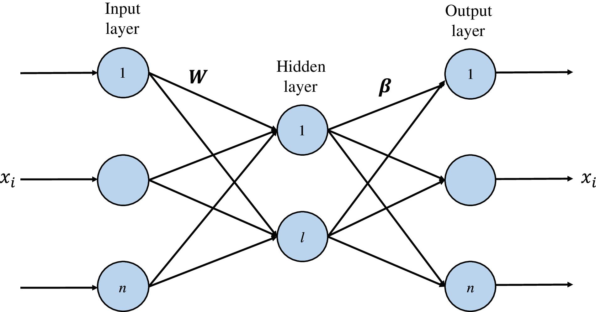
Figure 1: ELM-AE architecture
Suppose there is an arbitrary sample space
Introduce the orthogonal random weight matrix
where
where
By reconstructing the matrix
where
The
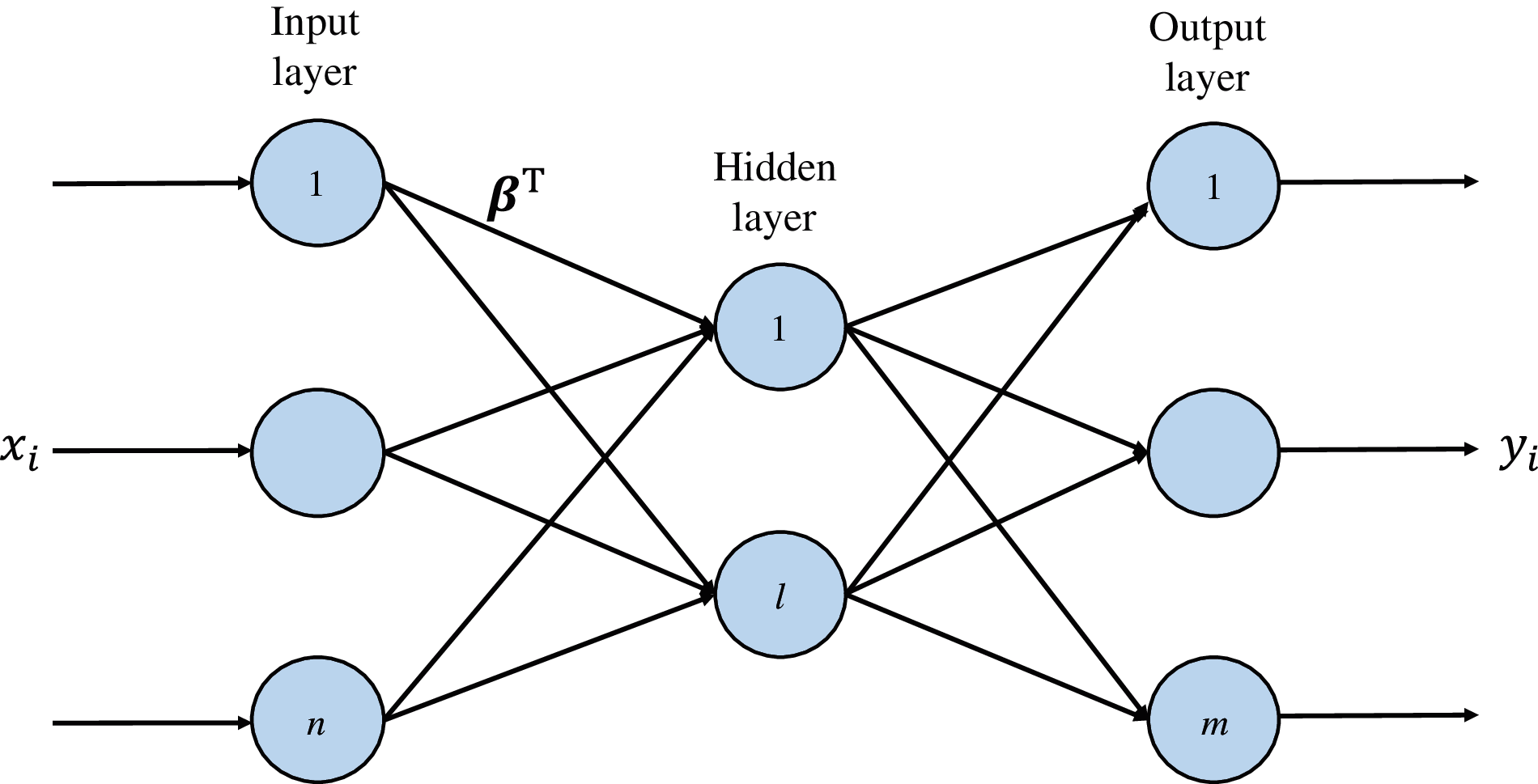
Figure 2: ELM-AE reconfiguration
The multi-layer extreme learning machine autoencoder (ML-ELM-AE) performs stacking operations on the basis of ELM-AE [38,51], and builds a network structure with multiple hidden layers, as shown in Fig. 3, which can improve the average power accuracy and generalization ability of the quality disturbance classification [39,52–57].
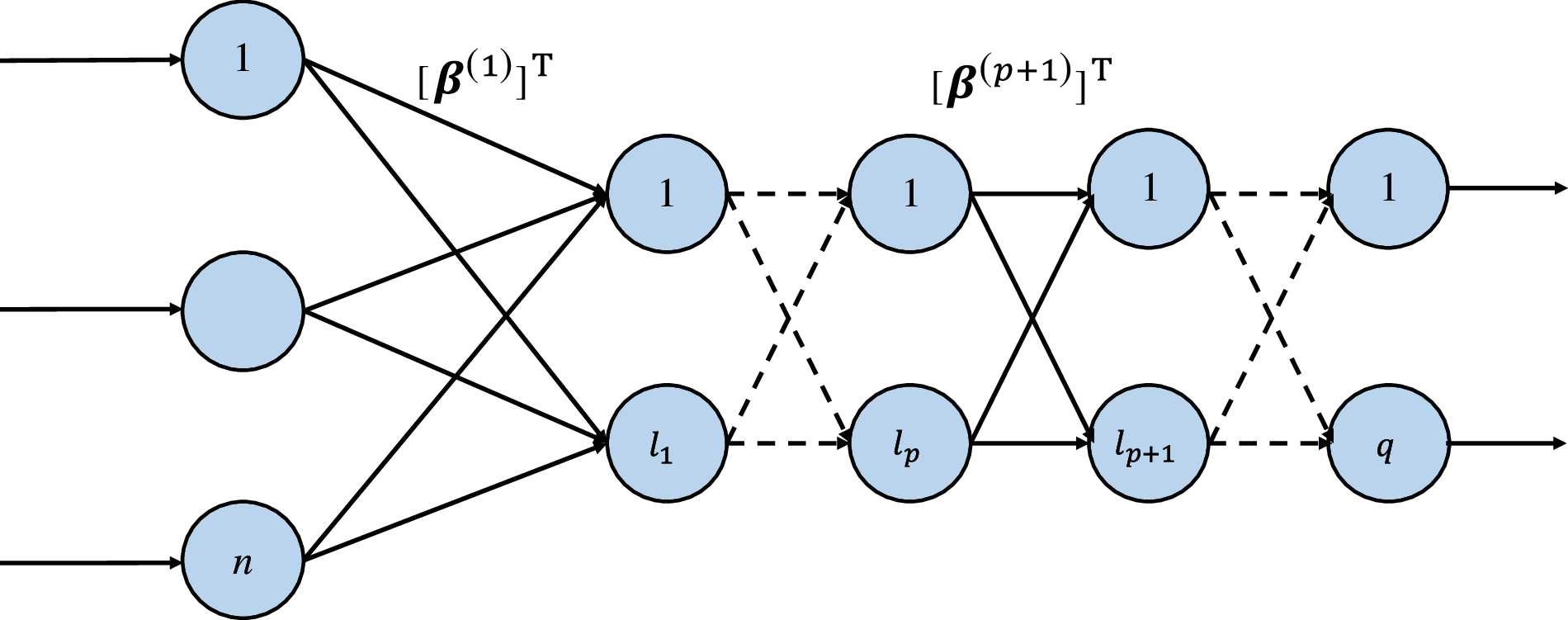
Figure 3: ML-ELM-AE architecture
The first step is to use the set of input data samples to calculate the output matrix
In the second step,
The third step, and so on, takes the output matrix
2.2 Multi-Label Classification Algorithm
In multi-label classification algorithm, a single data sample belongs to the multiple category labels, and fully considering the correlation between the labels [40–42]. This paper uses the ranked classification method to complete the multi-label classification problem.
Assuming that the sample space is S, each sample is a d-dimensional feature vector, namely
Based on the rank-based multi-label classification algorithm [43], a mapping
For the sample
It can be observed that the predicted label set of the sample
Evaluation indicators to measure the effect of multi-label classification algorithms [45,46] mainly include Hamming loss, first-class errors, ranking loss, coverage and average accuracy.
Hamming loss
where n represents the number of samples; L represents the total number of labels;
A one type of error
where
The ranking loss
where
The coverage rate
The average accuracy
where
2.3 Multi-Label Classification Model Based on ML-ELM
In this paper, the self-encoding structure of the multi-layer extreme learning machine and the ranking-based multi-label classification algorithm are combined to construct the basic structure of the classifier model as shown in Fig. 4 [47].
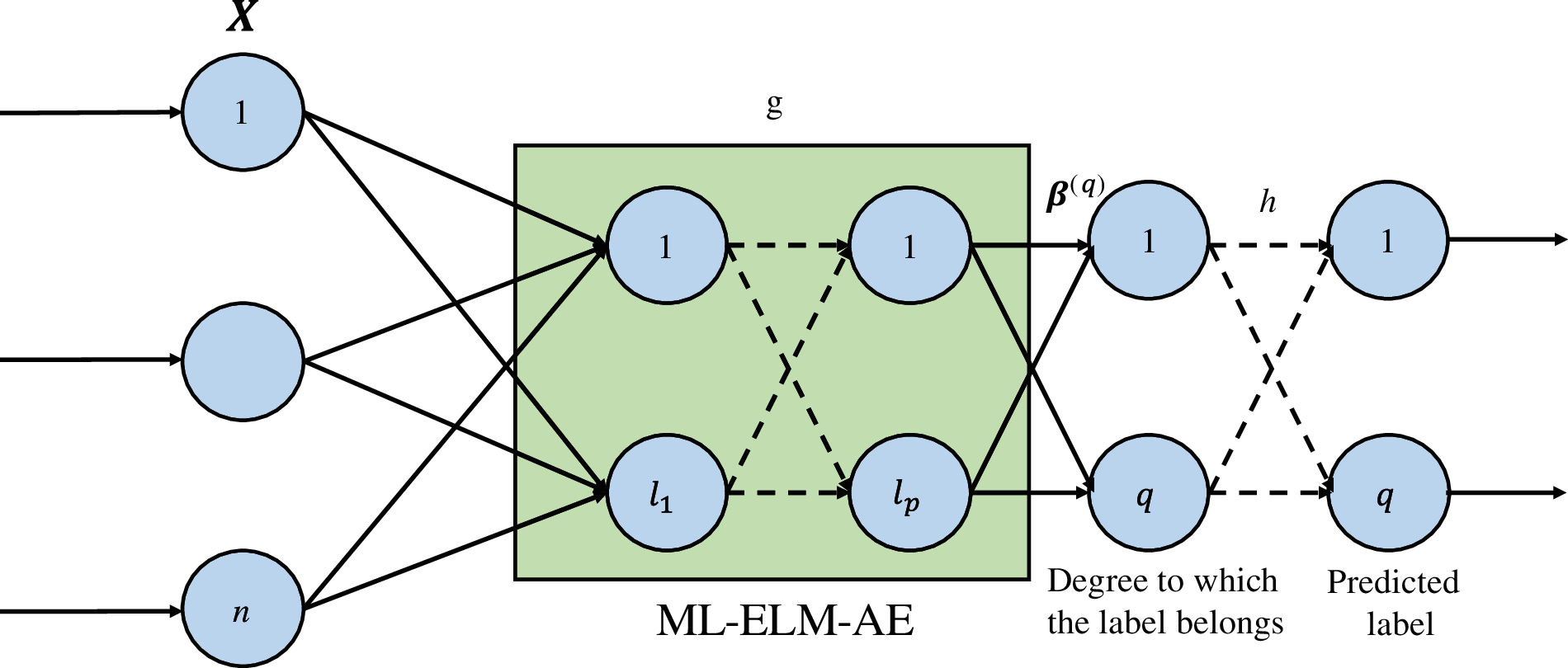
Figure 4: Proposed classifier model
According to the model in Fig. 4, the input sample data is mapped to the label through the ML-ELM-AE network, and then the classification result is obtained through the conversion of the classification function [48]. Among them,
where
In the process of classifying the power quality disturbances, the ML-ELMAE algorithm determines the optimal network structure through experiments based on the set of input data samples, and generates the output matrix and weight matrix of each hidden layer. The ranking-based multi-label classification algorithm determines the optimal classification threshold through experiments [49], and normalizes the classification threshold to (0,1). Combining the two algorithms, a multi-label classification algorithm of multi-layer extreme learning machine is designed, which is suitable for the classification of single disturbance of power quality and the classification of compound disturbances. It has good anti-noise ability and high classification accuracy [50], and overcomes the randomness of traditional ELM parameter assignment, and has high classification efficiency, good robustness and generalization ability.
3 Experimental Results and Analysis
This paper uses the MATLAB simulator to compute the simulation experiment, using average accuracy, hamming loss, first-class error, ranking loss, and coverage as the evaluation indicators of the classification effect. In addition, the experiment also increases the training time and test time of the classifier as a measure of classification efficiency evaluation index. In order to reduce the error, each experimental data is the arithmetic mean of the algorithm program running 20 times under the same experimental conditions.
3.1 Power Quality Disturbance Signal Model
The common single power quality disturbance signal model [51] is shown in Tab. 1, where the fundamental frequency
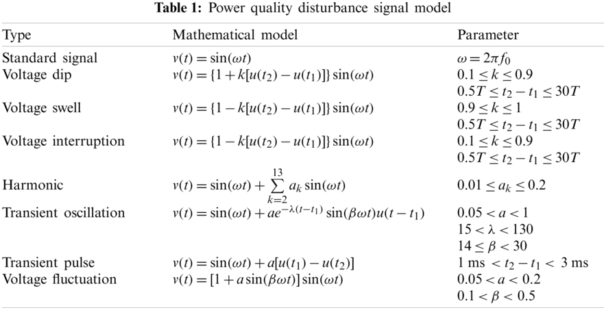
The signal in the experiment is sampled with 3200 Hz as the sampling frequency, 30 cycles are sampled in total, and the total number of sampling points is 1921. All signals are randomly generated 200 samples according to the mathematical model, 100 are used as training data, and the other 100 are used as test data. The training data set and the test data set each contain 4800 samples.
3.2 Classifier Model Parameter Design
In this paper, the optimal network structure of ML-ELM-AE is evaluated through experiments, and the multi-label mapping function
3.2.1 Determination of ML-ELM-AE Network Structure
In this paper, the number of hidden layers of ML-ELM-AE is limited to 9 layers, the number of nodes in each layer is set to 50∼2000, and the number of nodes is changed by 50. The Hamming loss is used as the basis for the evaluation of the classification effect, and the training time and the test time are referred to at the same time, and the network structure parameters of the multi-layer extreme learning machine with good classification effect and high efficiency are selected.
In order to obtain the optimal number of nodes in each layer when the total number of layers is different, the following experimental steps are designed:
1) Set the number of hidden layers of ML-ELM-AE to 1.
2) Set the number of hidden layer nodes to change according to the law of 50 + L × 50 (L is an integer increasing from 0 to 39), get the Hamming loss corresponding to each L value, training time and test time, and select the optimal L value, that is, the optimal number of nodes in this layer is 50 + L × 50.
3) Set the number of layers of ML-ELM-AE to 2, where the number of nodes in the first layer has been fixed by steps 1 and 2, repeat step 2, get the optimal L value of the second layer, and get the optimal number of nodes in this layer.
4) Set the number of layers of ML-ELM-AE to 3∼9 in turn, and get the optimal number of nodes for each layer.
Tab. 2 shows the number of nodes in each layer corresponding to the optimal value of Hamming loss when the total number of layers in ML-ELM-AE is 1–9. It can be found that starting from layer 4, the optimal number of nodes for the new hidden layer is 750.
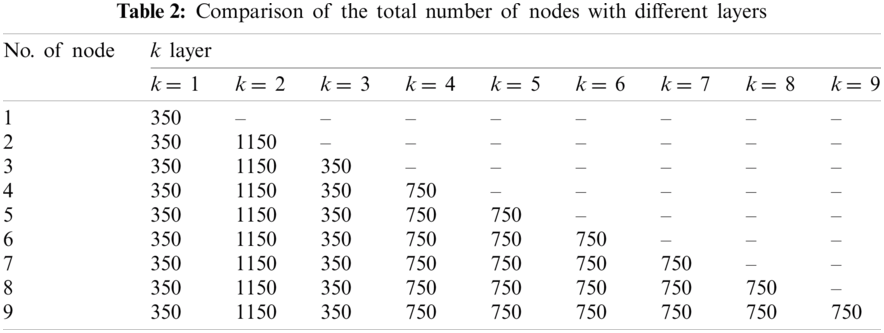
Fig. 5 shows the relationship between the number of hidden layers of ML-ELM-AE and the Hamming loss. It can be found that, the Hamming loss shows a pattern of first decreasing and then tending to be stable. When the number of hidden layers exceeds 4, the Hamming loss is lower.
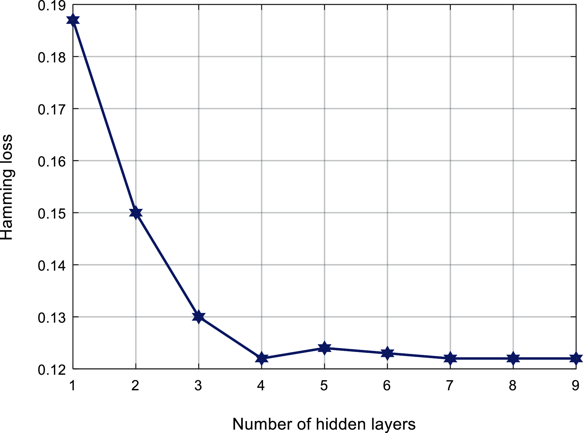
Figure 5: Loss comparison with number of hidden layers
Figs. 6 and 7 respectively shows the relationship between the number of hidden layers of ML-ELM-AE and the training time and test time. It can be found that with the increase of the number of hidden layers, the overall training time and test time shows an increasing trend.
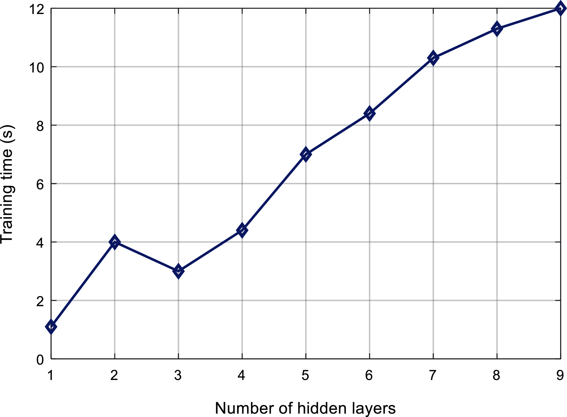
Figure 6: Comparison of training time of the proposed algorithm
Based on the above experimental results, we can observe that, there is not a single quantitative relationship between the number of hidden layers and the number of nodes in ML-ELM-AE and the classification results. There is an optimal number of hidden layers and nodes, which saves training and testing time while ensuring the classification effect and improved efficiency. In this paper, when the number of hidden layers of ML-ELM-AE is 4, the power quality disturbance classification effect is the best and the efficiency is higher. Therefore, this paper sets the multi-layer extreme learning machine as “input layer-hidden layer (350-1150-350-75)” structure of the output layer.
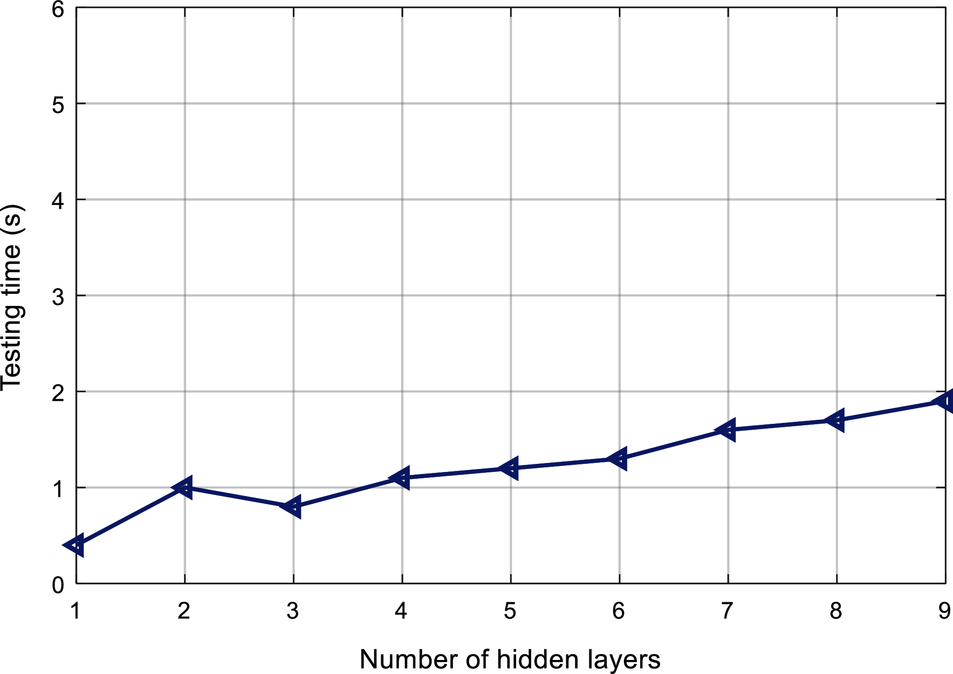
Figure 7: Comparison of testing time of the proposed algorithm
3.2.2 Determination of Classification Threshold
The experiment adopts the optimal 4-layer ML-ELM-AE network structure, and the classification threshold of the multi-label classifier is set in the range of 0.05 to 0.95, with 0.05 as the step interval. The Hamming loss, ranking loss, first-class error, coverage rate, and average accuracy are used as the evaluation basis for the classification effect. Fig. 8 shows the relationship between the classification threshold and the Hamming loss. It can be found that, with the increase of the classification threshold, the Hamming loss quickly decreases and stabilizes, and then slightly increases. When the classification threshold changes around 0.55, the Hamming loss value is smaller.
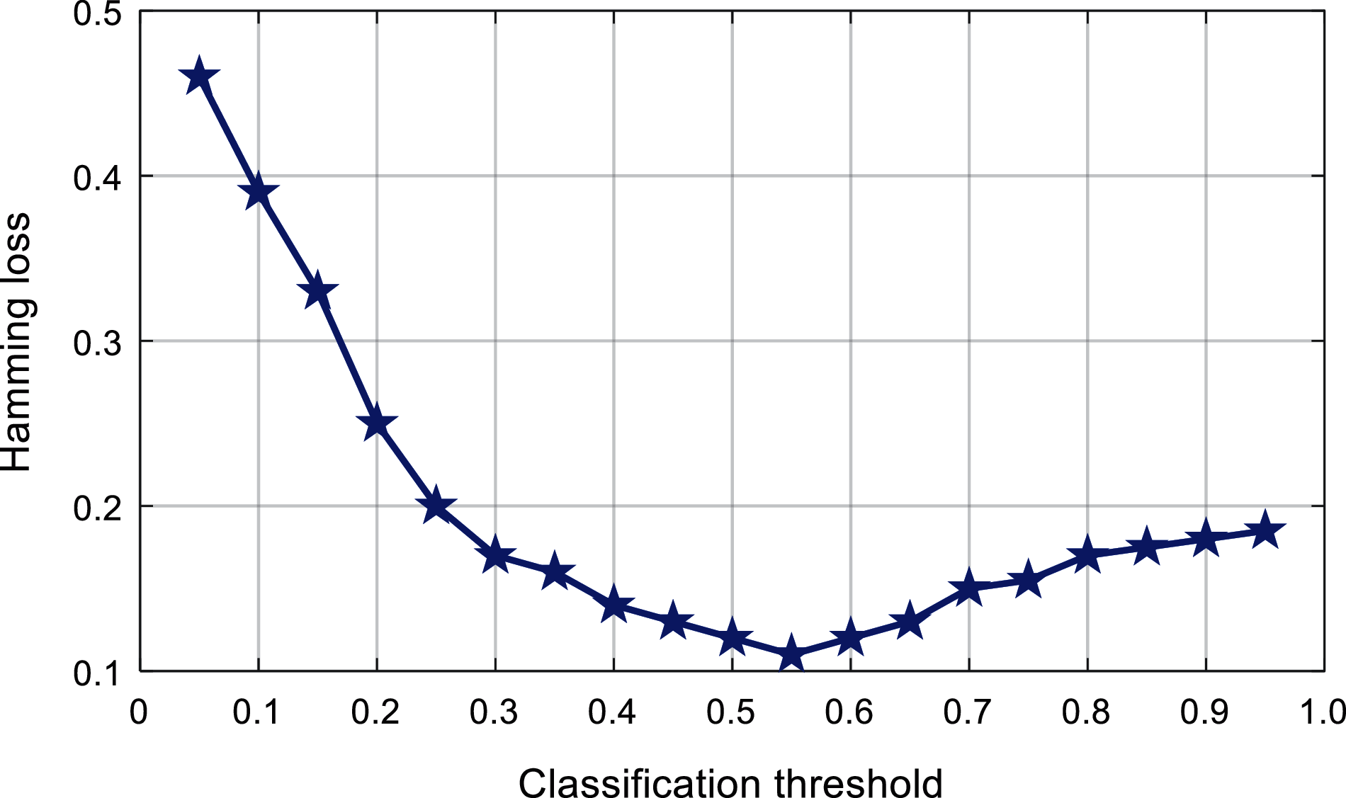
Figure 8: Comparison of the classification threshold of the proposed algorithm
Figs. 9 and 10 respectively shows the relationship between the classification threshold and the one-type of error and the ranking loss. It can be found that the change of the classification threshold has little effect on these two evaluation indicators, and the first type of error in Fig. 9 is floating around 0.086. The ranking loss in Fig. 10 fluctuates around 0.063, and the range of change is small.
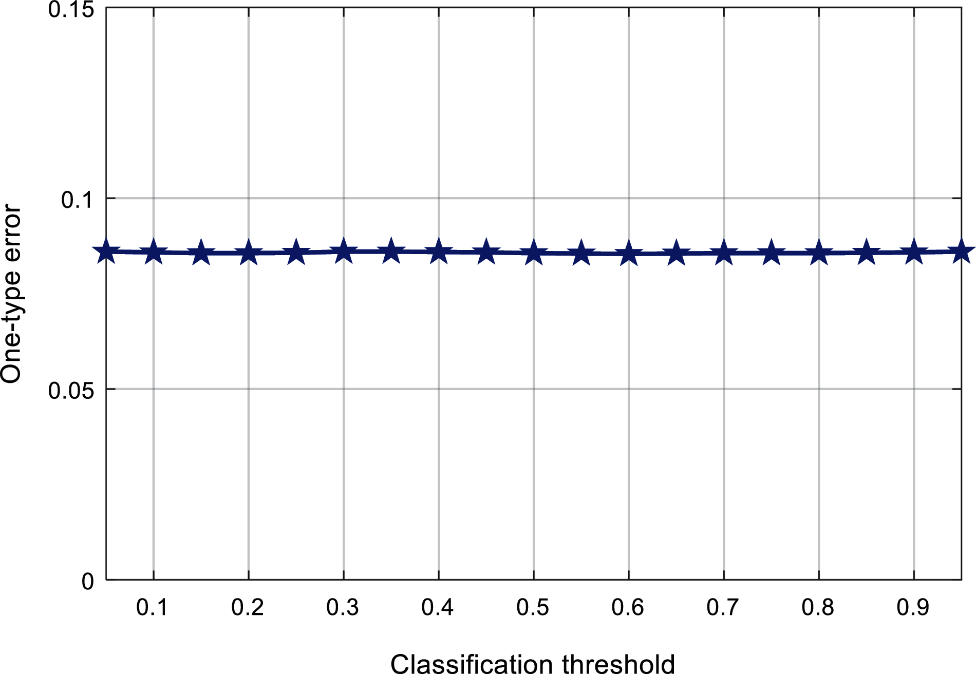
Figure 9: Comparison classification value against the one-type error
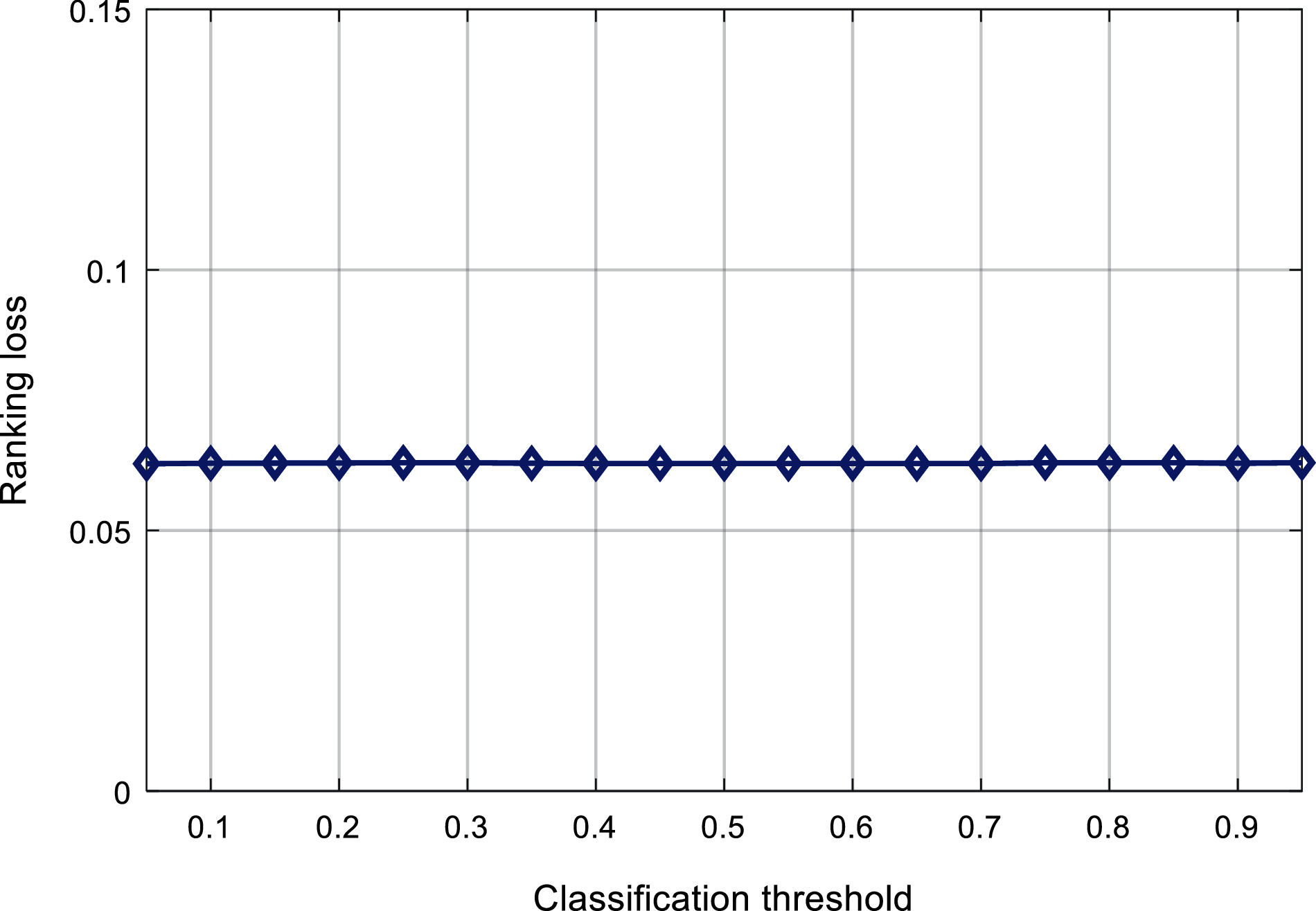
Figure 10: Comparison of classification threshold against ranking loss
Fig. 11 shows the relationship between the classification threshold and the coverage rate. It can be found that, with the change of the classification threshold, the coverage rate fluctuates between 2.006 and 2.017. When the classification threshold is around 0.6, the coverage rate is smaller.
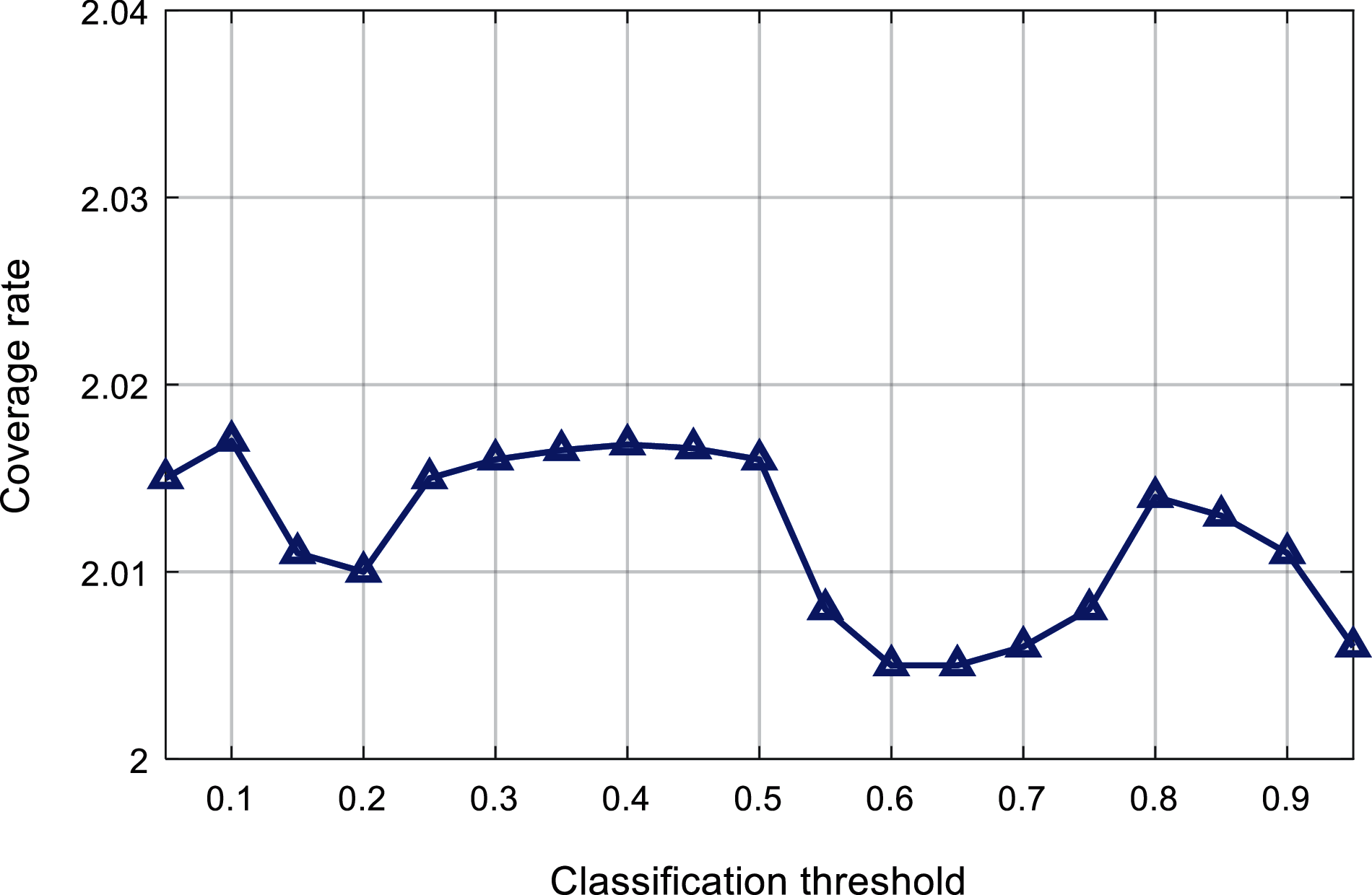
Figure 11: Comparison of classification threshold and coverage
Fig. 12 shows the relationship between the classification threshold and the average accuracy. It can be found that the average accuracy value varies from 0.9075 to 0.9085. When the classification threshold changes around 0.65, the average accuracy value is higher.
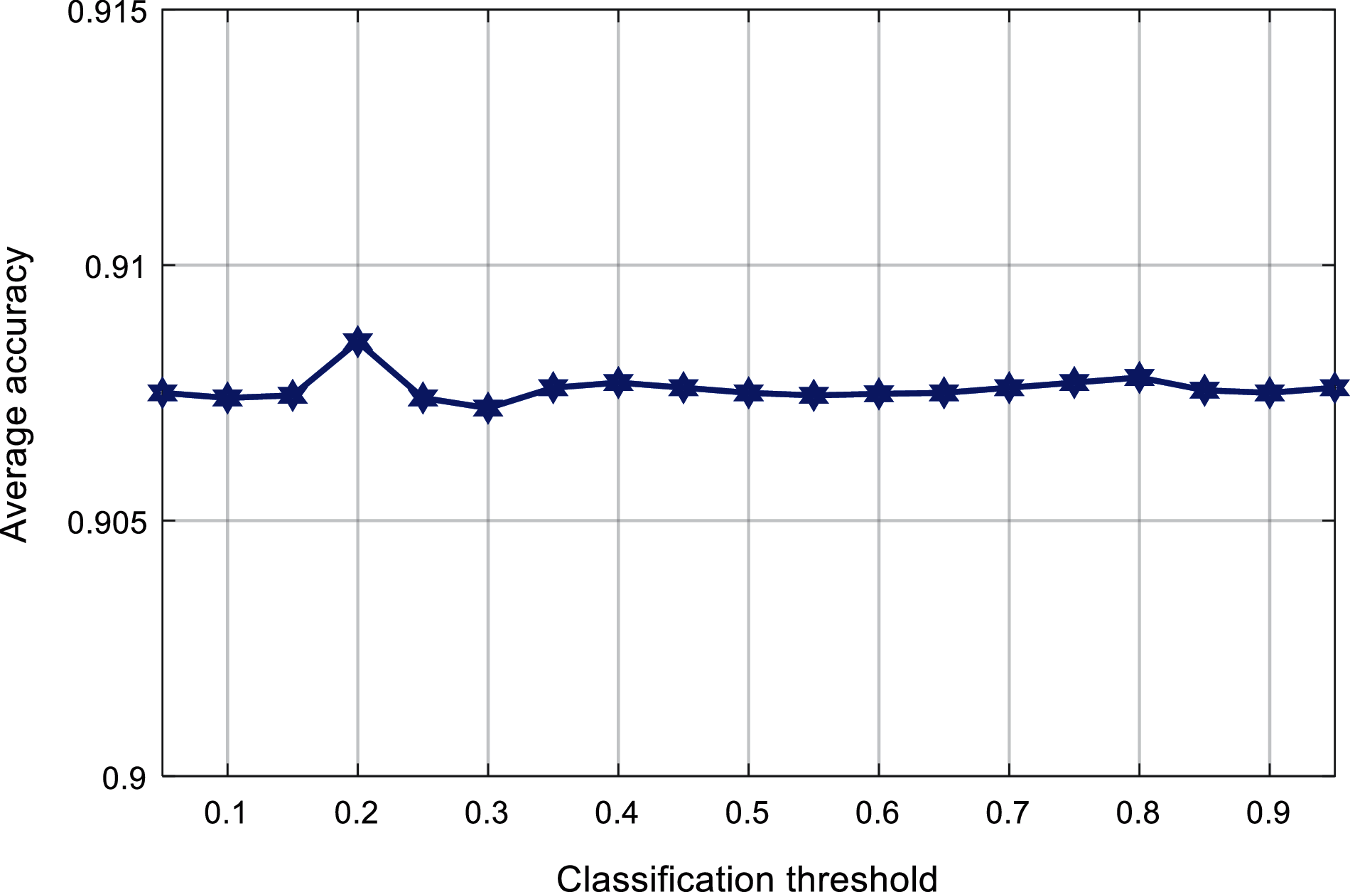
Figure 12: Comparison of classification threshold and average accuracy
Based on the above experimental results, it can be obtained that the classification threshold has a more obvious impact on the Hamming loss, the coverage rate and average accuracy are affected by the change of the classification threshold to a certain extent, and the first type of errors and ranking errors are not significantly affected by the classification threshold. In this paper, the classification threshold of the multi-label classifier is set to 0.6.
3.3 Classification of Experiment Results and Comparison
The multi-label classification model of the multi-layer extreme learning machine is deployed to predict the disturbance category contained in the power quality disturbance signal [54,55].
In the first step, the power quality disturbance signal is subjected to discrete wavelet transform (DWT) to obtain the decomposition coefficients of each layer, and the decomposition coefficients are divided into training data sets and test data sets.
The second step is to randomly generate the weights of each layer of the orthogonalized ML-ELM-AE network.
The third step is to train the multi-layer extreme learning machine network with the training data set as input, and adjust the weights of each layer of the network.
The fourth step is to obtain the classification function of the multi-label classification algorithm according to the mapping relationship of ML-ELM-AE.
Finally, the test data set is used as input, and the multi-label classification model of the trained multi-layer extreme learning machine is used to predict the disturbance category.
3.3.2 Experimental Results and Comparison
The experimental research objects are a single disturbance signal and a composite disturbance signal, and noise disturbances with a signal-to-noise ratio (SNR) of 50, 40, 30 and 20 dB are superimposed on each power quality disturbance signal. The experimental data is the average of the experimental results of various disturbance signals under the same noise intensity. In order to further verify the performance of the power quality disturbance classification method proposed in this paper, the SVM, ML-KNN and MLRBF schemes are used to complete the disturbance signal classification, and the results are compared with the method proposed in this paper.
Tab. 3 shows the Hamming loss of the classification results of various interference signals under different noise levels. Fig. 13 shows the comparison results of the Hamming loss of different classification algorithms. It can be found that the noise intensity is reduced from 50 to 20 dB. Although the Hamming loss value shows an increasing trend, it is lower than the other existing three algorithms.
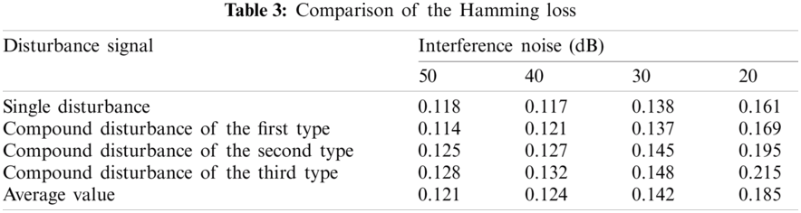
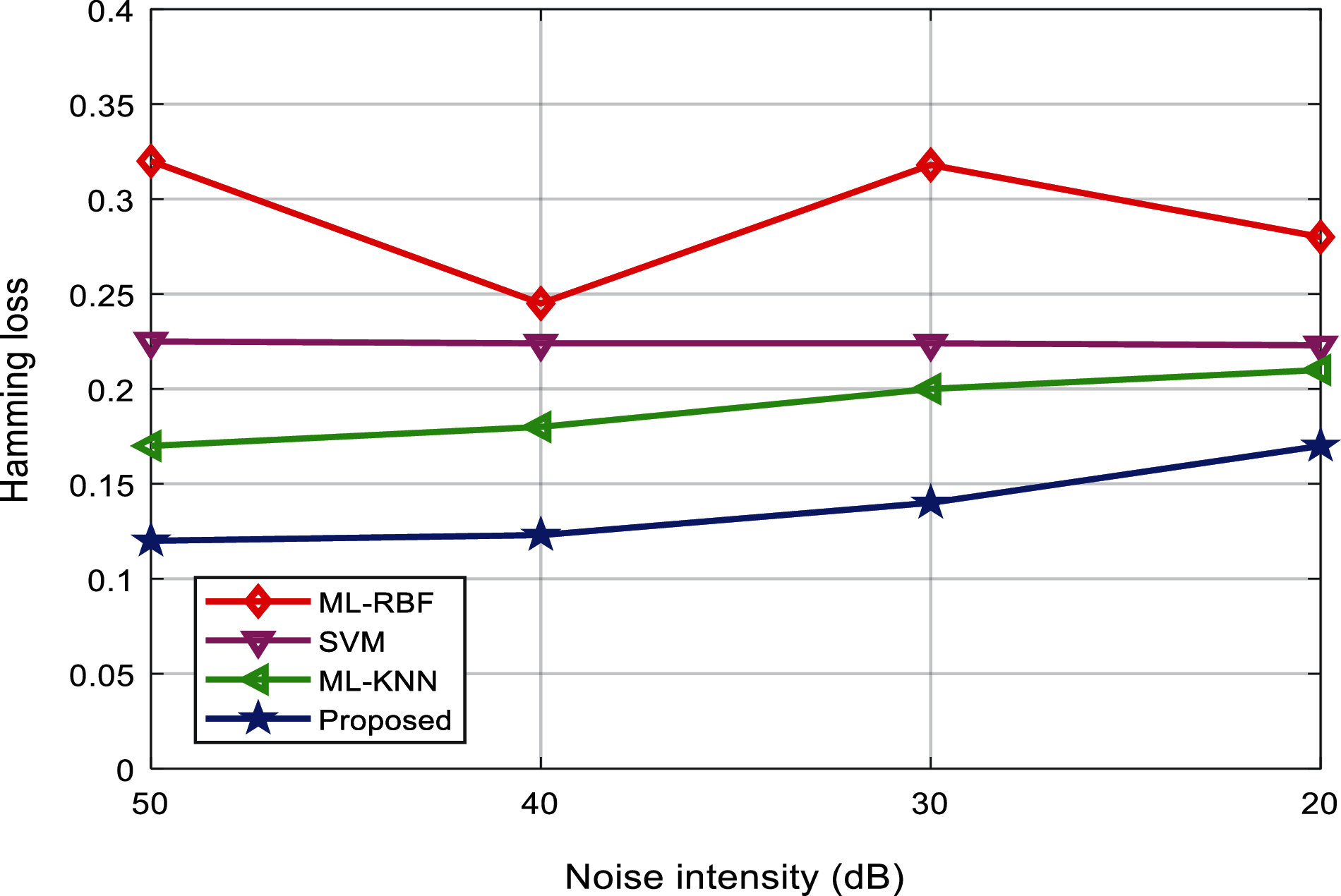
Figure 13: Hamming loss evaluation of the algorithms
Tab. 4 shows the first-class errors of the classification results of various interference signals under different noise levels. Fig. 14 shows the comparison results of the one-type errors of different classification methods. It can be found that the first-class error values of the proposed method are the lowest, and the experimental results under different environments are not much different.
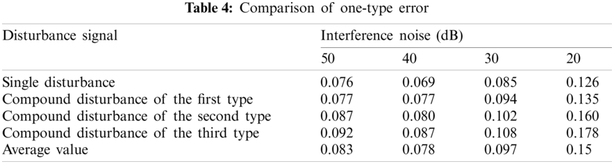
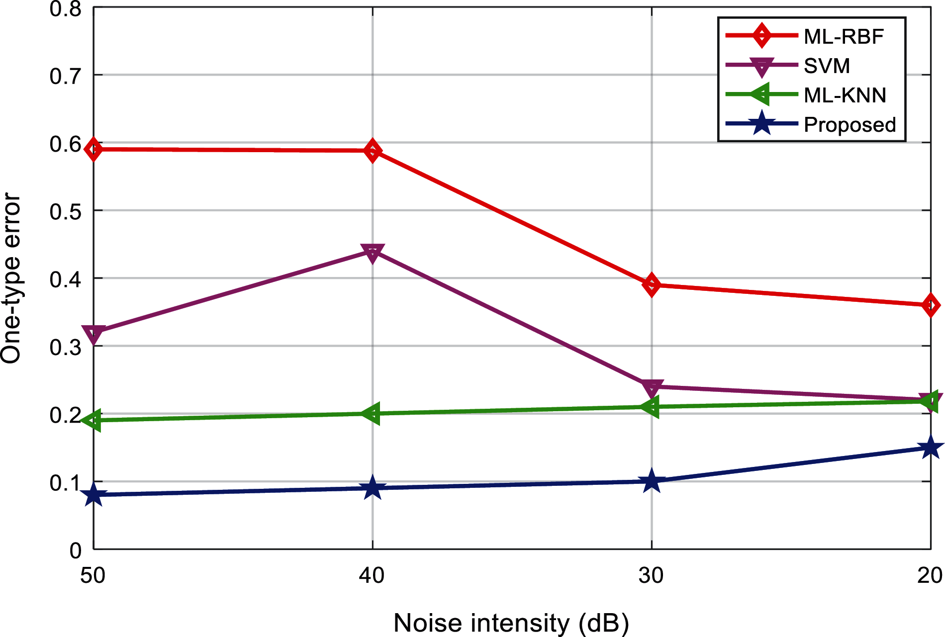
Figure 14: Comparison of one-type error of the algorithms
Tabs. 5 and 6 show the ranking loss and coverage rate of various interference signal classification results under different noise levels. Figs. 15 and 16 show the ranking loss and coverage rate comparison results of different classification methods. It can be found that, the ranking loss value and coverage rate of the proposed method are lower than the other three methods.
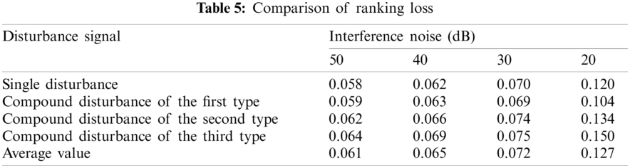
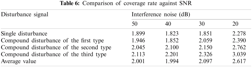
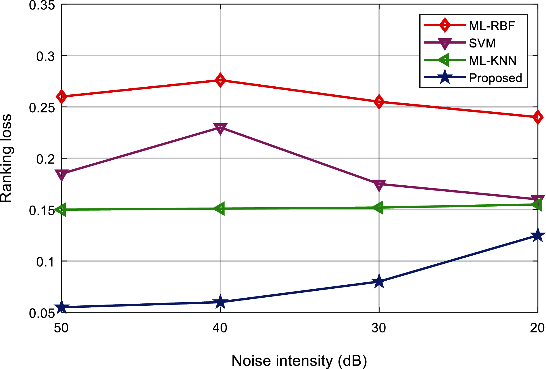
Figure 15: Comparison of ranking loss of the algorithms
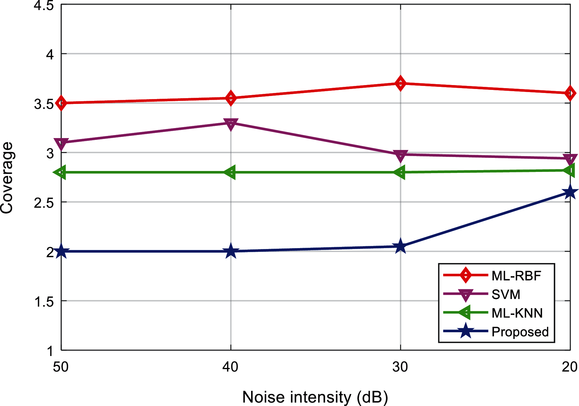
Figure 16: Comparison of coverage of the algorithms
Tab. 7 shows the average accuracy of the classification results of various interference signals under different noise levels. Fig. 17 shows the comparison results of the average accuracy of different classification methods. It can be found that as the interference intensity weakens, the average accuracy of the proposed method shows a downward trend, but higher than the other three methods.
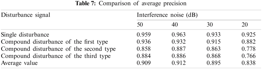
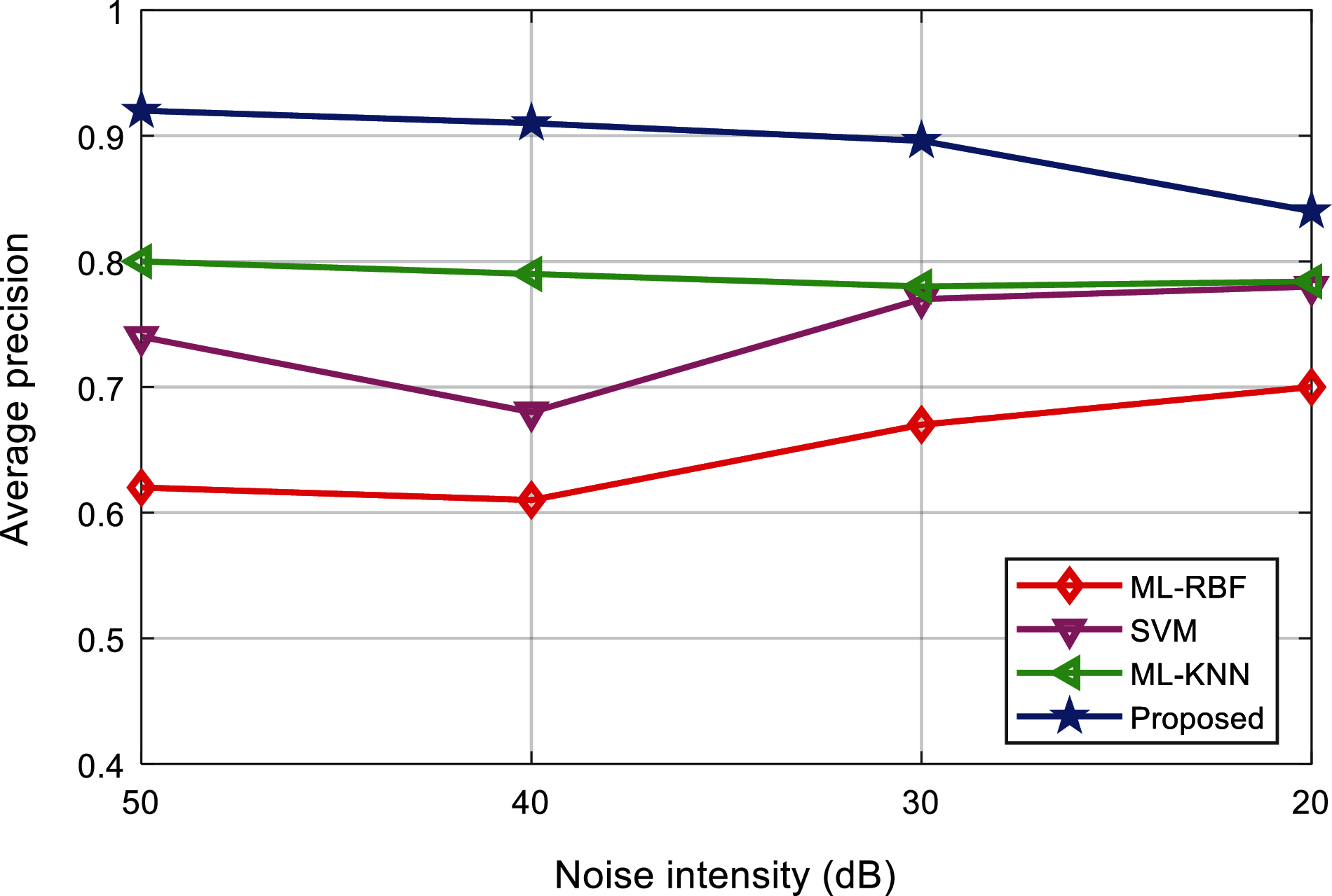
Figure 17: Comparison of the average precision of the algorithms
Tabs. 8 and 9 shows the training time and test time of the classification results of various interference signals under different noise levels. Figs. 18 and 19 shows the comparison results of the training time and test time of different classification methods. It can be found that, the proposed method can complete the training and testing within 10 s, and the classification efficiency advantage is obvious. It shows that, after the multi-label classification model based on the multi-layer extreme learning machine is trained, it can realize the rapid classification of power quality disturbances, which is suitable for the classification of a large number of interference signals.
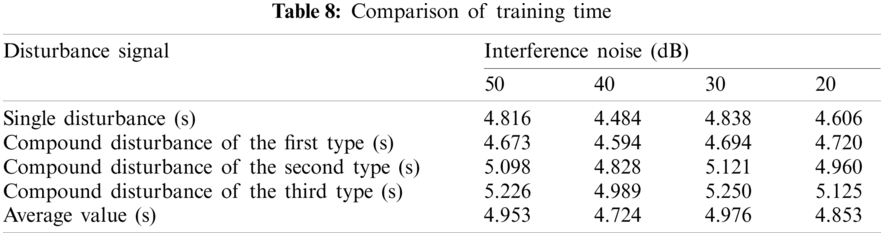
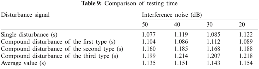
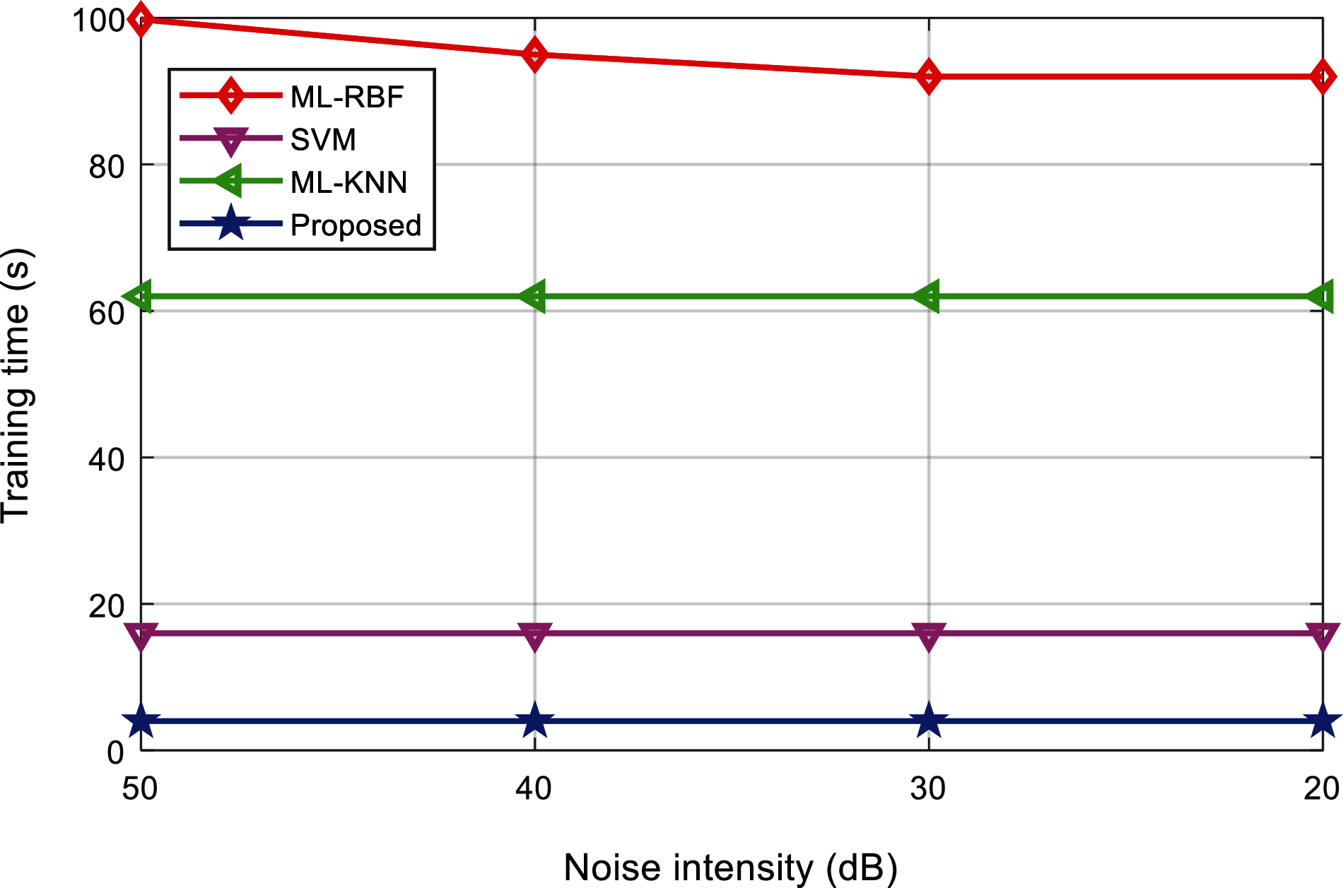
Figure 18: Comparison of training time of the algorithms
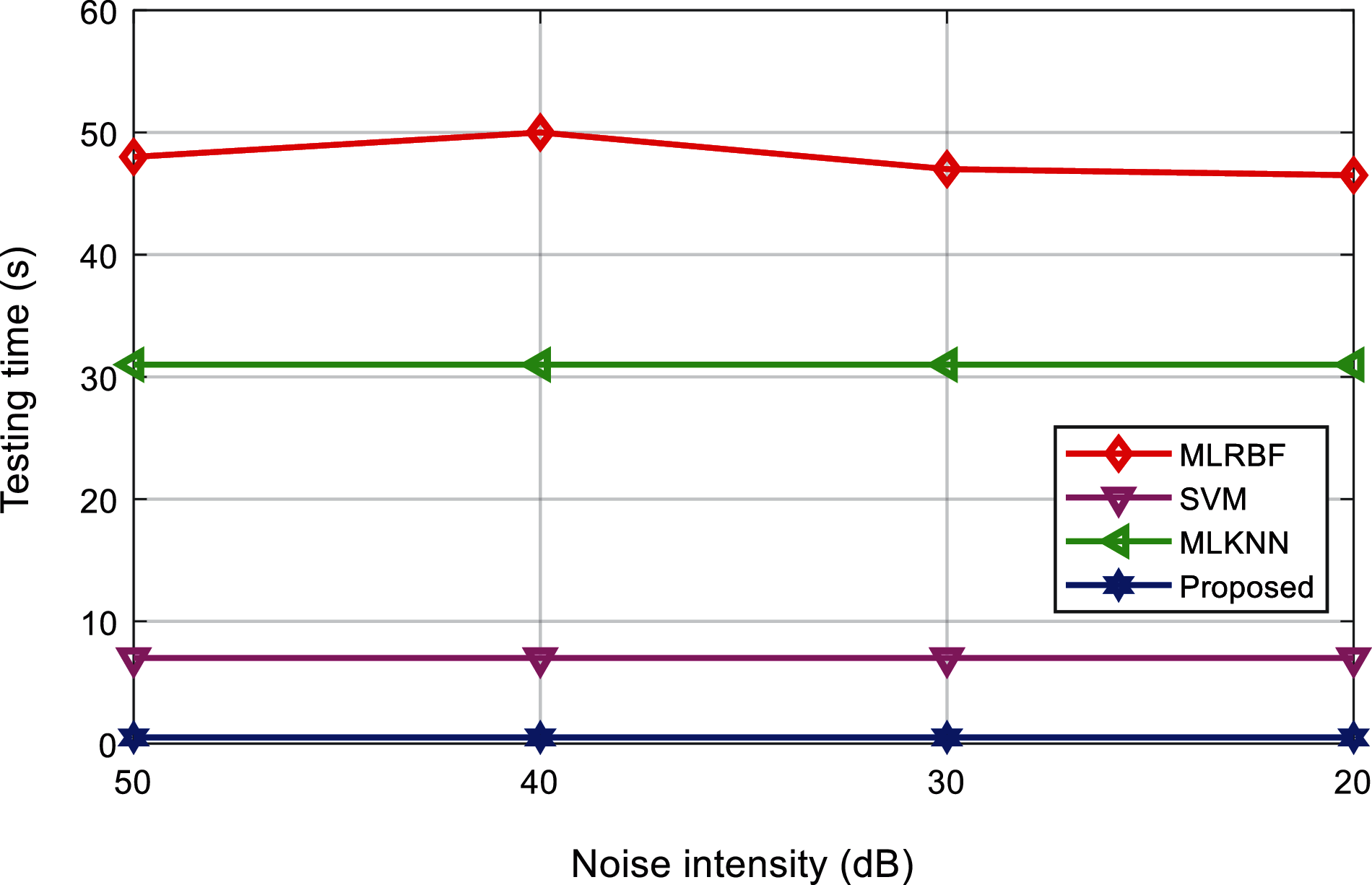
Figure 19: Comparison of testing time of the algorithms
Based on the above experimental results, the classifier model proposed in this paper has lower coverage rate, higher average accuracy, and Hamming loss, first-class error, ranking loss, and higher coverage than other classification methods. The proposed algorithm has a good classification effect and the training time and test time for classification are relatively low, showing higher classification efficiency.
First, the proposed algorithm includes the multiple hidden layers with strong nonlinear mapping capabilities and generalization capabilities, which can effectively characterize the complex interference signals and improve the average accuracy of classification.
Second, the proposed algorithm can extract a large amount of feature information, avoiding the contingency of random assignment of the algorithm. Under the interference of different intensities of noise, the variation of various performance indicators is small, and it has good generalization ability and robustness.
Third, the ranking-based multi-label classification algorithm fully considers the correlation between each label, and is suitable for the classification of single disturbance and compound disturbance, and has good anti-noise ability and classification accuracy.
Fourth, the proposed algorithm does not require iteration, reducing training time and testing time, and has obvious advantages when dealing with a large amount of power quality interference.
The power load of the grid in sTarbela is responsible for the power supply of 13 cities and regions and part of the power exchange between the three provinces of Punjab, Sindh and Balochistan. It has 11000 kV substation, 4500 kV substations, 28220 kV substations, and 110 kV substation 103. There are 18235 kV substations with a power supply capacity of 5.5 million kW. There are 621 35-220 kV lines with a line length of 8443.83 km.
This paper takes the electric energy disturbance as an example to study the application effect of the classification algorithm in the actual grid. According to the classification model and parameter range shown in the article, 100 training samples and 100 test samples are randomly selected for each type of power quality disturbance signal.
Tab. 10 shows the classification results of power quality disturbances and Fig. 20 shows the comparison of the classification results using different classification methods. Fig. 21 shows the comparison of the test time of different classification methods. It can be found that, the classification accuracy and testing of the proposed method in the actual power grid is basically the same as the simulation prediction results, and the classification effect and efficiency are significantly better than other methods.
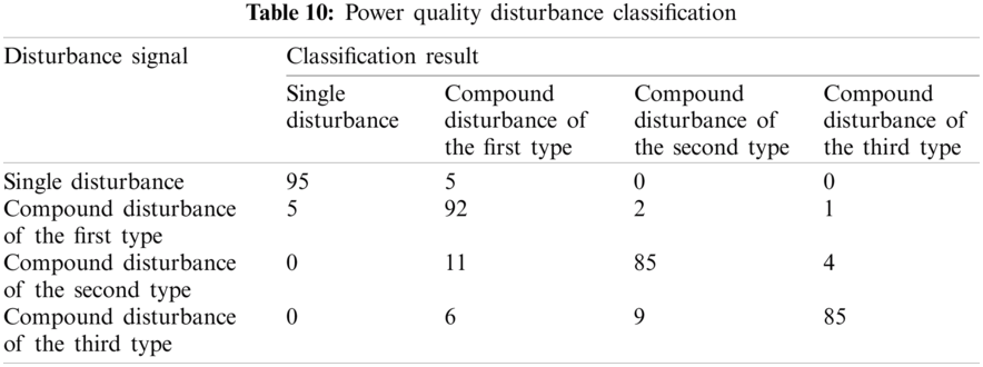
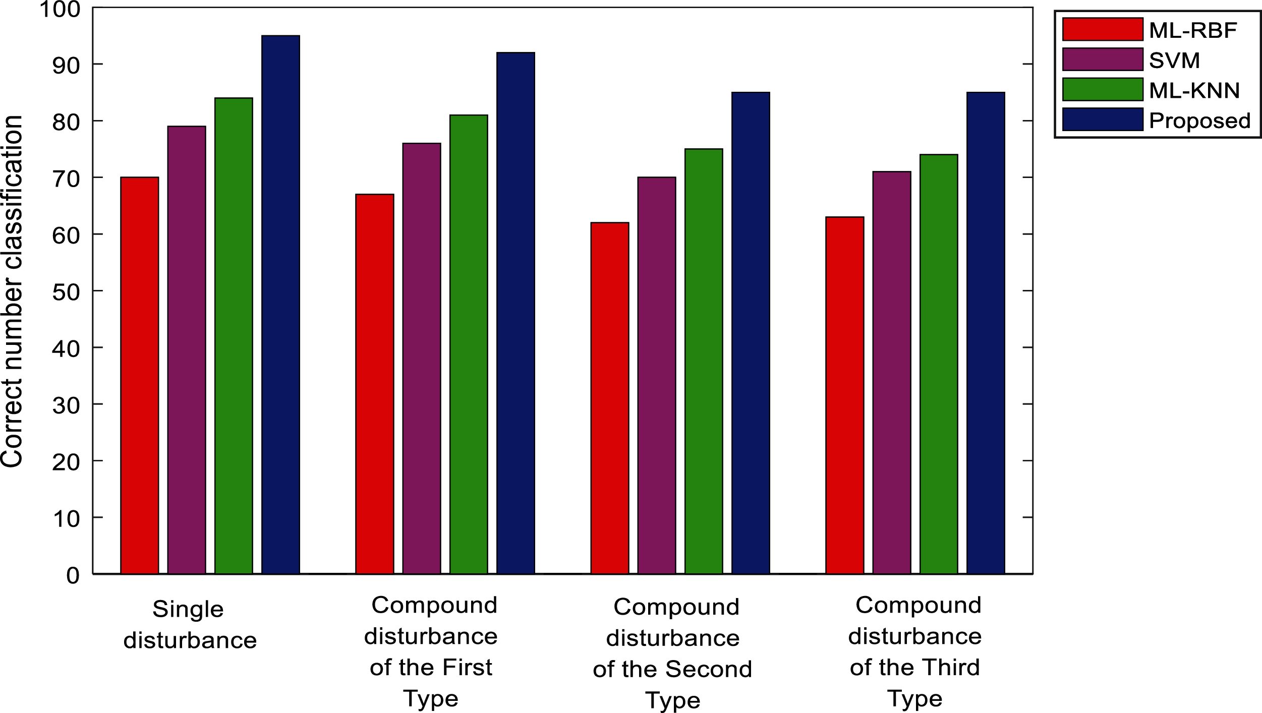
Figure 20: Power quality disturbance classification of the algorithms
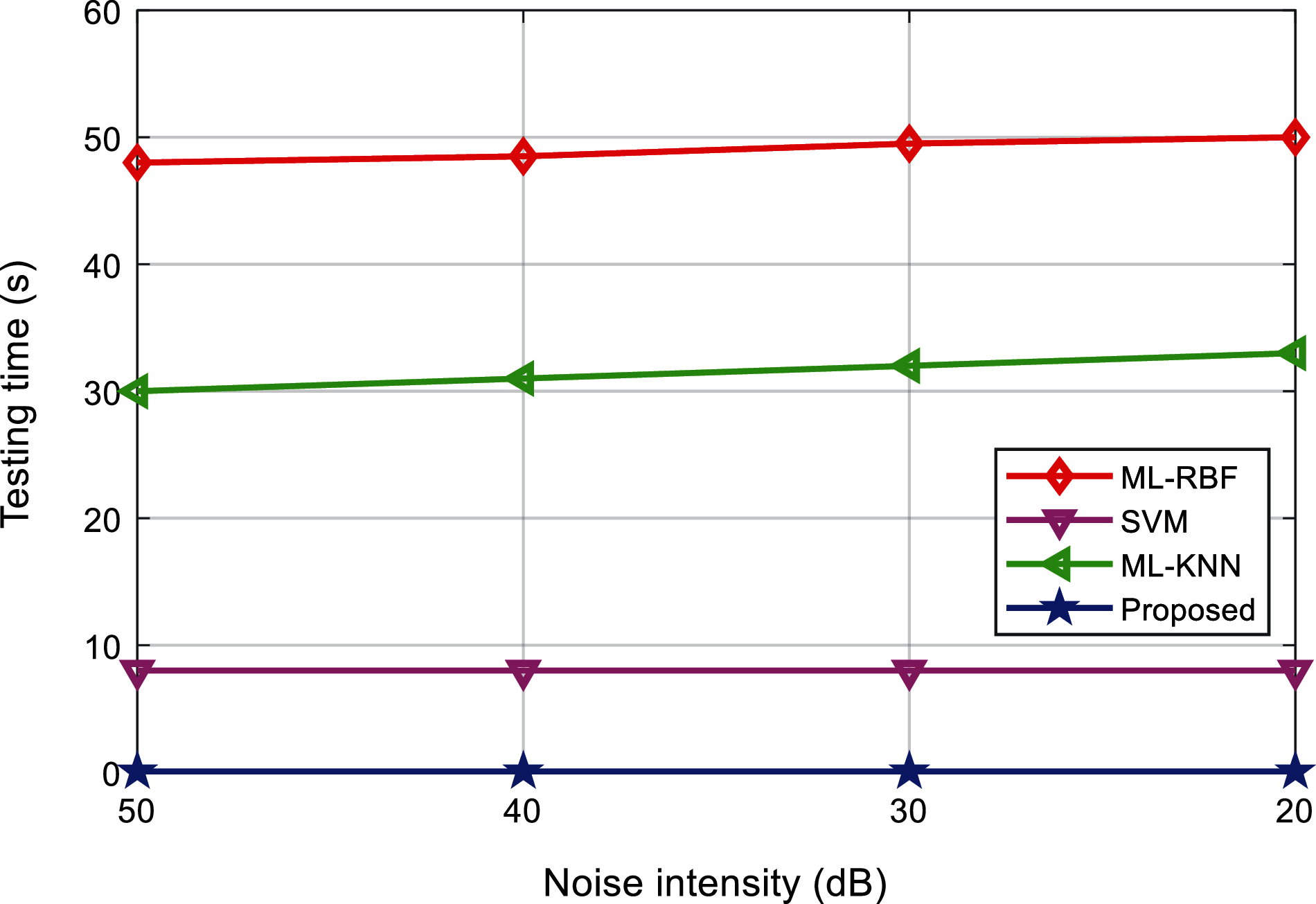
Figure 21: Testing time comparison of the algorithms
In this paper, combining the multi-layer extreme learning machine based on self-encoding and the multi-label classification algorithm based on ranking, a new power quality disturbance classification method is proposed, and the structure model and classification process of the classifier are explained. Experiments show that the proposed algorithm performs well in terms of Hamming loss, average accuracy, and coverage of the classification results, and has good noise resistance and robustness. It also significantly reduces the training time and test time, and the advantage is obvious when there are more interference signals. The proposed results provide effective means to determine the classification of disturbance in power signals quality. It can be generally deployed in relevant distribution networks that has to be evaluated in the context of disturbance analysis. Moreover, the proposed solution is optimal and has lower hamming loss, higher accuracy and improved ability to classify the disturbance. It has good anti-noise ability and high classification accuracy [50], and overcomes the randomness of traditional ELM parameter assignment, and has high classification efficiency, good robustness and generalization ability.
Funding Statement: The authors extend their appreciation to the Deanship of Scientific Research at Jouf University for funding this work through research Grant No. (DSR-2021-02-0203).
Conflicts of Interest: The authors declare that they have no conflicts of interest to report regarding the present study.
1. Q. Su, H. U. Khan, I. Khan, B. J. Choi, F. Wu et al., “An optimized algorithm for optimal power flow based on deep learning,” Energy Reports, vol. 7, pp. 2113–2124, 2021. [Google Scholar]
2. Z. Pan, N. V. Quynh, Z. M. Ali, S. Dadfar and T. Kashiwagi, “Enhancement of maximum power point tracking technique based on PV-battery system using hybrid bat algorithm and fuzzy controller,” Journal of Cleaner Production, vol. 274, no. 3, pp. 929–936, 2020. [Google Scholar]
3. M. H. Mostafa, S. E. Aleem, S. G. Ali, A. Y. Abdelaziz, P. Ribeiro et al., “Robust energy management and economic analysis of microgrids considering different battery characteristics,” IEEE Access, vol. 8, pp. 54751–54775, 2020. [Google Scholar]
4. N. V. Quynh, Z. M. Ali, M. M. Alhaider, A. Rezvani and K. Suzuki, “Optimal energy management strategy for a renewable-based microgrid considering sizing of battery energy storage with control policies,” International Journal of Energy Research, vol. 45, no. 4, pp. 5766–5780, 2021. [Google Scholar]
5. S. Khunkitti, A. Siritaratiwat, S. Premrudeepreechacharn, R. Chatthaworn and N. R. Watson, “A hybrid DA-PSO optimization algorithm for multiobjective optimal power flow problems,” Energies, vol. 11, no. 9, pp. 1–24, 2018. [Google Scholar]
6. Q. Alsafasfeh, O. A. Saraereh, I. Khan and S. Kim, “Solar PV grid power flow analysis,” Sustainability, vol. 11, no. 6, pp. 1–16, 2019. [Google Scholar]
7. Q. Alsafasfeh, O. A. Saraereh, I. Khan and S. Kim, “LS-Solar-pV system impact on line protection,” Electronics, vol. 8, no. 2, pp. 1–13, 2019. [Google Scholar]
8. Q. Alsafasfeh, O. A. Saraereh, I. Khan and B. J. Choi, “A robust decentralized power flow optimization for dynamic PV system,” IEEE Access, vol. 7, pp. 63789–63800, 2019. [Google Scholar]
9. Q. Alsafasfeh, O. A. Saraereh, M. Alsafasfeh, A. Maqableh, I. Khan et al., “An efficient algorithm for power flow optimization in PV inverters systems,” Electric Power Components and Systems, vol. 48, no. 12, pp. 1362–1377, 2020. [Google Scholar]
10. J. Radosavljevic, D. Klimenta, M. Jevtic and N. Arsic, “Optimal power flow using a hybrid optimization algorithm of particle swarm optimization and gravitational search algorithm,” Electric Power Components and Systems, vol. 43, no. 17, pp. 1958–1970, 2015. [Google Scholar]
11. M. Durairasan and D. Balasubramanian, “An efficient control strategy for optimal power flow management from a renewable energy source to a generalized three-phase microgrid systems: A hybrid squirrel search algorithm with whale optimization approach,” Transactions of the Institute of Measurement and Control, vol. 42, no. 11, pp. 321–331, 2020. [Google Scholar]
12. M. A. Shaheen, H. M. Hasanien and A. Al-Durra, “Solving of optimal power flow problem including renewable energy resources using HEAP optimization algorithm,” IEEE Access, vol. 9, pp. 35846–35863, 2021. [Google Scholar]
13. M. A. Shaheen, H. M. Hasanien, S. Mekhamer and H. E. Talaat, “Optimal power flow of power systems including distributed generations units using sunflower optimization algorithm,” IEEE Access, vol. 7, pp. 109289–109300, 2019. [Google Scholar]
14. M. Niu, C. Wan and Z. Xu, “A review on applications of heuristic optimization algorithms for optimal power flow in modern power systems,” Journal of Modern Power Systems and Clean Energy, vol. 2, no. 4, pp. 289–297, 2014. [Google Scholar]
15. H. T. Hassan, M. F. Tahir, K. Mehmood, K. M. Cheema, A. H. Milyani et al., “Optimization of power flow by Hamiltonian technique,” Energy Reports, vol. 6, pp. 2267–2275, 2020. [Google Scholar]
16. I. Kim, “The optimization of the location and capacity of reactive power generation units, using a hybrid genetic algorithm incorporated by the bus impedance power-flow calculation method,” Applied Sciences, vol. 10, no. 3, pp. 1–21, 2020. [Google Scholar]
17. M. A. Taher, S. Kamel, F. Jurado and M. Ebeed, “Optimal power flow solution incorporating a simplified UPFC model using lighting attachment procedure optimization,” International Transactions on Electrical Energy Systems, vol. 30, no. 1, pp. 1–22, 2020. [Google Scholar]
18. Y. Tang, K. Dvijotham and S. Low, “Real-time optimal power flow,” IEEE Transactions on Smart Grid, vol. 8, no. 6, pp. 2963–2973, 2017. [Google Scholar]
19. E. D. Anese and A. Simonetto, “Optimal power flow ursuit,” IEEE Transactions on Smart Grid, vol. 9, no. 2, pp. 942–952, 2016. [Google Scholar]
20. W. Warid, H. Hizam, N. Marium and N. I. A. Wahab, “Optimal power flow using the jaya algorithm,” Energies, vol. 9, no. 9, pp. 1–18, 2016. [Google Scholar]
21. L. Held, F. Mueller, S. Steinle, M. Barakat, M. R. Suriya et al., “An optimal power flow algorithm for the simulation of energy storage systems in unbalanced three-phase distribution grids,” Energies, vol. 14, no. 6, pp. 1–14, 2021. [Google Scholar]
22. A. Abdollahi, A. A. Ghadimi, M. R. Miveh, F. Mohammadi and F. Jurado, “Optimal power flow incorporating FACTS devices and stochastic wind power generation using kril herd algorithm,” Electronics, vol. 9, no. 6, pp. 1–17, 2020. [Google Scholar]
23. K. Nusair and L. Almoud, “Application of equilibrium optimizer algorithm for optimal power flow with high penetration of renewable energy,” Energies, vol. 13, no. 22, pp. 1–17, 2020. [Google Scholar]
24. B. V. Rao, F. Kupzog and M. Kozek, “Three-phase unbalanced optimal power flow using holomorphic embedding load flow method,” Sustainability, vol. 11, no. 3, pp. 1–16, 2019. [Google Scholar]
25. A. R. Baran and T. S. Fernandes, “A three-phase optimal power flow applied to the planning of unbalanced distribution networks,” International Journal of Electrical Power & Energy Systems, vol. 74, pp. 301–309, 2016. [Google Scholar]
26. Y. Chen, Z. Guo, H. Li, Y. Yang, A. Tadle et al., “Probabilistic optimal power flow for day-ahead dispatching of power systems with high-proportion renewable power sources,” Sustainability, vol. 12, no. 2, pp pp. 1–25, 2020. [Google Scholar]
27. H. Bouchekara, “Solution of the optimal power flow problem considering security constraints using an improved chaotic electromagnetic field optimization algorithm,” Neural Computing and Applications, vol. 32, pp. 2683–2703, 2020. [Google Scholar]
28. S. Duman, K. Li, L. Wu and U. Guvenc, “Optimal power flow with stochastic wind power and FACTS devices: A modified hybrid PSOGSA with chaotic maps approach,” Neural Computing and Applications, vol. 32, pp. 8463–8492, 2020. [Google Scholar]
29. S. S. Reddy, “Optimal power flow using hybrid differential evolution and harmony search algorithm,” International Journal of Machine Learning and Cybernetics, vol. 10, pp. 1077–1091, 2019. [Google Scholar]
30. M. Abbasi, E. Abbasi and B. M. Ivatloo, “Single and multi-objective optimal power flow using a new differential-based harmony search algorithm,” Journal of Ambient Intelligence and Humanized Computing, vol. 12, pp. 851–871, 2021. [Google Scholar]
31. M. Kaur and N. Narang, “An integrated optimization technique for optimal power flow solution,” Soft Computing, vol. 24, pp. 10865–10882, 2020. [Google Scholar]
32. J. Radosavljevic, M. Jevtic, N. Arsic and D. Klimenta, “Optimal power flow for distribution networks using gravitational search algorithm,” Electrical Engineering, vol. 96, pp. 335–345, 2014. [Google Scholar]
33. M. Zhang, “ML-Rbf: RBF neural networks for multi-label learning,” Neural Processing Letters, vol. 29, no. 2, pp. 61–74, 2009. [Google Scholar]
34. P. Chandrasekar and V. Kamraj, “Detection and classification of power quality disturbance waveform using mra based modified wavelet transform and neural networks,” Journal of Electrical Engineering, vol. 61, no. 4, pp. 235–240, 2010. [Google Scholar]
35. J. Huixian, “The analysis of plants image recognition based on deep learning and artificial neural network,” IEEE Access, vol. 8, pp. 68828–68841, 2020. [Google Scholar]
36. X. An, X. Zhou, X. Lu, F. Lin and L. Yang, “Sample selected extreme learning machine based intrusion detection in fog computing,” Wireless Communications and Mobile Computing, vol. 18, pp. 1–11, 2018. [Google Scholar]
37. M. Mishra, R. Panigrahi and P. K. Rout, “A combined mathematical morphology and extreme learning machine techniques based approach to micro-grid protection,” Ain Shams Engineering Journal, vol. 10, no. 2, pp. 307–318, 2019. [Google Scholar]
38. G. Li and J. Zou, “Multi-parallel extreme learning machine with excitatory and inhibitory neurons for regression,” Neural Processing Letters, vol. 51, pp. 1579–1597, 2020. [Google Scholar]
39. G. B. Huang, Q. Y. Zhu and C. K. Siew, “Extreme learning machine: Theory and applications,” Neurocomputing, vol. 70, no. 13, pp. 489–501, 2006. [Google Scholar]
40. W. Zhang, L. Shang and J. Sun, “Power quality disturbance classification based on time-frequency domain multifeature and decision tree,” Protection and Control of Modern Power Systems, vol. 4, no. 4, pp. 337–342, 2019. [Google Scholar]
41. A. Elisseeff and J. Weston, “A kernel method for multi-labelled classification,” in the 14th Int. Conf. on Neural Information Processing Systems, Vancouver, Canada, pp. 681–687, 2001. [Google Scholar]
42. U. Singh and S. N. Singh, “A new optimal feature selection scheme for classification of power quality disturbances based on any colony framework,” Applied Soft Computing, vol. 74, pp. 216–225, 2019. [Google Scholar]
43. J. C. Rodriguez, F. J. Torres and M. D. Borres, “Hybrid machine learning models for classifying power quality disturbances: A comparative study,” Energies, vol. 13, no. 11, pp. 1–20, 2020. [Google Scholar]
44. Z. Zheng, L. Qi, H. Wang, A. Pan and J. Zhou, “Recognition method of voltage sag causes based on two-dimensional transform and deep learning hybrid model,” IET Power Electronics, vol. 13, no. 1, pp. 168–177, 2020. [Google Scholar]
45. Q. L. Yang, J. M. Shao, M. Scholz, C. Boehm, C. Plant et al., “Multi-label classification models for sustainable flood retention basins,” Environmental Modelling & Software, vol. 32, pp. 27–36, 2012. [Google Scholar]
46. F. Guo, P. Wang, Y. Wang, P. Ren and Y. Zhang, “Research on improved s transform for the feature extraction of power quality,” IEEE Access, vol. 8, pp. 137910–137917, 2020. [Google Scholar]
47. J. Wang, Z. Xu and Y. Che, “Power quality disturbance classification based on compressed sensing and deep convolutional neural networks,” IEEE Access, vol. 7, pp. 78336–78346, 2019. [Google Scholar]
48. M. L. Zhang, P. Josem and R. Victor, “Feature selection for multi-label naïve Bayes classification,” Information Sciences, vol. 179, pp. 3218–3229, 2009. [Google Scholar]
49. S. K. Injeti and V. K. Thunuguntla, “Optimal integration of DGs into radial distribution network in the presence of plug-in electric vehicles to minimize daily active power losses and to improve the voltage profile of the system using bioinspired optimization algorithms,” Protection and Control of Modern Power Systems, vol. 5, no. 5, pp. 21–35, 2020. [Google Scholar]
50. S. Hasheminejad, E. Esmaeili and S. Jazebi, “Power quality disturbance classification using S-transform and hidden markov model,” Electric Power Components and Systems, vol. 40, no. 10, pp. 1160–1182, 2012. [Google Scholar]
51. M. R. Ravari, M. Eftekhari and F. S. Movahed, “Regularizing extreme learning machine by dual locally linear embedding manifold learning for training multi-label neural network classifiers,” Engineering Applications of Artificial Intelligence, vol. 97, pp. 1–23, 2021. [Google Scholar]
52. P. Vincent, H. Larochelle, Y. Bengio and P. A. Manzagol, “Extracting and composing robust features with denoising autoencoder,” in the 25th Int. Conf. on Machine Learning, Helsink, Finland, pp. 1096–1103, 2008. [Google Scholar]
53. D. A. Monteiro, W. G. Zvietcovich and M. F. Braga, “Detection and classification of power quality disturbances with wavelet transform, decision tree algorithm and support vector machine,”IEEE Simposio Brasileiro de Sistemas Eletricos (SBSENiteroi, Brazil, pp. 1–7, 2018. [Google Scholar]
54. M. Uyar, S. Yildirim and M. T. Gencoglu, “An effective wavelet-based feature extraction method for classification of power quality disturbance signals,” Electric Power Systems Research, vol. 78, no. 10, pp. 1747–1755, 2008. [Google Scholar]
55. A. M. Youssef, T. K. Abdelgalil, E. F. Elsaadany and M. Salama, “Disturbance classification utilizing dynamic time warping classifier,” IEEE Transactions on Power Delivery, vol. 19, no. 1, pp. 272–278, 2004. [Google Scholar]
56. N. M. Khoa and L. V. Dai, “Detection and classification of power quality disturbances in power system using modified-combination between the stockwell transform and decision tree methods,” Energies, vol. 13, no. 14, pp. 1–23, 2020. [Google Scholar]
57. M. Mohammadi, M. Afrasiabi, S. Afrasiabi and B. Parang, “Detection and classification of multiple power quality disturbances based on temporal deep learning,” in IEEE Int. Conf. on Environment and Electrical Engineering, Genova, Italy, pp. 1–6, 2019. [Google Scholar]
 | This work is licensed under a Creative Commons Attribution 4.0 International License, which permits unrestricted use, distribution, and reproduction in any medium, provided the original work is properly cited. |