[BACK]
Computers, Materials & Continua
DOI:10.32604/cmc.2022.022064 |  |
| Article | |
Metric-Based Resolvability of Quartz Structure
Muhammad Imran1,*, Ali Ahmad2, Muhammad Azeem3 and Kashif Elahi4
1Department of Mathematical Sciences, United Arab Emirates University, Al Ain, United Arab Emirates
2College of Computer Science & Information Technology Jazan University, Jazan, Saudi Arabia
3Department of Aerospace Engineering, Faculty of Engineering, Universiti Putra Malaysia, Malaysia
4Deanship of E-learning and Information Technology, Jazan University, Jazan, Saudi Arabia
*Corresponding Author: Muhammad Imran. Email: imrandhab@gmail.com
Received: 26 July 2021; Accepted: 22 September 2021
Abstract: Silica has three major varieties of crystalline. Quartz is the main and abundant ingredient in the crust of our earth. While other varieties are formed by the heating of quartz. Silica quartz is a rich chemical structure containing enormous properties. Any chemical network or structure can be transformed into a graph, where atoms become vertices and the bonds are converted to edges, between vertices. This makes a complex network easy to visualize to work on it. There are many concepts to work on chemical structures in terms of graph theory but the resolvability parameters of a graph are quite advance and applicable topic. Resolvability parameters of a graph is a way to getting a graph into unique form, like each vertex or edge has a unique identification by means of some selected vertices, which depends on the distance of vertices and its pattern in a particular graph. We have dealt some resolvability parameters of SiO2 quartz. We computed the resolving set for quartz structure and its variants, wherein we proved that all the variants of resolvability parameters of quartz structures are constant and do not depend on the order of the graph.
Keywords: Quartz; polycyclic aromatic hydrocarbon related structure;; metric dimension; metric or distance-based resolvability parameters
1 Introduction
Molecular graph is a simple graph transformed from a chemical network or a structure. While drawing it, the atom is represented as a vertex and the bond between two vertices is known as edge. This concept is usually chosen for the complex and huge network. Because the huge and complex network is toilsome to visualize but when it comes to a graph, it becomes easy to see the entire complex network into understandable format. This method is common in chemical graph theory or wherever huge network and complex structures exist. This way of looking into a structure is helpful because it makes the properties of the structure more comprehensible.
When each vertex or edge has unique identification, position or representation with respect to some other selected vertices, a huge molecular structure is shown off into a numerical representation. These mathematical representations are unique either for each vertex or edge or both. By this means, the physical properties of a chemical structure can be studied more deeply. A few vertices are selected with a condition that each vertex exhibits a unique identification, representation or location to the entire set of vertices in terms of distance or distance vector. This concept is named as locating set, resolving or metric basis by [1,2]. It has served multifariously especially in networking, robotizing and puzzle games. Later, its variety came up with different names and concepts, in which the next most attractive one is when a vertex is stopped working amongst the selected vertices. To overcome this situation, fault-tolerant concept is used. Actually, it is the extension of metric basis and named as fault-tolerant metric basis and developed by [3]. Now, instead of getting unique position of vertices, the requirement is to achieve the location of each edge uniquely in terms of selected vertices just as in metric basis. This idea also is the backbone in metric basis and is called edge metric basis and derived by [4]. In this concept the only change is getting the unique position of edges instead of vertices. The fault-tolerant case of edge parameter is introduced by [5], In which the failure of single vertex among the selected vertices is controllable or bearable. The graph theorist in [6] introduced the most complex parameter named as partition metric basis or partition resolving set. When the entire vertex set is rearranged into subsets and fulfilling the same condition of obtaining the unique position of each vertex. Formally, this group of parameters is called the resolvability parameters of a graph in a compact form.
The researchers in [6-9], discussed the complexity of all the definitions studied in this work. They proved that the computational cost of these concepts is NP-hardness problems or non-deterministic polynomial time problem. The very first parameter which is metric dimension, has enormous applications in different aspects. For example, in the seminal work of this definition by [1], the authors proposed the idea of using metric dimension in the coastguard Loran, facility location and sonar problems. Later, [10] associated this idea with the computer networks. Recognizing of image and for processing this idea is used by [11,12]. It can be applicable in coin weighing problems [13]. Image processing also leads this idea for robot navigation and discussed in [14]. The researcher in [15] linked this definition with the idea of combinatorial optimization and in usual manner which is always applicable when it comes to graph theory, this idea is also used in pharmaceutical chemistry [9].
Such as metric partition is also gaining a lot of interest due to its vast application in networking. Such as again in robot related study of this definition can be found in [14]. It is used for guiding and for the piloting of robot. A particular example of networking related to this idea, is available in [16]. The authors of [3] relate this idea with the famous Djokovic-Winkler relation. The puzzles also gain interest from this definition and discussion is available in [17]. Not all the applications are available here, one can search more data in [18-20].
The distance-based fault tolerant study of few basic graphs is available in [21], they discussed cycle path graphs and proved some bounds on general graphs related to this parameter. Mostly the fault-tolerant study associated with networks and useful in application point of view, [22] proved some results for this definition and also shows some applications in networking. Some chemical and computer structures are studied with this point of view and are available in [23-25]. A comparative discussion between vertex and edge version of metric dimension is available in [26]. For the edge version of metric parameter and studies have been intensively put forward in the last couple of years. A particular chemical structure is discussed in [27]. The general class of convex polytopes are discussed in the articles [28,29]. Another general class of graph obtained from different operations of graphs, is studied in [30]. General idea of metric which is known as partition dimension is discussed in [31-33], it provides a sharp utmost cardinality of partition metric basis. A particular type of fullerene was studied by [34]. Not always the cardinality of partition metric basis is constant but it can be in variation and changed by increasing the number of vertices, such a case is discussed in [35]. Now, the very first parameter of this case study, [36] develops a 3D hexagonal structure and provides the metric basis of this, they renamed it as locating number and provided some applications. A particular type of chemical structure is also studied by this parameter, for example α-boron nanotubes are discussed in [37], silicate star structure and its metric dimension are determined in [38] and cellulose network in [39]. Another structure of VC5C7 nanotubes is reshaped with this parameter and is available in [40]. The recent studies of all these parameters are available in [41].
The formal definitions of all the parameters studied or used in this work are elaborated below. Moreover, some basic relations are also given which are used to prove our main theorems.
Definition 1.1: Assume P be a simple undirected graph with the vertex set V(P) and E(P) edge set, the distance (geodesics) between α1,α2∈V(P) denoted by d(α1,α2), and calculated by counting the number of edges while moving through the α1−α2 path.
Definition 1.2: The main role in all the resolvability parameters is known as either location, position or representations and formally denoted by r(α|L) for the vertex α and L is the subset of selected vertices from the vertex set. Formally, let L={α1,α2,…,αi} is the subset of some selected vertices and α∈V(P). Now the vector (d(α,α1),d(α,α2),…,d(α,αi)) is a formal way of calculating the vector r(α|L). It is i-coordinate vector same as the cardinality of L. The necessary condition needs to put when choosing the subset of selected vertices, all the vertices from V(P) obtain a unique position, location or representation, in other words if all the coordinate of r(α|L) for each vertex is unique then L is a candidate for a resolving set. While the least number of members of L, is the metric dimension of graph P and it is formally shown by dim(P).
Definition 1.3: Let say there are i members in the resolving set for a graph, by eliminating all the members one by one from the set (α∈L,L∖α), if the condition of unique position (r(α|L)) holds for each vertex from the entire vertex set then L become (Lf) and known as fault-tolerant resolving set and similar way dimf(P) is the fault-tolerant metric dimension which is the minimum count of members of (Lf).
Definition 1.4: The distance between an edge e=α1α2∈E(P), and a vertex α∈V(P) is counted by the relation d(e,α)=min{d(α1,α),d(α2,α)}. Assuming a subset of selected vertices Le, if the position r(e|Le) of each e is unique of a graph then Le is called as edge metric resolving set and dime(p) is the minimum count of members of Le, called as edge metric dimension.
Definition 1.5: For the fault-tolerant edge metric resolving set we will follow the Definition 1.3. Let say there are i members in the edge metric resolving set for a graph, by eliminating all the members one by one from the set (α∈Le,Le∖α), if the condition of unique position (r(α|Le)) holds for each edge from the entire edge set then Le become (Le,f) and known as fault-tolerant edge metric resolving set and similar way dime,f(P) is the fault-tolerant edge metric dimension which is the minimum count of members of (Le,f).
Definition 1.6: The position vector r(α|Lp)={d(α,Lp1), d(α,Lp2),…, d(α,Lps)}, of a vertex α with respect to Lp. And the Lp is the s-ordered proper subset of vertex set and known as partition resolving set if position vector r(α|Lp) is unique for entire vertex set. The notation pd(P) is the minimum count of proper subsets of V(P) and called as partition dimension. It is the most complex parameter of metric-based resolvability parameters of a graph.
Now the following are few findings from literature and necessary for the concluding of our main results.
Theorem 1.7: [42] The inequality
dimf(P)≥dim(P)+1, is the sharp lower bound for the fault-tolerant metric dimension dimf(P) of a graph P, where dim(P) is the metric dimension of such graph P.
Theorem 1.8: [5] Similarly, the inequality
dime,f(P)≥dime(P)+1, is the sharp lower bound for the fault-tolerant edge metric dimension dime,f(P) of a graph P, where dime(P) is the edge metric dimension of such graph P.
Theorem 1.9: [1,43] The equation
dim(P)=dime(P)=1, holds only when P is a path graph, where dim(P) and dime(P) is the metric and edge metric dimension of such graph P, respectively.
2 Construction of SiO2 Quartz (Qk)
The graph shown in the Fig. 1 is the structure of polycyclic aromatic hydrocarbons from the benzenoid category of modern chemistry. It has 6k2+6k number of vertices and 9k2+3k number of edges. It has some particular families for the specific value of k. For example, benzene is the first member of polycyclic aromatic hydrocarbons family when k=1. The coronene and circumcoronene are the second and third family members of polycyclic aromatic hydrocarbons for the specific values of k=2,3 respectively. The resolvability parameters of this rich family of polycyclic aromatic hydrocarbons are studied in [41]. We will extend this work for the quartz structure shown in the Fig. 2 and is known as subdivision of polycyclic aromatic hydrocarbons.
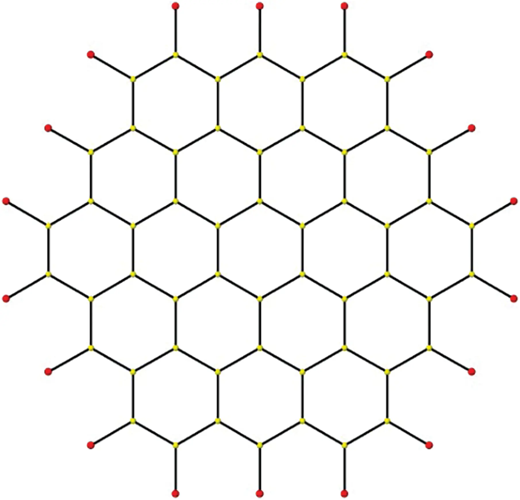
Figure 1: Polycyclic Aromatic Compound (PAHk)
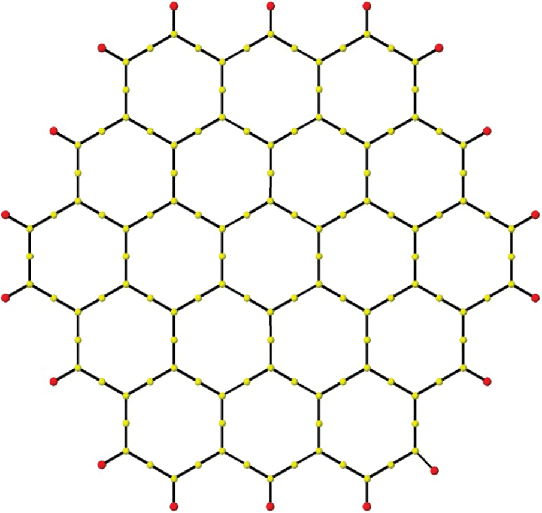
Figure 2: SiO2 Quartz (Qk)
Quartz is widely known by the structure of silicon dioxide and naturally occurring compound of silicon and oxygen. Quartz, cristobalite and tridymite are the three major crystalline varieties of silica. Among them, quartz is the most common polymorph of crystalline silica and can be found in huge amount in the earth's crust and is the single most abundant mineral that exists there. By treating the quartz at high temperature, cristobalite and tridymite are formed. The structure of quartz shown in Fig. 2 is the extension of polycyclic hydrocarbon structure shown in Fig. 1. Quartz is the subdivision of PAHk, each of the bond is subdivided into bonds by inserting two degree vertex. The clear and chemical view of Silica quartz is shown in the Fig. 2. Silica based nanomaterials and molecular belts have recently been found to be efficient in the drug delivery and transport due to their efficient resorption and desorption properties and their insolubility in water that helps in potential drug delivery system. Recently, many researchers throughout the world have contributed towards the study of chemical and physical properties of silicate structures such as tridymite and cristobalite [44-49]. It is noted that the pruned quartz with the removal of pendant bonds constitutes an interesting bridge for studies on silicon clusters [50,51] through laser vaporization techniques. In our study we focus on resolving the entire structure of silica quartz in terms of metric parameters. We found the exact metric, edge metric, fault-tolerant metric, fault-tolerant edge metric dimension and bounds of partition dimension of silica quartz which is denoted as Qk throughout the research work. Given below is the vertex set and edge set of associated graph of Qk.
V(Qk)={ai,j,bi,j:1≤i≤k,1≤j≤8k−4i+1}∪{ci,j,di,j:1≤i≤k−1,1≤j≤2k−i}∪{ei:1≤i≤2k}∪{fi,gi:1≤i≤3k}, E(Qk)={ai,jai,j+1,bi,jbi,j+1:1≤i≤k,1≤j≤8k−4i}∪{ai,jci,j′,bi,jdi,j′:1≤i≤k−1,3≤j≤8k−4i−1,j≡3(mod4),1≤j′≤2k−i}∪{ci,j′ai,j,di,j′bi,j:1≤i≤k−1,1≤j≤8k−4i−3,j≡1(mod4),1≤j′≤2k−i}∪{eia1,j,eib1,j:1≤i≤2k,1≤j≤8k−3,j≡1(mod4)}∪{ai,1fi,bi,1gi:1≤i≤k}∪{ak,jfi,bk,jgi:k+1≤i≤2k,3≤j≤4k−1,j≡3(mod4)}∪{ak−i+1,jfi′,bk−i+1,jgi′:1≤i≤k,2k+1≤i′≤3k,4k≤j≤8k−3,j≡1(mod4)}. The Fig. 3, shows the graph of Q3. In general, the quartz (Qk) has 15k2+3k total count of atoms or vertices and 18k2 are the bonds or edges. Moreover, from the V(Qk) and E(Qk) the generalize Qk can be produced. In our main results we will use the labeling of vertices defined in the Fig. 3 along with the help of vertex and edge set of Qk defined above.
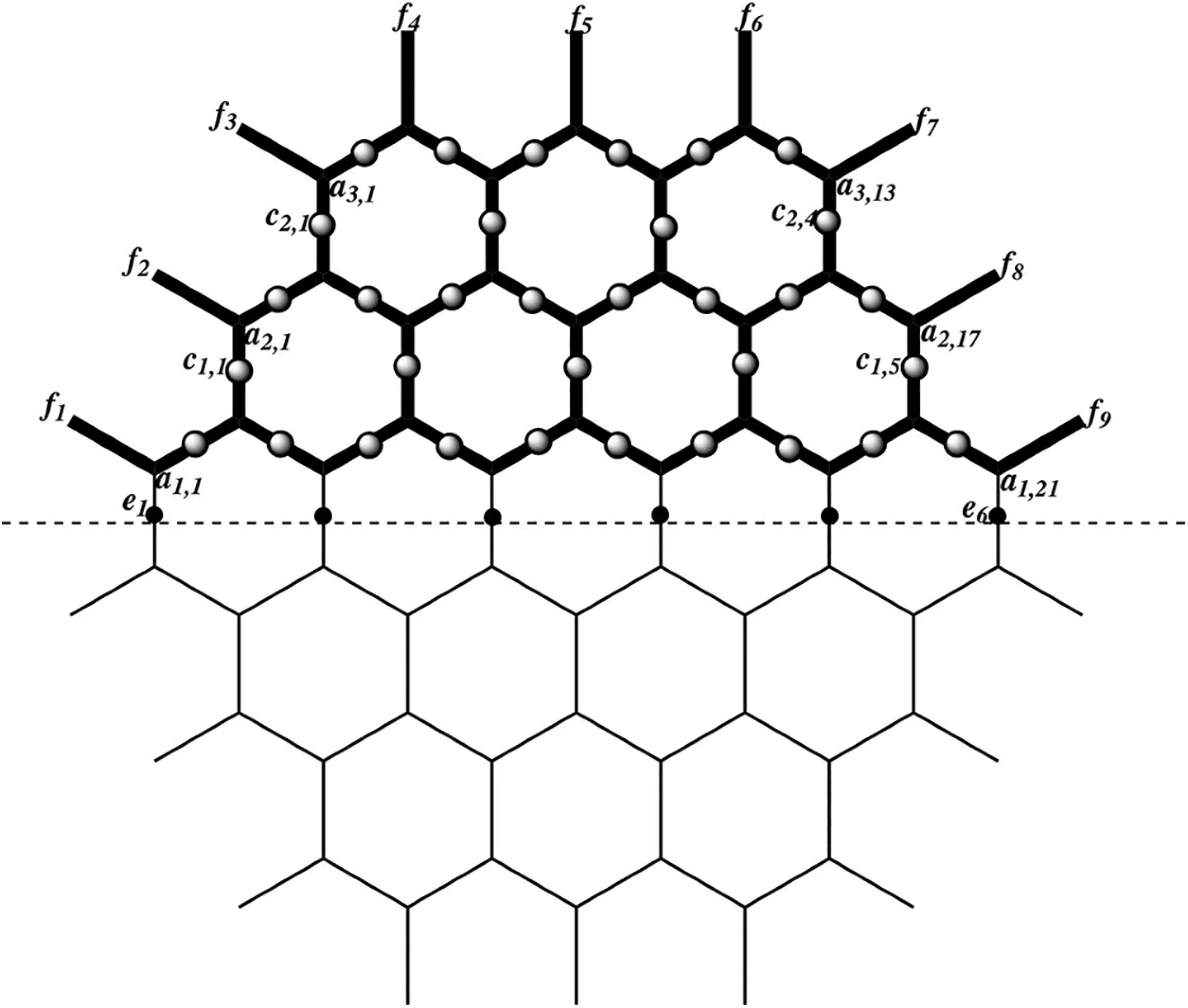
Figure 3: Quartz (Q3). The structure in the lower portion is similar to the upper one and atoms in the lower region of Q3 similarly can be labeled by bi,j,di,j, and gi.
3 Results on the Resolvability of SiO2 Quartz (Qk)
In this section we will reshape the structure of quartz (Qk) determining the different resolvability parameters. The very first lemma will play a role of landmark in the entire distance-based resolvability parameters. Later we will also discuss some other new and recent parameters in this section.
Lemma 3.1: Let Qk be a graph of quartz for k=1. Then the metric dimension of Qk is two.
Proof: To prove this Lemma, we will use the Definition 1.2 of metric dimension. As we claim that the structure of Q1 has metric dimension two, by the same definition we will assume a metric resolving set, say L={f1,f3}. Now the position or location vector for entire vertex of Q1 correspond to the subset L, is given in the Tab. 1.
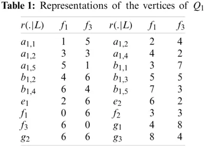
The location or positions for entire vertex set of Q1, given in the Tab. 1 are unique, which concludes the prove.
Lemma 3.2: Let Qk be a graph of quartz for k≥2. Then the resolving set of Qk has three cardinality.
Proof: To prove this lemma, we will use the Definition 1.2 of resolving set. As we claim that the structure of Qk has resolving set with three members, by the same definition we will assume a metric resolving set, say L={a1,1,b1,1,a1,8k−3}. Now the position or location vector for entire vertex of Qk correspond to the subset L, is given below.
For i=1,2,…,k, and j=1,2,…,8k−4i+1, The r(ai,j|L) and r(bi,j|L), are following;
r(ai,j|L)=(j+4i−5,j+4i−3,8k−j−3). r(bi,j|L)=(j+4i−3,j+4i−5,8k−j−1). For i=1,2,…,k−1, and j=1,2,…,2k−i, The r(ci,j|L) and r(di,j|L), are following;
r(ci,j|L)=(4j+4i−5,4j+4i−3,8k−4j−1). r(di,j|L)=(4j+4i−3,4j+4i−5,8k−4j+1). For i=1,2,…,k. The r(ei|L), are following;
r(ei|L)=(4i−3,4i−3,8k−4j+1). r(fi|L)={(4i−3,4i−1,8k−3),if i=1,2,…,k;(4i−5,4i−3,12k−4i−1),if i=k+1,k+2,…,2k;(8k−3,8k−1,12k−4i+1),if i=2k+1,2k+2,…,3k. r(gi|L)={(4i−1,4i−3,8k−1),if i=1,2,…,k;(4i−3,4i−5,12k−4i+1),if i=k+1,k+2,…,2k;(8k−1,8k−3,12k−4i+3),if i=2k+1,2k+2,…,3k. The location or positions for entire vertex set of Qk, given above are unique, which concludes the prove with the assertion that |L|=3.
Theorem 3.3: Let Qk be a graph of quartz for k≥2. Then
dim(Qk)=3. Proof: To prove this theorem, we will use the Definition 1.2 of metric dimension. As we claim that the structure of Qk has metric dimension three, by the same definition we will assume a metric resolving set, say L={a1,1,b1,1,a1,8k−3}. This subset of resolving set with certain selected vertices are already proved in Lemma 3.2. By choosing the double inequality method, we are left to prove that dim(Qk)≥3.
Now the assertion is dim(Qk)≥3, by contradiction let dim(Qk)=2. And let a resolving set L′ with |L′|=2. Given below are some cases to cover all possible combinations to make L′ with |L′|=2.
Case 1: Let L′⊂{ai,j:i=1, j=1,2,…,8k−4i+1}, with a condition that |L′|=2. Then the case resulted in same vertex's position and contradict our assumption with the fact that r(a2,j|L′)=r(b1,j|L′).
Case 2: Let L′⊂{ai,j:i=2,3,…,k−1 j=1,2,…,8k−4i+1}, with a condition that |L′|=2. Then the case resulted in same vertex's position and contradict our assumption with the fact that r(ai−1,j|L′)=r(ai+1,j|L′).
Case 3: Let L′⊂{ai,j:i=k,j=1,2,…,8k−4i+1}, with a condition that |L′|=2. Then the case resulted in same vertex's position and contradict our assumption with the fact that r(ak,j|L′)=r(a1,j|L′).
Case 4: Let L′⊂{bi,j:i=1,j=1,2,…,8k−4i+1}, with a condition that |L′|=2. Then the case resulted in same vertex's position and contradict our assumption with the fact that r(b2,j|L′)=r(a1,j|L′).
Case 5: Let L′⊂{bi,j:i=2,3,…,k−1 j=1,2,…,8k−4i+1}, with a condition that |L′|=2. Then the case resulted in same vertex's position and contradict our assumption with the fact that r(bi−1,j|L′)=r(bi+1,j|L′).
Case 6: Let L′⊂{bi,j:i=k,j=1,2,…,8k−4i+1}, with a condition that |L′|=2. Then the case resulted in same vertex's position and contradict our assumption with the fact that r(bk,j|L′)=r(b1,j|L′).
Case 7: Let L′⊂{fi:i=1,2,…,3k}, with a condition that |L′|=2. Then the case resulted in same vertex's position and contradict our assumption with the fact that r(a1,j|L′)=r(b1,j|L′).
Case 8: Let L′⊂{gi:i=1,2,…,3k}, with a condition that |L′|=2. Then the case resulted in same vertex's position and contradict our assumption with the fact that r(b1,j|L′)=r(a1,j|L′). By the fact that all the cases resulted in contradiction, then there does not exist a single possibility for L′, with |L′|=2, from the possible combinations which are |V|C2=|V|!2!(|V|−2)!=(15k2+3k)!2×(15k2+3k−2) of the entire vertex set of Qk. This indicate that the metric dimension of Qk two is not possible. Implied that dim(Qk)≥3.
Hence,
dim(Qk)=3. Lemma 3.4: Let Qk be a graph of quartz for k=1. Then the fault-tolerant metric dimension of Qk is three.
Proof: To prove this lemma, we will use the Definition 1.3 of fault-tolerant resolving set. As we claim that the structure of Q1 has fault-tolerant resolving set with three members, by the same definition we will assume a fault-tolerant metric resolving set, say Lf={f1,f3,g2}. Now the position or location vector for entire vertex of Q1 correspond to the subset Lf, is given in the Tab. 2.
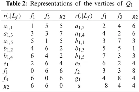
The location or positions for entire vertex set of Q1, given in the Tab. 2 are unique, which concludes the prove.
Lemma 3.5: Let Qk be a graph of quartz for k≥2. Then the cardinality of fault-tolerant resolving set of Qk is four.
Proof: To prove this lemma, we will use the Definition 1.3 of fault-tolerant resolving set. As we claim that the structure of Qk has fault-tolerant resolving set with four members, by the same definition we will assume a fault-tolerant metric resolving set, say Lf={a1,1,b1,1,a1,8k−3,b1,8k−3}. Now the position or location vector for entire vertex of Qk correspond to the subset Lf. is given below.
For i=1,2,…,k, and j=1,2,…,8k−4i+1, The r(ai,j|L) and r(bi,j|L), are following;
r(ai,j|Lf)=(j+4i−5,j+4i−3,8k−j−3,8k−j−1). r(bi,j|Lf)=(j+4i−3,j+4i−5,8k−j−1,8k−j−3). For i=1,2,…,k−1, and j=1,2,…,2k−i, The r(ci,j|L) and r(di,j|L), are following;
r(ci,j|Lf)=(4j+4i−5,4j+4i−3,8k−4j−1,8k−4j+1). r(di,j|Lf)=(4j+4i−3,4j+4i−5,8k−4j+1,8k−4j−1). For i=1,2,…,k. The r(ei|L), are following;
r(ei|Lf)=(4i−3,4i−3,8k−4j+1,8k−4j+1). r(fi|Lf)={(4i−3,4i−1,8k−3,8k−1),if i=1,2,…,k;(4i−5,4i−3,12k−4i−1,12k−4i+1),if i=k+1,k+2,…,2k;(8k−3,8k−1,12k−4i+1,12k−4i+3),if i=2k+1,2k+2,…,3k. r(gi|Lf)={(4i−1,4i−3,8k−1,8k−3),if i=1,2,…,k;(4i−3,4i−5,12k−4i+1,12k−4i−1),if i=k+1,k+2,…,2k;(8k−1,8k−3,12k−4i+3,12k−4i+1),if i=2k+1,2k+2,…,3k. The location or positions for entire vertex set of Qk, given above are unique, which concludes the prove with the assertion that |Lf|=4.
Theorem 3.6: Let Qk be a graph of quartz for k≥2. Then
dimf(Qk)=4. Proof: To prove this theorem, we will use the Definition 1.3 of fault-tolerant metric dimension. As we claim that the structure of Qk has fault-tolerant metric dimension four, by the same definition we will assume a fault-tolerant metric resolving set, say Lf={a1,1,b1,1,a1,8k−3,b1,8k−3}. This subset of fault-tolerant resolving set with certain selected vertices are already proved in Lemma 3.5. By choosing the double inequality method, we are left to proved that dimf(Qk)≥4.
Now the assertion dimf(Qk)≥4, and on contrary it become resulted in dimf(Qk)=3. Now by combining results from the Theorem 1.7 with Theorem 3.3. This completes the prove with the statement that dimf(Qk)≥4, and three fault-tolerant metric dimensions of Qk is not possible.
Hence
dimf(Qk)=4. Lemma 3.7: Let Qk be a graph of quartz for k=1. Then the edge metric dimension of Qk is two.
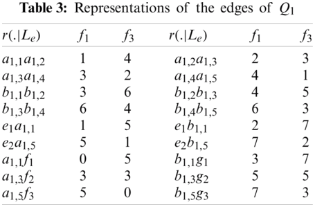
Proof: To prove this lemma, we will use the Definition 1.4 of edge resolving set. As we claim that the structure of Q1 has edge resolving set with two members, by the same definition we will assume an edge metric resolving set, say Le={f1,f3}. Now the position or location vector for entire edge set of Q1 correspond to the subset Le, is given in the Tab. 3.

The location or positions for entire edge set of Q1, given in the Tab. 3 are unique, which concludes the prove.
Lemma 3.8: Let Qk be a graph of quartz for k≥2. Then the edge metric resolving set of Qk has three cardinalities.
Proof: To prove this lemma, we will use the Definition 1.4 of edge resolving set. As we claim that the structure of Qk has edge resolving set with three members, by the same definition we will assume an edge metric resolving set, say Le={a1,1,b1,1,a1,8k−3}. Now the position or location vector for entire edge set of Qk correspond to the subset Le. is given below.
For i=1,2,…,k, and j=1,2,…,8k−4i, The r(ai,jai,j+1|Le) and r(bi,jbi,j+1|Le), are following;
r(ai,jai,j+1|Le)=(4i+j−5,4i+j−3,8k−j−4). r(bi,jbi,j+1|Le)=(4i+j−3,4i+j−5,8k−j−2). For i=1,2,…,k−1,j=3,7,11,…,8k−4i−1, and j′=1,2,…,2k−i, The r(ai,jci,j′|Le) and r(bi,jdi,j′|Le), are following;
r(ai,jci,j′|Le)=(4i+j−5,4i+j−3,8k−4i−2). r(bi,jdi,j′|Le)=(4i+j−3,4i+j−5,8k−4i). For i=1,2,…,k−1, j=1,5,9,…,8k−4i−3, and j′=1,2,…,2k−i, The r(ci,j′ai,j|Le) and r(di,j′bi,j|Le), are following;
r(ci,j′ai,j|Le)=(4i+j−2,4i+j,8k−4i−1). r(di,j′bi,j|Le)=(4i+j,4i+j−2,8k−4i+1). For i=1,2,…,2k, and j=1,5,9,…,8k−3, The r(eia1,j|Le) and r(eib1,j|Le), are following;
r(eia1,j|Le)=(4i−4,4i−3,8k−4i). r(eib1,j|Le)=(4i−3,4i−4,8k−4i+1). For i=1,2,…,k, The r(ai,1fi|Le) and r(bi,1gi|Le), are following;
r(ai,1fi|Le)=(4i−4,4i−2,8k−4). r(bi,1gi|Le)=(4i−2,4i−4,8k−2). For i=k+1,k+2,…,2k, and j=3,7,11,…,4k−1, The r(ak,jfi|Le) and r(bk,jgi|Le), are following;
r(ak,jfi|Le)=(4i−6,4i−4,12k−4i−2). r(bk,jgi|Le)=(4i−4,4i−6,12k−4i). For i=1,2,…,k,i′=2k+1,2k+2,…,3k, and j=4k+1,4k+5,4k+9,…,8k−3, The r(ak−i+1,jfi′|Le) and r(bk−i+1,jgi′|Le), are following;
r(ak−i+1,jfi′|Le)=(8k−4,8k−2,12k−4i). r(bk−i+1,jgi′|Le)=(8k−2,8k−4,12k−4i+2). The location or positions for entire edge set of Qk, given above are unique, which concludes the prove with the assertion that |Le|=3.
Theorem 3.9: Let Qk be a graph of quartz for k≥2. Then
dime(Qk)=3. Proof: To prove this theorem, we will use the Definition 1.4 of edge metric dimension. As we claim that the structure of Qk has edge metric dimension three, by the same definition we will assume an edge metric resolving set, say Le={a1,1,b1,1,a1,8k−3}. This subset of edge metric resolving set with certain selected vertices are already proved in Lemma 3.8. By choosing the double inequality method, we are left to proved that dime(Qk)≥3.
Now the assertion is dime(Qk)≥3, by contradiction let dime(Qk)=2, And let an edge resolving set Le′ with |Le′|=2. Given below are some cases to cover all possible combinations to make Le′ with |Le′|=2.
Case 1: Let Le′⊂{ai,j:i=1, j=1,2,…,8k−4i+1}, with a condition that |Le′|=2. Then the case resulted in same edge's position and contradict our assumption with the fact that r(a1,jei|Le′)=r(a1,ja2,j−1|Le′), where j=even, and i=1,2,…,2k.
Case 2: Let Le′⊂{ai,j:i=2,3,…,k−1, j=1,2,…,8k−4i+1}, with a condition that |Le′|=2. Then the case resulted in same edge's position and contradict our assumption with the fact that r(ai−1,jai−1,j′|Le′)=r(ai+1,jai+1,j′|Le′), where j′=1,2,…,8k−4i+1.
Case 3: Let Le′⊂{ai,j:i=k, j=1,2,…,8k−4i+1}, with a condition that |Le′|=2. Then the case resulted in same edge's position and contradict our assumption with the fact that r(ak,jak,j′|Le′)=r(a1,ja1,j′|Le′), where j′=1,2,…,8k−4i+1.
Case 4: Let Le′⊂{bi,j:i=1, j=1,2,…,8k−4i+1}, with a condition that |Le′|=2. Then the case resulted in same edge's position and contradict our assumption with the fact that r(a1,jb1,j|Le′)=r(b1,jb2,j−1|Le′), where j=even.
Case 5: Let Le′⊂{bi,j:i=2,3,…,k−1, j=1,2,…,8k−4i+1}, with a condition that |Le′|=2. Then the case resulted in same edge's position and contradict our assumption with the fact that r(bi−1,jbi−1,j′|Le′)=r(bi+1,jbi+1,j′|Le′), where j′=1,2,…,8k−4i+1.
Case 6: Let Le′⊂{bi,j:i=k, j=1,2,…,8k−4i+1}, with a condition that |Le′|=2. Then the case resulted in same edge's position and contradict our assumption with the fact that r(bk,jbk,j′|Le′)=r(b1,jb1,j′|Le′), where j′=1,2,…,8k−4i+1.
Case 7: Let Le′⊂{fi:i=1,2,…,3k}, with a condition that |Le′|=2. Then the case resulted in same edge's position and contradict our assumption with the fact that r(a1,ja1,j+1|Le′)=r(b1,jb1,j+1|Le′).
Case 8: Let Le′⊂{gi:i=1,2,…,3k}, with a condition that |Le′|=2. Then the case resulted in same edge's position and contradict our assumption with the fact that r(a1,ja1,j+1|Le′)=r(b1,jb1,j+1|Le′). By the fact that all the cases resulted in contradiction, then there does not exist a single possibility for Le′ with |Le′|=2, from the possible combinations which are |V|C2=|V|!2!(|V|−2)!=(15k2+3k)!2×(15k2+3k−2) of the entire vertex set of Qk. This indicate that edge metric dimension of Qk two is not possible. Hence; dime(Qk)≥3.
Now by from both relation of inequalities, concluded in
dime(Qk)=3. Lemma 3.10: Let Qk be a graph of quartz for k=1. Then the fault-tolerant edge metric dimension of Qk is three.
Proof: To prove this lemma, we will use the Definition 1.5 of fault-tolerant edge resolving set. As we claim that the structure of Q1 has fault-tolerant edge resolving set with three members, by the same definition we will assume a fault-tolerant edge metric resolving set, say Le,f={f1,f3,g2}. Now the position or location vector for entire edge set of Q1 correspond to the subset Le,f, is given in the Tab. 4.
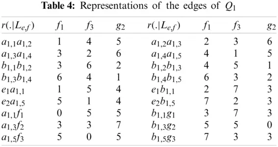
The location or positions for entire edge set of Q1, given in the Tab. 4 are unique, which concludes the prove.
Lemma 3.11: Let Qk be a graph of quartz for k≥2. Then the cardinality of fault-tolerant edge metric resolving set of Qk is four.
Proof: To prove this lemma, we will use the Definition 1.5 of fault-tolerant edge resolving set. As we claim that the structure of Qk has fault-tolerant edge resolving set with four members, by the same definition we will assume a fault-tolerant edge metric resolving set, say Le,f={a1,1,b1,1,a1,8k−3,b1,8k−3}. Now the position or location vector for entire edge set of Qk correspond to the subset Le,f. is given below.
For i=1,2,…,k, and j=1,2,…,8k−4i, The r(ai,jai,j+1|Le,f) and r(bi,jbi,j+1|Le,f), are following;
r(ai,jai,j+1|Le,f)=(4i+j−5,4i+j−3,8k−j−4,8k−j−2). r(bi,jbi,j+1|Le,f)=(4i+j−3,4i+j−5,8k−j−2,8k−j−4).
For i=1,2,…,k−1, j=3,7,11,…,8k−4i−1, and j′=1,2,…,2k−i, The r(ai,jci,j′|Le,f) and r(bi,jdi,j′|Le,f), are following;
r(ai,jci,j′|Le,f)=(4i+j−5,4i+j−3,8k−4i−2,8k−4i). r(bi,jdi,j′|Le,f)=(4i+j−3,4i+j−5,8k−4i,8k−4i−2). For i=1,2,…,k−1,j=1,5,9,…,8k−4i−3, and j′=1,2,…,2k−i, The r(ci,j′ai,j|Le,f) and r(di,j′bi,j|Le,f), are following;
r(ci,j′ai,j|Le,f)=(4i+j−2,4i+j,8k−4i−1,8k−4i+1). r(di,j′bi,j|Le,f)=(4i+j,4i+j−2,8k−4i+1,8k−4i−1). For i=1,2,…,2k, and j=1,5,9,…,8k−3, The r(eia1,j|Le,f) and r(eib1,j|Le,f), are following;
r(eia1,j|Le,f)=(4i−4,4i−3,8k−4i,8k−4i+1). r(eib1,j|Le,f)=(4i−3,4i−4,8k−4i+1,8k−4i). For i=1,2,…,k, The r(ai,1fi|Le,f) and r(bi,1gi|Le,f), are following;
r(ai,1fi|Le,f)=(4i−4,4i−2,8k−4,8k−2). r(bi,1gi|Le,f)=(4i−2,4i−4,8k−2,8k−4). For i=k+1,k+2,…,2k, and j=3,7,11,…,4k−1, The r(ak,jfi|Le,f) and r(bk,jgi|Le,f), are following;
r(ak,jfi|Le,f)=(4i−6,4i−4,12k−4i−2,12k−4i). r(bk,jgi|Le,f)=(4i−4,4i−6,12k−4i,12k−4i−2). For i=1,2,…,k,i′=2k+1,2k+2,…,3k, and j=4k+1,4k+5,4k+9,…,8k−3, The r(ak−i+1,jfi′|Le,f) and r(bk−i+1,jgi′|Le,f), are following;
r(ak−i+1,jfi′|Le,f)=(8k−4,8k−2,12k−4i,12k−4i+2). r(bk−i+1,jgi′|Le,f)=(8k−2,8k−4,12k−4i+2,12k−4i). The location or positions for entire edge set of Qk, given above are unique, which concludes the prove with the assertion that |Le,f|=4.
Theorem 3.12: Let Qk be a graph of quartz for k≥2. Then
dime,f(Qk)=4. Proof: To prove this theorem, we will use the Definition 1.5 of fault-tolerant edge metric dimension. As we claim that the structure of Qk has fault-tolerant edge metric dimension four, by the same definition we will assume a fault-tolerant edge metric resolving set, say Le,f={a1,1,b1,1,a1,8k−3,b1,8k−3}. This subset of fault-tolerant edge resolving set with certain selected vertices are already proved in Lemma 3.11. By choosing the double inequality method, we are left to proved that dime,f(Qk)≥4.
Now the assertion dime,f(Qk)≥4, and on contrary it become resulted in dime,f(Qk)=3, Now by combining results from the Theorem 1.8 with Theorem 3.9. This completes the prove with the statement that dime,f(Qk)≥4. and three fault-tolerant edge metric dimensions of Qk is not possible.
Hence
dime,f(Qk)=4. Lemma 3.13: Let Qk be a graph of quartz for k=1. Then the partition dimension of Qk is three.
Proof: To prove this lemma, we will use the Definition 1.6 of partition resolving set. As we claim that the structure of Q1 has partition resolving set with three members, by the same definition we will assume a partition resolving set, say Lp={Lp1,Lp2,Lp3,Lp4}, where Lp1={f1},Lp2={f3}, and Lp3=V(Qk)∖{f1,f3}. Now the position or location vector for entire vertex set of Q1 correspond to the subset Lp, is given in the Tab. 5.
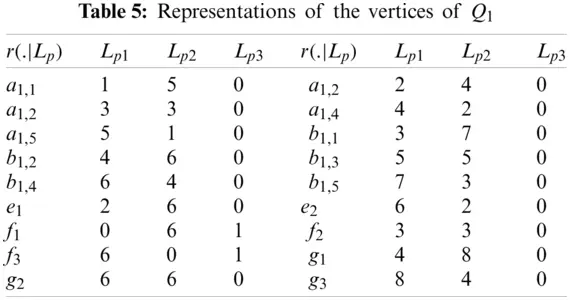
The location or positions for entire vertex set of Q1, given in the Tab. 5 are unique, which concludes the prove.
Lemma 3.14: Let Qk be the graphs of quartz for k≥2. Then the cardinality of partition resolving set of Qk is four.
Proof: To prove this lemma, we will use the Definition 1.6 of partition resolving set. As we claim that the structure of Qk has partition resolving set with four members, by the same definition we will assume a partition resolving set, say Lp={Lp1,Lp2,Lp3,Lp4}, where Lp1={a1,1},Lp2={b1,1},Lp3={a1,8k−3}, and Lp4=V(Qk)∖{a1,1,b1,1,a1,8k−3}. Now the position or location vector for entire vertex set of Qk correspond to the subset Lp, is given below.
For i=1,2,…,k, and j=1,2,…,8k−4i+1, The r(ai,j|L) and r(bi,j|L), are following;
r(ai,j|Lp)=(j+4i−5,j+4i−3,8k−j−3,z1). where z1={1,if i=j=1, andif i=1, j=8k−3;0,otherwise.
r(bi,j|Lp)=(j+4i−3,j+4i−5,8k−j−1,z2). where z2={1,if i=j=1;0,otherwise.
For i=1,2,…,k−1, and j=1,2,…,2k−i, The r(ci,j|Lp) and r(di,j|Lp), are following;
r(ci,j|Lp)=(4j+4i−5,4j+4i−3,8k−4j−1,0). r(di,j|Lp)=(4j+4i−3,4j+4i−5,8k−4j+1,0). For i=1,2,…,k. The r(ei|Lp), are following;
r(ei|Lp)=(4i−3,4i−3,8k−4j+1,0). r(fi|Lp)={(4i−3,4i−1,8k−3,0),if i=1,2,…,k;(4i−5,4i−3,12k−4i−1,0),if i=k+1,k+2,…,2k;(8k−3,8k−1,12k−4i+1,0),if i=2k+1,2k+2,…,3k. r(gi|Lp)={(4i−1,4i−3,8k−1,0),if i=1,2,…,k;(4i−3,4i−5,12k−4i+1,0),ifi=k+1,k+2,…,2k;(8k−1,8k−3,12k−4i+3,0),if i=2k+1,2k+2,…,3k. The location or positions for entire vertex set of Qk, given above are unique, which concludes the prove with the assertion that |Lp|=4.
Theorem 3.15: Let Qk be the graphs of quartz for k≥2. Then
pd(Qk)≤4. Proof: To prove this theorem, we will use the Definition 1.6 of partition dimension. As we claim that the structure of Qk has partition dimension less than or equal to four, by the same definition we will assume a partition resolving set, say Lp={Lp1,Lp2,Lp3,Lp4}, where Lp1={a1,1},Lp2={b1,1},Lp3={a1,8k−3}, and Lp4=V(Qk)∖{a1,1,b1,1,a1,8k−3}. This subset of partition resolving set with proper subsets of entire vertex are already proved in Lemma 3.14. As we can see in Lemma 3.14 the partition resolving set has the cardinality four. It is concluded that
pd(Qk)≤4. 4 Conclusion
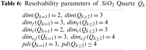
In this diverse study we have discussed SiO2 quartz Qk structure with different distance-based resolvability parameters. We concluded that all the parameters studied in this work are constant and do not depend on the variation of moving parameter k, despite when k=1 or k≥2. For all the rest values of k≥2, all the parameters remain unchanged and we provide general resolving set for vertex and edge version, fault-tolerant resolving set for vertex and edge version and at the end we concluded by taking the entire vertex set into four cardinality proper subsets. Moreover, the cardinality of all the parameters studied here are concluded in the following Tab. 6.

Funding Statement: This research is supported by the University program of Advanced Research (UPAR) and UAEU-AUA grants of United Arab Emirates University (UAEU) via Grant No. G00003271 and Grant No. G00003461.
Conflicts of Interest: The authors declare that they have no conflicts of interest to report regarding the present study.
References
1. F. Harary and R. A. Melter, “On the metric dimension of a graph,” Ars Combinatoria, vol. 2, pp. 191–195, 1976. [Google Scholar]
2. P. J. Slater, “Leaves of trees,” Proc. of the 6th Southeastern Conf. on Combinatorics, Graph Theory, and Computing, Congressus Numerantium, Florida Atlantic University, Boca Raton, vol. 14, pp. 549–559, 1975. [Google Scholar]
3. J. Caceres, C. Hernando, M. Mora, I. M. Pelayo, M. L. Puertas et al., “On the metric dimension of cartesian product of graphs,” SIAM Journal on Discrete Mathematics, vol. 2, pp. 423–441, 2007. [Google Scholar]
4. A. Kelenc, N. Tratnik and I. G. Yero, “Uniquely identifying the edges of a graph: The edge metric dimension,” Discrete Applied Mathematics, vol. 251, pp. 204–220, 2018. [Google Scholar]
5. X. Liu, M. Ahsan, Z. Zahid and S. Ren, “Fault-tolerant edge metric dimension of certain families of graphs,” AIMS Mathematics, vol. 6, no. 2, pp. 1140–1152, 2021. [Google Scholar]
6. G. Chartrand, E. Salehi and P. Zhang, “The partition dimension of graph,” Aequationes Mathematicae, vol. 59, pp. 45–54, 2000. [Google Scholar]
7. M. Hauptmann, R. Schmied and C. Viehmann, “Approximation complexity of metric dimension problem,” Journal of Discrete Algorithms, vol. 14, pp. 214–222, 2012. [Google Scholar]
8. H. R. Lewis, M. R. Garey and D. S. Johnson, “Computers and intractability. a guide to the theory of np-completeness,” Journal of Symbolic Logic, vol. 48, no no. 2, pp. 498–500, 1983. [Google Scholar]
9. Z. Beerliova, F. Eberhard, T. Erlebach, A. Hall, M. Hoffmann et al., “Network discovery and verification,” IEEE Journal on Selected Areas in Communications, vol. 24, no. 12, pp. 2168–2181, 2006. [Google Scholar]
10. P. Manuel, R. Bharati, I. Rajasingh and M. C. Monica, “On minimum metric dimension of honeycomb networks,” Journal of Discrete Algorithms, vol. 6, no. 1, pp. 20–27, 2008. [Google Scholar]
11. M. Perc, J. Gómez-Gardenes, A. Szolnoki, L. M. Floría and Y. Moreno “Evolutionary dynamics of group interactions on structured populations: A review,” Journal of the Royal Society Interface, vol. 10, no. 80, Article ID 20120997, 2013. https://doi.org/10.1098/rsif.2012.0997. [Google Scholar]
12. M. Perc and A. Szolnoki, “Coevolutionary games-a mini review,” Biosystems, vol. 99, no. 2, pp. 109–125, 2010. [Google Scholar]
13. S. Söderberg and H. S. Shapiro, “A combinatory detection problem,” The American Mathematical Monthly, vol. 70, no. 10, pp. 1066–1070, 1963. [Google Scholar]
14. S. Khuller, B. Raghavachari and A. Rosenfeld, “Landmarks in graphs,” Discrete Applied Mathematics, vol. 70, no. 3, pp. 217–229, 1996. [Google Scholar]
15. A. Sebö and E. Tannier, “On metric generators of graphs,” Mathematics and Operational Research, vol. 29, pp. 383–393, 2004. [Google Scholar]
16. G. Chartrand, L. Eroh, M. A. O. Johnson and R. Ortrud, “Resolvability in graphs and the metric dimension of a graph,” Discrete Applied Mathematics, vol. 105, pp. 99–113, 2000. [Google Scholar]
17. V. Chvatal, “Mastermind,” Combinatorica, vol. 3, pp. 325–329, 1983. [Google Scholar]
18. M. A. Johnson, “Structure-activity maps for visualizing the graph variables arising in drug design,” Journal of Biopharmaceutical Statistics, vol. 3, pp. 203–236, 1993. [Google Scholar]
19. S. Imran, M. K. Siddiqui and M. Hussain, “Computing the upper bounds for the metric dimension of cellulose network,” Applied Mathematics E-Notes, vol. 19, pp. 585–605, 2019. [Google Scholar]
20. R. A. Melter and I. Tomescu, “Metric bases in digital geometry,” Computer Vision Graphics and Image Processing, vol. 25, pp. 113–121, 1984. [Google Scholar]
21. M. Javaid, M. U. Rehman and J. Cao, “Topological indices of rhombus type silicate and oxide networks,” Canadian Journal of Chemistry, vol. 95, no. 2, pp. 134–143, 2016. [Google Scholar]
22. H. Raza, S. Hayat and X. F. Pan, “On the fault-tolerant metric dimension of certain interconnection networks,” Journal of Applied Mathematics and Computing, vol. 60, pp. 517–535, 2019. [Google Scholar]
23. H. Raza, S. Hayat, M. Imran and X. F. Pan, “Fault-tolerant resolvability and extremal structures of graphs,” Mathematics, vol. 7, pp. 78–97, 2019. [Google Scholar]
24. M. Somasundari and F. S. Raj, “Fault-tolerant resolvability of oxide interconnections,” International Journal of Innovative Technology and Exploring Engineering, vol. 8, pp. 2278–3075, 2019. [Google Scholar]
25. H. Raza, S. Hayat and X. F. Pan, “On the fault-tolerant metric dimension of convex polytopes,” Applied Mathematics and Computing, vol. 339, pp. 172–185, 2018. [Google Scholar]
26. Z. Raza and M. S. Bataineh, “The comparative analysis of metric and edge metric dimension of some subdivisions of the wheel graph,” Asian-European Journal of Mathematics, vol. 14, no. 4, article ID: 2150062, 2021. https://www.worldscientific.com/doi/10.1142/S1793557121500625. [Google Scholar]
27. A. N. A. Koam, A. Ahmad, M. Ibrahim and M. Azeem, “Edge metric and fault-tolerant edge metric dimension of hollow coronoid,” Mathematics, vol. 9, no. 12, article no. 1405, 2021. https://www.mdpi.com/2227-7390/9/12/1405. [Google Scholar]
28. Y. Zhang and S. Gao, “On the edge metric dimension of convex polytopes and its related graphs,” Journal of Combinatorial Optimization, vol. 39, no. 2, pp. 334–350, 2020. [Google Scholar]
29. M. Ahsan, Z. Zahid, S. Zafar, A. Rafiq, M. S. Sindhu et al., “Computing the edge metric dimension of convex polytopes related graphs,” Journal of Mathematics and Computer Science, vol. 22, no. 2, pp. 174–188, 2020. [Google Scholar]
30. A. N. A. Koam and A. Ahmad, “Barycentric subdivision of cayley graphs with constant edge metric dimension,” IEEE Access, vol. 8, pp. 80624–80628, 2020. [Google Scholar]
31. Y. M. Chu, M. F. Nadeem, M. Azeem and M. K. Siddiqui, “On sharp bounds on partition dimension of convex polytopes,” IEEE Access, vol. 8, pp. 224781–224790, 2020. [Google Scholar]
32. J. B. Liu, M. F. Nadeem and M. Azeem, “Bounds on the partition dimension of convex polytopes,” Combinatorial Chemistry and Throughput Screening, 2020. https://doi.org/10.2174/1386207323666201204144422. [Google Scholar]
33. A. Shabbir and M. Azeem, “On the partition dimension of tri-hexagonal alpha-boron nanotube,” IEEE Access, vol. 9, pp. 55644–55653, 2021. [Google Scholar]
34. M. F. Nadeem, M. Azeem and A. Khalil, “The locating number of hexagonal möbius ladder network,” Journal of Applied Mathematics and Computing, vol. 66, pp. 149–165, 2021. [Google Scholar]
35. E. T. Baskoro and D. O. Haryeni. “All graphs of order n≥11 and diameter 2 with partition dimension n−3,” Heliyon, vol. 6, no. 4, 2021, pp. e03694. https://doi.org/10.1016/j.heliyon.2020.e03694. [Google Scholar]
36. N. Mehreen, R. Farooq and S. Akhter, “On partition dimension of fullerene graphs,” AIMS Mathematics, vol. 3, no. 3, pp. 343–352, 2018. [Google Scholar]
37. Z. Hussain, M. Munir, M. Choudhary and S. M. Kang, “Computing metric dimension and metric basis of 2d lattice of alpha-boron nanotubes,” Symmetry, vol. 10, no. 8, article no. 300, 2018. https://www.mdpi.com/2073-8994/10/8/300. [Google Scholar]
38. F. Simonraj and A. George, “On the metric dimension of silicate stars,” ARPN Journal of Engineering and Applied Sciences, vol. 10, no. 5, pp. 2187–2192, 2015. [Google Scholar]
39. M. K. Siddiqui and M. Imran, “Computing the metric and partition dimension of h-naphtalenic and vc5c7 nanotubes,” Journal of Optoelectronics and Advanced Materials, vol. 17, pp. 790–794, 2015. [Google Scholar]
40. M. A. Johnson, “B rowsable Structure-Activity Datasets, Advances in Molecular Similarity,” Netherlands: JAI Press Connecticut, vol. 2, pp. 153–170, 1998. https://linkinghub.elsevier.com/retrieve/pii/S187397769880014X. [Google Scholar]
41. M. Azeem and M. F. Nadeem, “Metric-based resolvability of polycyclic aromatic hydrocarbons,” European Physical Journal Plus, vol. 136, article no. 395, 2021. https://doi.org/10.1140/epjp/s13360-021-01399-8. [Google Scholar]
42. M. A. Chaudhry, I. Javaid and M. Salman, “Fault-tolerant metric and partition dimension of graphs,” Utliltas Mathematica, vol. 83, pp. 187–199, 2010. [Google Scholar]
43. I. G. Yero. “Vertices, edges, distances and metric dimension in graphs,” Electronic Notes in Discrete Mathematics, vol. 55, pp. 191–194, 2016. [Google Scholar]
44. M. Arockiaraj, S. R. J. Kavitha and K. Balasubramanian, “Vertex cut method for degree and distance-based topological indices and its applications to silicate networks,” Journal of Mathematical Chemistry, vol. 54, no. 8, pp. 1728–1747, 2016. [Google Scholar]
45. M. Arockiaraj, S. R. J. Kavitha, K. Balasubramanian and I. Gutman, “Hyper-wiener and wiener polarity indices of silicate and oxide frameworks,” Journal of Mathematical Chemistry, vol. 55, no. 5, pp. 1493–1510, 2018. [Google Scholar]
46. M. Arockiaraj, S. Klavžar, S. Mushtaq and K. Balasubramanian, “Distance-based topological indices of sio2 nanosheets, nanotubes and nanotori,” Journal of Mathematical Chemistry, vol. 57, pp. 343–369, 2020. [Google Scholar]
47. A. Q. Baig, M. Imran and H. Ali, “On topological indices of poly oxide, poly silicate, dox, and dsl networks,” Canadian Journal of Chemistry, vol. 93, no. 7, pp. 730–739, 2015. [Google Scholar]
48. M. Javaid and C. Y. Jung, “M-polynomials and topological indices of silicate and oxide networks,” International Journal of Pure and Applied Mathematics, vol. 115, no. 1, pp. 129–152, 2017. [Google Scholar]
49. I. Javaid, M. Salman, M. A. Chaudhry and S. Shokat, “Fault-tolerance in resolvability,” Utliltas Mathematica, vol. 80, pp. 263–275, 2009. [Google Scholar]
50. K. Balasubramanian, “Cas scf/ci calculations on si4 and si4+,” Chemical Physics Letter, vol. 135, no. 3, pp. 283–287, 1987. [Google Scholar]
51. C. Zhao and K. Balasubramanian, “Geometries and spectroscopic properties of silicon clusters,” Journal of Chemistry and Physics, vol. 116, no. 9, pp. 3690–3699, 2002. [Google Scholar]