DOI:10.32604/cmc.2022.022451
| Computers, Materials & Continua DOI:10.32604/cmc.2022.022451 | |
| Article |
Takagi–Sugeno Fuzzy Modeling and Control for Effective Robotic Manipulator Motion
1Department of Automated Manufacturing, University of Baghdad, Baghdad, 10001, Iraq
2Department of Mechanical Engineering, University of Kirkuk, Kirkuk, 36001, Iraq
3Department of Computer Technical Engineering, Al-kitab University, Kirkuk, 36001, Iraq
4Higher Colleges of Technology, Abu Dhabi Women’s College, Abu Dhabi, 41012, UAE
5Department of Computer Science, University of Swat, Shangla Campus, Alpurai, 19100, Shangla, Pakistan
6Department of Mechatronics Engineering, Manipal University Jaipur, Jaipur, 302004, India
7Department of Computer Science & IT, University of Engineering & Technology Peshawar, Peshawar, 25000, Pakistan
*Corresponding Author: Sadeeq Jan. Email: sadeeqjan@uetpeshawar.edu.pk
Received: 06 August 2021; Accepted: 07 September 2021
Abstract: Robotic manipulators are widely used in applications that require fast and precise motion. Such devices, however, are prompt to nonlinear control issues due to the flexibility in joints and the friction in the motors within the dynamics of their rigid part. To address these issues, the Linear Matrix Inequalities (LMIs) and Parallel Distributed Compensation (PDC) approaches are implemented in the Takagy–Sugeno Fuzzy Model (T-SFM). We propose the following methodology; initially, the state space equations of the nonlinear manipulator model are derived. Next, a Takagy–Sugeno Fuzzy Model (T-SFM) technique is used for linearizing the state space equations of the nonlinear manipulator. The T-SFM controller is developed using the Parallel Distributed Compensation (PDC) method. The prime concept of the designed controller is to compensate for all the fuzzy rules. Furthermore, the Linear Matrix Inequalities (LMIs) are applied to generate adequate cases to ensure stability and control. Convex programming methods are applied to solve the developed LMIs problems. Simulations developed for the proposed model show that the proposed controller stabilized the system with zero tracking error in less than 1.5 s.
Keywords: Nonlinear robot manipulator; precise fast robot motion; flexible joints; motor friction; Takagy–Sugeno fuzzy control; modeling nonlinear flexible robot system
Recently, robots have been applied widely in situations that require precise movement at high speeds. In this type of robotic application, the flexibilities in joints [1] and friction [2] are critical factors of the modeling and control processes. To provide precise tracking despite of the existing high nonlinearity effects of joint flexibilities and motor friction, advanced control techniques are essential to be taken in the control design stage. Generally, nonlinearity is an essential issue that was and is still the focus of researchers [3–7]. Techniques such as backstepping control [8], impedance control [9], and sliding mode control [10] are some of the methods used in the control stage. The main issue of these techniques is that the high order nonlinearity for fast motion robotics cannot be solved. In contrast, Takagy–Sugeno Fuzzy Model (T-SFM) is an effective method for representing the high order nonlinear systems in terms of a combination of state equations [11–13]. In this study, initially, the nonlinear state space representation of the robot system is derived. It is assumed that the high nonlinearities of 3rd order in the equation of spring torque of the flexible joint and friction model of Striebeck effect. These nonlinear sources in the state space equations are substituted by rules of T-SFM. The T-SFM is implemented to linearize the derived state space equation. A controller is designed from the developed T-SFM using the method of Parallel Distributed Compensation (PDC). The prime concept of the designed controller is to deduce all the fuzzy rules to compensate for all rules of the fuzzy model. Furthermore, the linear matrix inequalities (LMIs) are applied to generate adequate cases for approving the stability and control purpose issues. Convex programming methods are applied to solve the developed LMIs problems.
This paper is organized as follows. In Section 2, the related work of this study is presented. In Section 3, the state and output equations of the robot arm are derived. In Section 4, the nonlinear robot arm model is represented by the Takagi–sugeno model. Section 5 describes the designe of the controller for the nonlinear robot system. In Section 6, the results of this paper are verified through simulation tests. Finally, the conclusions are written in Section 7.
Nonlinearity is an essential issue that has been considered by various researchers in the control of robot manipulators. In [14], T-SFM is implemented with a sliding mode controller to solve the issues of the systems having nonlinear dynamic behavior. This proposed controller showed the high efficiency of avoiding chattering within very accurate tracking. In [15], the nonlinear parts in the dynamic system equation are identified by using T-SFM model. Next, using the obtained model from the T-SFM technique, a new controller is designed depending on estimation principle, i.e., not whole measurements. It is shown that nonlinear partial differential equation systems can be controlled using an incomplete number of actuators and sensors. In [16], T-SFM with decomposition controller approach are applied to control the desired trajectory of aircraft with taking into consideration existing both the inaccuracies in the aircraft model and disturbances. The introduced control technique stabilized the closed loop system and tracked in an asymptotically, for a reference step input signal, the pitch angle of the aircraft. In [17], T-SFM approach is applied to represent a partly-active chair suspension system of electrorheological damper. The application of the T-SFM approach has simplified the design process of the H∞ controller. Compared to the existing control technique, the introduced Takagy–Sugeno control technique improved the performance of the the electrorheological damper partly active chair suspension system. In [18], T-SFMs are applied in the robust control of non-constant speed wind turbines which utilizes a generator of twice-fed induction type. The suggested Takagy–Sugeno control method provides the optimum power under considering non-constant wind speed. In [19], an adaptive T-SFM is proposed for piezoelectric actuators to overcome the issue of nonlinearity behavior due to the hysteresis features which degrades the tracking performance. The presented T-SFM showed its efficiency in controlling the piezoelectric actuators without needing the mathematical representation of the hysteresis model. Furthermore, the values of the T-SFM are tuned online to handle the errors of tracking. In [20], an adaptive T-SFM is implemented in the design of a permanent magnetic generator that uses a turbine system. The adaptive T-SFM is assured of the ability to supply electricity in a robust and reliable way. In [21], T-SFM is applied to control an omnidirectional ball robot manipulator of motors which is equipped on two orthogonal planes. The proposed T-SFM control method satisfied high performance results. In which, the model rules corresponding to zero and five degrees limited the omnidirectionally ball robot manipulator performance by narrowing the control range. In [22], TS-FM technique is applied with observers in commercial vehicles to accomplish the appropriate sensors that are necessary to realize precise torque sensing. The rule of the TS-FM was to treat the increasing of nonlinearities in the driving as opposed to load when the speed of the vehicle increased. Based on the above features of applying T-SFM in various applications, this study is focused on the issues of nonlinearities due to joint flexibilities and motor friction consideration for fast and precise motions robot manipulator by T-SFM control.
3 Development of State Space Model
In this section, the state and output equations of the robot arm model are developed. Selection of the appropriate components [23] and modeling is the important step that should be implemented before any development [24,25]. Firstly, equations of motion of the robot arm shown in Fig. 1 are derived. The robot arm model has three main parts: motor, gear, and robot arm [26]. The inertia of the motor, gear and robot arm are denoted by
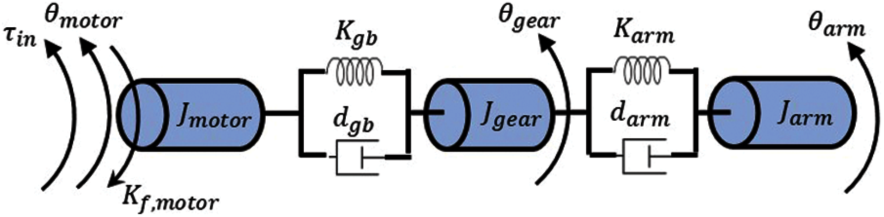
Figure 1: The model of the nonlinear robot arm
The nonlinear torque friction part is considered as the effect of coulomb friction and Striebeck effect. The coulomb friction is assumed as [27].
The total nonlinear torque friction effect is considered as Tustin friction model [28]:
where
Applying newton second law, the equation of motion for the motor inertia, gear inertia, and arm inertia is
Respectively. To get the state space model, assume the following state variables:
The differential states from Eqs. (7)–(12) and the output formula, i.e., the angular velocity of the motor, can be arranged in state space model format as
where
The obtained state model in Eq. (13) will be implemented in the next section to be represented by the T-SFM approach. The numerical results of this study are based on the physical parameters of the robot model presented in Tab. 1.
After deriving the state equations of our proposed nonlinear robot model, T-SFM can be implemented to linearize the robot system as explained in the next section.
T-SFM is implemented to represent the nonlinear state space model of the robot arm. In addition, the T-SFM has linearized the nonlinear terms in state space equations. The nonlinear robot arm model will be denoted by T-SFM as
where
Under our considered range values, the minimum and maximum values of
where
these membership functions
The presented design of the controller is closely related to the feature of the derived T-SFM in the previous section. This feature is that the terms of state equations
Model rule 1
If
Model rule 2
If
Model rule 3
If
Model rule 4
If
Model rule 5
If
Model rule 6
If
Model rule 7
If
Model rule 8
If
Model rule 9
If
Model rule 10
If
Model rule 11
If
Model rule 12
If
Model rule 13
If
Model rule 14
If
Model rule 15
If
Model rule 16
If
In this way, the nonlinear robot model can be described in the following general formula
Applying the defuzzification principle of fuzzy method, the output of the system is obtained as:
where
For the obtained T-S fuzzy model rule, the technique of state feedback is applied to develop the following control rules
The PDC technique is implemented in this study to find the solution of the system using the obtained T-SFM. Considering Eqs. (29) and (33), PDC technique is applied to design the controller based on T-S fuzzy approach as follow
Our developed mode rules in Eq. (29) can be asymptotically stable by a potential positive matrix Q when satisfying the following conditions:
where
In this section, simulation tests with MatLab R2017b are implemented to verify the performance of the designed controller for the robot arm model of the parameters that are listed in Tab. 1 with initial arm position and angular velocity
where
•
•
•
•
•
•
•
•
•
•
•
•
•
•
•
One of the essential considerations of LMI design is the interconnection of membership
Referring to Eq. (41), T-SFM controller has been designed by applying PDC technique
where
The simulation results of the proposed model are shown in Figs. 2 and 3. In Fig. 2, the results of the robot arm position and velocity are presented for the equilibrium situation where
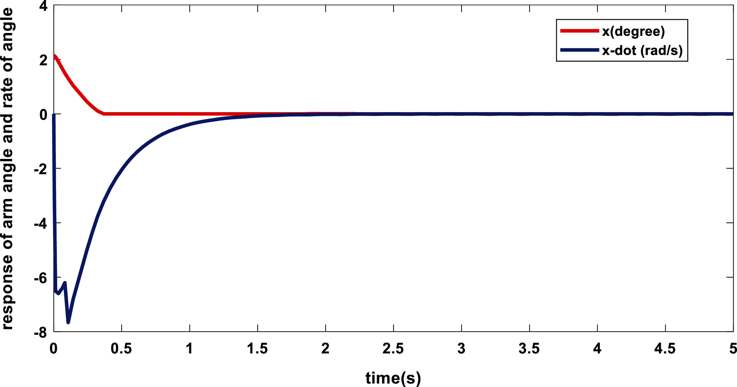
Figure 2: States of arm response
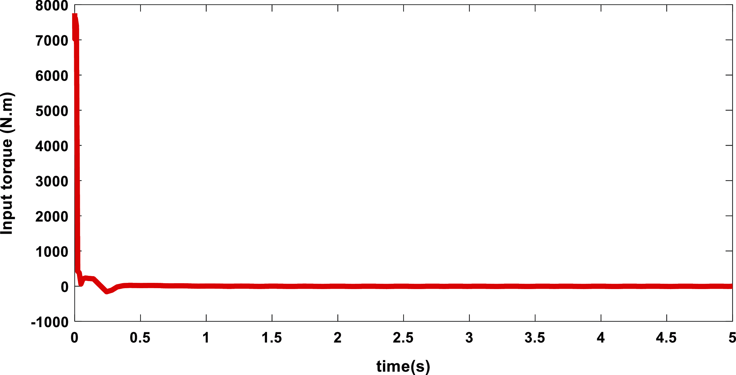
Figure 3: Input torque of motor
In this paper, a new control technique of the rotation motion of a nonlinear robot arm manipulator is introduced. The LMI and PDC control approaches are implemented based on TS-FM of the state space equations. The TS-FM has been developed for linearizing the nonlinear parameters in the state space equations in appropriately selected conditions of the operating points. The prime concept of the designed controller is to deduce all the fuzzy rules using the PDC approach in order to compensate for all rules of the fuzzy model. Furthermore, the linear matrix inequalities (LMIs) are applied to generate adequate cases for approving the stability and control purpose issues. The simulation results demonstrate that the proposed control technique stabilized the system with zero tracking error in less than 1.5 s. This is a suitable control performance for nonlinear robot arm models. The main limitation of this work is the non-utilization of optimization techniques such as genetic algorithms to find the optimum boundaries of membership functions that minimize the tracking errors. This will be addressed in the future by using such approaches to deal with the design membership functions in this application considering their types and boundaries.
Funding Statement: The authors received no specific funding for this research study.
Conflicts of Interest: The authors declare that they have no conflicts of interest to report regarding the present study.
1. A. D. Luca and W. J. Book, Robots with flexible elements. In: Springer Handbook of Robotics, 1st ed., Berlin, Heidelberg: Springer, pp. 243–282, 2016. [Google Scholar]
2. M. Wojtyra, “Modeling of static friction in closed-loop kinematic chains-uniqueness and parametric sensitivity problems,” Multibody System Dynamics, vol. 39, no. 4, pp. 337–361, 2017. [Google Scholar]
3. O. S. Solaiman, S. Ariffin and I. Hashim, “Dynamical comparison of several third-order iterative methods for nonlinear equations,” Computers, Materials & Continua, vol. 67, no. 2, pp. 1951–1962, 2021. [Google Scholar]
4. A. A. Hamad, A. S. Al-Obeidi, E. H. Al-Taiy, O. I. Khalaf and D. Le, “Synchronization phenomena investigation of a new nonlinear dynamical system 4D by Gardano’s and Lyapunov’s methods,” Computers, Materials & Continua, vol. 66, no. 3, pp. 3311–3327, 2021. [Google Scholar]
5. S. A. Sariman and I. Hashim, “New optimal Newton-householder methods for solving nonlinear equations and their dynamics,” Computers, Materials & Continua, vol. 65, no. 1, pp. 69–85, 2020. [Google Scholar]
6. C. Ku and W. Yeih, “Dynamical Newton-like methods with adaptive stepsize for solving nonlinear algebraic equations,” Computers, Materials & Continua, vol. 31, no. 3, pp. 173–200, 2012. [Google Scholar]
7. Z. Sun, Y. Bi, S. Chen, B. Hu, F. Xiang et al., “Designing and optimization of fuzzy sliding mode controller for nonlinear systems,” Computers, Materials & Continua, vol. 61, no. 1, pp. 119–128, 2019. [Google Scholar]
8. M. Chu, Q. Jia and H. Sun, “Backstepping control for flexible joint with friction using wavelet neural networks and L2-gain approach,” Asian Journal of Control, vol. 20, no. 2, pp. 856–866, 2018. [Google Scholar]
9. T. Ren, T. Dong, D. Wu and K. Chen, “Impedance control of collaborative robots based on joint torque servo with active disturbance rejection,” Industrial Robot: The International Journal of Robotics Research and Application, vol. 46, no. 4, pp. 518–528, 2019. [Google Scholar]
10. S. Amirkhani, S. Mobayen, N. Iliaee, O. Boubaker and S. H. Hosseinnia, “Fast terminal sliding mode tracking control of nonlinear uncertain mass-spring system with experimental verifications,” International Journal of Advanced Robotic Systems, vol. 16, no. 1, pp. 1729881419828176, 2019. [Google Scholar]
11. A. Benzaouia and A. E. Hajjaji, Advanced Takagi–Sugeno systems: Delay and saturation. In: Studies in Systems, Decision and Control, 1st ed., vol. 8. Switzerland: Springer International Publishing, 2014. [Google Scholar]
12. M. Namazov and A. Alili, “Stable and optimal controller design for Takagi–Sugeno fuzzy model based control systems via linear matrix inequalities,” in Proc. of Int.Conf. on Automatics and Informatics, Sofia, Bulgaria, pp. 69–72, 2016. [Google Scholar]
13. J. Liu, Intelligent Control Design and Matlab Simulation, 1st ed., Singapore: Springer, 2018. [Google Scholar]
14. L. Chaouech and A. Chaari, “Design of sliding mode control of nonlinear system based on Takagi–Sugeno fuzzy model,” in World Congress on Computer and Information Technology (WCCITSousse, Tunisia, pp. 1–6, 2013. [Google Scholar]
15. X. Song, M. Wang, Q. Zhang, S. Song and Z. Wang, “Takagi–Sugeno fuzzy model based event triggered point control for semilinear partial differential equation systems using collocated pointwise measurements,” International Journal of Robust and Nonlinear Control, vol. 31, no. 4, pp. 1122–1144, 2021. [Google Scholar]
16. P. Hušek and K. Narenathreyas, “Aircraft longitudinal motion control based on Takagi–Sugeno fuzzy model,” Applied Soft Computing, vol. 49, pp. 269–278, 2016. [Google Scholar]
17. X. Tang, D. Ning, H. Du, W. Li and W. Wen, “Takagi–Sugeno fuzzy model-based semi-active control for the seat suspension with an electrorheological damper,” IEEE Access, vol. 8, pp. 98027–98037, 2020. [Google Scholar]
18. A. V. Hemeyine, A. Abbou, N. Tidjani, M. Mokhlis and A. Bakouri, “Robust Takagi–Sugeno fuzzy models control for a variable speed wind turbine based a DFI-generator,” International Journal of Intelligent Engineering and Systems, vol. 13, no. 3, pp. 90–100, 2020. [Google Scholar]
19. L. Cheng, W. Liu, Z. Hou, T. Huang, J. Yu et al., “An adaptive Takagi–Sugeno fuzzy Model-based predictive controller for piezoelectric actuators,” IEEE Transactions on Industrial Electronics, vol. 64, no. 4, pp. 3048–3058, 2017. [Google Scholar]
20. Y. C. Lin, V. E. Balas, J. F. Yang and Y. H. Chang, “Adaptive Takagi–Sugeno fuzzy model predictive control for permanent magnet synchronous generator-based hydrokinetic turbine systems,” Energies, vol. 13, no. 20, pp. 5296, 2020. [Google Scholar]
21. C. H. Chiu and Y. F. Peng, “Design of Takagi–Sugeno fuzzy control scheme for real world system control,” Sustainability, vol. 11, no. 14, pp. 3855, 2019. [Google Scholar]
22. X. Zhu and W. Li, “Takagi–Sugeno fuzzy model based shaft torque estimation for integrated motor-transmission system,” ISA Transactions, vol. 93, pp. 14–22, 2019. [Google Scholar]
23. I. Al-Darraji, M. Derbali, H. Jerbi, F. Q. Khan, S. Jan et al., “A technical framework for selection of autonomous uav navigation technologies and sensors,” Computers, Materials & Continua, vol. 68, no. 2, pp. 2771–2790, 2021. [Google Scholar]
24. I. Al-Darraji, D. Piromalis, A. A. Kakei, F. Q. Khan, M. Stojmenovic et al., “Adaptive robust controller design-based RBF neural network for aerial robot arm model,” Electronics, vol. 10, no. 7, pp. 831, 2021. [Google Scholar]
25. I. Al-Darraji, M. Derbali and G. Tsaramirsis, “Tilting-rotors quadcopters: A new dynamics modelling and simulation based on the Newton–Euler method with lead compensator control,” in Proc. of 8th Int. Conf. on Computing for Sustainable Global Development (INDIAComNew Delhi, India, pp. 363–369, 2021. [Google Scholar]
26. E. Wernholt and S. Gunnarsson, “Nonlinear identification of a physically parameterized robot model 1,” IFAC Proceedings, vol. 39, no. 1, pp. 143–148, 2006. [Google Scholar]
27. G. Ellis, Nonlinear behavior and time variation. In: Control System Design Guide: Using Your Computer to Understand and Diagnose Feedback Controllers, 4th ed., Waltham, USA: Butterworth-Heinemann, pp. 235–259, 2012. [Online]. Available at: https://www.sciencedirect.com/book/9780123859204/control-system-design-guide. [Google Scholar]
28. L. Márton and B. Lantos, “Identification and model-based compensation of striebeck friction,” Acta Polytechnica Hungarica, vol. 3, no. 3, pp. 45–58, 2006. [Google Scholar]
 | This work is licensed under a Creative Commons Attribution 4.0 International License, which permits unrestricted use, distribution, and reproduction in any medium, provided the original work is properly cited. |