[BACK]
Computers, Materials & Continua
DOI:10.32604/cmc.2022.013906 |  |
| Article | |
Structure Preserving Algorithm for Fractional Order Mathematical Model of COVID-19
Zafar Iqbal1,2, Muhammad Aziz-ur Rehman1, Nauman Ahmed1,2, Ali Raza3,4, Muhammad Rafiq5, Ilyas Khan6,* and Kottakkaran Sooppy Nisar7
1Department of Mathematics, University of Management and Technology, Lahore, Pakistan
2Department of Mathematics and Statistics, The University of Lahore, Lahore, Pakistan
3Stochastic Analysis & Optimization Research Group, Department of Mathematics, Air University, Islamabad, 44000, Pakistan
4Department of Mathematics, National College of Business Administration and Economics, Lahore, Pakistan
5Department of Mathematics, Faculty of Sciences, University of Central Punjab, Lahore, 54500, Pakistan
6Faculty of Mathematics and Statistics, Ton Duc Thang University, Ho Chi Minh City, 72915, Vietnam
7Department of Mathematics, College of Arts and Science at Wadi Aldawaser, Prince Sattam Bin Abdulaziz University, Alkharj, 11991, Kingdom of Saudi Arabia
*Corresponding Author: Ilyas Khan. Email: ilyaskhan@tdtu.edu.vn
Received: 30 August 2021; Accepted: 10 November 2021
Abstract: In this article, a brief biological structure and some basic properties of COVID-19 are described. A classical integer order model is modified and converted into a fractional order model with ξ as order of the fractional derivative. Moreover, a valued structure preserving the numerical design, coined as Grunwald–Letnikov non-standard finite difference scheme, is developed for the fractional COVID-19 model. Taking into account the importance of the positivity and boundedness of the state variables, some productive results have been proved to ensure these essential features. Stability of the model at a corona free and a corona existing equilibrium points is investigated on the basis of Eigen values. The Routh–Hurwitz criterion is applied for the local stability analysis. An appropriate example with fitted and estimated set of parametric values is presented for the simulations. Graphical solutions are displayed for the chosen values of ξ (fractional order of the derivatives). The role of quarantined policy is also determined gradually to highlight its significance and relevancy in controlling infectious diseases. In the end, outcomes of the study are presented.
Keywords: Coronavirus pandemic model; deterministic ordinary differential equations; numerical methods; convergence analysis
1 Introduction (COVID-19)
Novel coronavirus is a spherical or pleomorphic shaped, particle having single stranded (positive sense) RNA (Ribonucleic Acid) linked to a nucleoprotein surrounded by a special type of protein. The outer surface of the coronavirus contains the projections of the club-shaped structure. The Classification of the coronaviruses depends upon the appearance of the outer surface (whether it is crown like or halo like), the replication mechanism and the distinct features related to the chemistry of the virus. In general, these viruses belong to OC43-like or 229E-like serotypes. Avian and mammalian species serve as hosts for them. Both types are similar with respect to morphology and chemical structure. Corona viruses present in human beings and animals are antigenically similar. These are capable of attacking on different types of tissues in animals. But, in human beings this family of viruses generally cause only the upper respiratory tract infection. This virus belons to the subclass Orthocoronavirinae, class Coronaviridae, order Nidovirales, realm Riboviria, kingdom Orthcornavirae and phylum Pisuviricota. The dimension of this virus varies from 26 to 32 kilobases, which is largest in the class of RNA viruses. They have distinct protruded club or clove shaped studs or spikes [1]. Like other corona viruses, COVID-19 also contains protein in the form of spikes ejecting outside from the surface. These spikes cling with the host (human) cells then its genome bears a structural change and the viral membrane fuse with the host cell cytoplasm. After this step, the viral genes of the COVID-19 enter into the host cell for replication and multiplication of the viruses. Depending upon the protease of the host cell, cleavage reaction permits it to reach into the host cell by endocytosis or fusion. After entering into the host cell, the virus becomes uncovered and their genome attacks on the cell cytoplasm. The genome of the coronavirus works as a messenger and it is translated by the ribosomes of the host cells. These viruses are divided into four categories as alpha coronavirus, beta coronavirus, gamma coronavirus and delta coronavirus. The first two viruses infect the mammals while the last two viruses initially attack the birds. The genera and species of these viruses are described as follows: the species Alphacoronavirus 1, Human coronavirus 229E, Human coronavirus NL63, Miniopterus bat coronavirus 1, Miniopterus bat cor onavirus HKU8, Porcine epidemic diarrhea virus, Rhinolophus bat coronavirus HKU2 and Scotophilus bat coronavirus 512 belong to the Alpha coronavirus. While the species, Betacoronavirus 1(Bovine Coronavirus, Human coronavirus OC43), Hedgehog coronavirus 1, Human coronavirus HKU1, Middle East respiratory syndrome-related coronavirus, Murine coronavirus, Pipistrellus bat coronavirus HKU5, Rousetlus bat coronavirus HKU9, Severe acute respiratory syndrome- related coronavirus (SARS-Cov, SARS-Cov-2) and Tylonycteris bat coronavirus HKU4 belong to Beta coronavirus. Furthermore, the species Avian coronavirus and Beluga whale coronavirus SW1 are the members of the Gamma coronavirus. Lastly, the Bulbul coronavirus HKU11 and Porcine coronavirus HKU15 species are the family members of the Delta coronavirus. Coronaviruses are deleterious to health with high risk factor. Some of them have more than 30% mortality rate, for instance MERS-COV. But other are not so harmful like as common cold. All types of the coronaviruses can be the causative agent of cold with prime symptoms including fever, sore throat and swollen adenoids. Moreover, they can cause primary viral pneumonia or secondary bacterial pneumonia or bronchitis in the same way as that of pneumonia [2]. The SARS-COV appeared in 2003, resulted in severe acute respiratory syndrome (SARS). It effected both the upper and lower respiratory tract due to an unmatched pathogenesis. There are six classes of human coronaviruses that are known so far, each specie is categorized into two types. There are seven types of human coronaviruses. Four coronaviruses which show mild symptoms are: Human coronavirus OC43 (HCOV-OC43), β-Cov, Human coronavirus HKU1 (HCOV-HKU1) and β-Cov, Human coronavirus 229E (HCOV-229E), α-Cov, Human coronavirus NL63 (HCOV-NL63) and α-Cov. Three coronaviruses which show severe symptoms are middle east respiratory syndrome-related coronavirus (MERS-COV), β-Cov, Severe acute respiratory syndrome coronavirus (SARS-COV), β-Cov and Severe acute respiratory syndrome coronavirus-2 (SARS-COV-2) and β-Cov. The HCOV-OC43, HCOV-HKU1, HCOV-229E and HCOV-NL63. They periodically produce the mild symptoms of the common cold in the population all around the year. The outburst of pneumonia in Wuhan, China declared a pandemic by WHO (World Health Organization). This is considered due to a novel type of coronavirus, provisionally named as 2019-nCov by WHO, later it was renamed as SARS-COV-2 by the international committee on Taxonomy of viruses. As of 24 June 2020, 476,911 deaths and more than 9,237691 confirmed cases of COVID-19 were recorded. The Wuhan breed is recognized as a new class of Beta coronavirus, which is genetically similar to SARS-COV. Since COVID-19 has a great resemblance with the bat coronavirus so it is suspected to be initiated from bats also [3]. As there is no vaccination or treatment for this disease so it has become a challenge for the scientists, health workers and policy makers to control the spreading of the infection. However, the research community and scientists are making efforts to find the treatment, vaccine or factors that are helpful in slowing down the dynamics of the disease. As a matter of fact, the virus is new however the virus family is not new for the human beings. The humanity has already faced such types of viruses on different scales in the near past. Currently, this infection has frozen all types of academic, business, sports and many other routine activities which created many problems and difficulties for the human beings as well as for the society [4]. The eradication of the COVID-19 is an uphill task for the relevant authorities. The modern world is fighting against the infectious diseases on the one hand and changing environmental conditions that are favorable for the emergence of the viral diseases on the other hand. The examination of dead bodies revealed that most of the patients were diagnosed with severe heart, lungs, diabetes and some other diseases. The Disease can be communicated easily through the nasal viral secretion that is transmitted directly or indirectly to the susceptible person. Generally, the symptoms of the infection are mild but in some cases painful death is also observed. The effective forecast for the disease dynamics is a prolific study matter regarding epidemiology, mathematical modeling and simulations. There exist many classes of mathematical models that depend upon the assumptions imposed on the process of dynamics. For instance, SIS, SIR, SEIR, SEIQR and many other compartmental models are used to formulate nonlinear incidence rates and double epidemic hypothesis [5]. In these types of models S,E,I,Q and R describe the susceptible, exposed, infected, quarantined and recovered individuals. These cellular or compartmental systems are used for adjusted incidence rate and imperfect vaccinations [6]. In these models, it is assumed that the susceptible individuals are aware of the infection’s presence [7]. It is worth mentioning that most of the existing deterministic models rest on the ordinary differential equations which imply the assumption of constant diffusion in the domain population. On the other hand, the use of partial differential equations model highlights the non-constant diffusion of the infection [8–10]. Although, many studies have been carried out for the providing the deeper insight into the disease dynamics. Chen et al. [11] considered a model with four compartments to investigate the dynamics of the novel infection. Shim and co-authors [12] addressed the questions relating to the effect analysis of the disease. Naveed et al. [13] developed a mathematical model to analyze the virus communication among the population and calculated the basic reproductive number. Many other approaches on the infection propagation may be seen in the sequel. Fractional calculus (FC) is the extension of the integer order calculus. On the basis of FC, the researchers are trying to understand the real world phenomenon of the infectious diseases in a more comprehensive way. They are developing mathematical models with derivatives of non-integer order. By the usage of these types of fractional operators many fruitful studies have been made in the recent scenario. New features and properties of the FC have fascinated the researchers, engineers and scientists to model the problems in the frame work of fractional calculus. The development of new non integer order operators have brought a number of essential features of many physical problems in to the lime light. The history of non-integer order calculus starts with a question posed by Leibniz in 1965. There is a long list of existing fractional order differential operators depending upon the nature of Kernels. Caputo, Riemann–Liouvelle and Katugampola fractional differential operators are developed by using singular kernels. While the fractional operators without singular kernels are of two types. In first type, exponential kernel is used for instance, Caputo–Fabrizio fractional differential operator. Whereas Mittag-Leffler kernel is used in the second type of operators e.g., Atangana–Baleanu fractional operator in Caputo sense. Due to the salient features of the FC, it is used to model a wide range of physical and dynamical problems in various fields of physical sciences, mathematics, life sciences and engineering [14]. Positivity, boundedness and the stability of the equilibrium points for the fractional order physical problems is a challenging task for the scientists and mathematicians. Some researchers are working in this line, but a lot of work is still to be done. Memory effect and hereditary properties are among the celebrated features of the non-integer order derivatives that are helpful in describing the disease dynamics. Taking in to account the memory effect, the fractional order models provide all the important informations from the past that are helpful in forecasting the dynamics of the infection more accurately and comprehensively. Saeedian and co-authors [15] designed a fractional SIR infectious disease model with memory effect and investigated the infection spread in the population. Ucar et al. [16] studied the dynamics of a fractional order smoking model. In the current study, an integer order model is considered initially then we switched on the non-integer order model by using Caputo differential operator. The fractional order model of COVID-19 can describe the complex dynamics of the physical phenomena with a more realistic approach.
2 Preliminaries
In this section, we will present some fundamental definitions of non-integer order derivatives, their key properties and notations used in this article.
2.1 Non Integer Order Derivatives
Fractional order derivatives have been defined by many researchers in a number of ways according to the nature of the kernel used therein. Some basic fractional order operators are defined in this section. Firstly, the Riemann–Liouville non integer order derivative of order 0<ξ≤1 is defined as,
RLD0ξϕ(t)=1Γ(k−ξ)dkdtk∫0tϕ(s)(t−s)k−ξ−1ds(1)
where k=[ξ]+1,k−1<ξ≤k,dkdtk is the kth order derivative and Γ(.) is the extensively used gamma function presented by Euler Fractional order derivative of a function is not defined in a unique way, as in the classical calculus an integer order derivative of a function is defined. Fractional derivative is a generic name given to a class of differential operators used to find the non-integer order derivative of a function. These operators are defined by a number of researchers in different ways. Some of them are Liouville, Riemann–Liouville, Caputo, Fabrizio, Grunwald–Letnikov and many more can be studied in the sequel. Among many other questions, it is important that which differential operator best suits for the underlying model. A more generic fractional operator should be selected for the purpose. The Caputo fractional operator is defined as,
0CD0ξϕ(t)=1Γ(k−ξ)∫0t(t−s)k−ξ−1dkdtkf(s)ds. (2)
The importance of this operator, when applied to solve a system of fractional differential equations is that it can be associated with initial conditions of classical order, which results in an initial value problem in the desired form as,
0CD0ξϕ(t)=ϕ(t,y(t)),Dy(t0)=y0k,k=1,2,3,…,n−1
A very useful definition relating to this article by using the classical finite differences on a uniform mesh partionised in [0,t] is described as follows, consider that Dtξϕ(t) observes the particular smoothness constraints in every interval (0,t),t≤T with mesh points as
0=τ0<τ1<…<τn+1=t=(n+1)h
where h is defined as the difference of τn+1 and τn. By using the classical finite difference symbols, we have
1hξΔhξϕ(t)=1hξ(ϕ(τn+1)−∑i=1n+1eiξϕ(τn+1−i))
where eiξ=(−1)i−1(ξi) and the by Grunwald Letnikov approximation is given as
Dtξϕ(t)=limh→01hξΔhξϕ(t) (3)
This expression is derived from the famous Euler method. Consider the fractional differential equation
0CD0ξϕ(t)=f(ϕ(t),ϕ(τ)) (4)
Now, by applying the G-L scheme on a uniform mesh, we obtain the following expression
ϕn+1−∑i=1n+1−γn+1ϕ0=hξf(ϕm), (5)
where e and γn satisfy the following relations ei=(−1)i−1(ξi) and
γn=hξγ0(τn+1)=γ0,−1(n+1)−ξ, where the coefficient on the right hand side is described as
γ0,−1=Γ(µξ+1)Γ(kξ+1),
where μ,kϵN∪{0}.
Furthermore, ei and γi observe the relations as stated in the Lemma 1.
Lemma 1 [17]: Let 0<ξ<1, then the coefficients expressed by
ei=(−1)i−1(ξi) are positive and obey the relation
ei=O(1e1+ξ) as i→∞.
Also the following two relations are satisfied
0≤er+1<er…<e1=ξ<1
and 0≤γi+1<γi…<γ1=1Γ(1−ξ)
In this section, we present the GL-NSFD hybrid scheme is formulated by combining the GL scheme for numerical approximation of the fractional order derivatives and NSFD scheme constructed by using the standard rules designed by Mickens. More details can be seen in [18]. The system of equations for COVID-19 is described as follows:
0CD0ξS(t)=λξ−(β1ξI(t)+β2ξE(t))S(t)−μξS(t) (6)
0CD0ξE(t)=(β1ξI(t)+β2ξE(t))S(t)−(q1ξ+kξ+αξ+μξ)E(t) (7)
0CD0ξI(t)=αξE(t)−(rξ+μξ+d1ξ)I(t) (8)
0CD0ξQ(t)=q1ξE(t)−(qξ+μξ+d2ξ)Q(t) (9)
0CD0ξR(t)=kξE(t)+rξI(t)+qξQ(t)−μξR(t) (10)
2.2 GL-NSFD Scheme
In this portion, we will construct the proposed scheme. The discretization of fractional derivative C0D0ξS(t) is given as,
0CD0ξS(t)=1ϕ(h)ξ(Sn+1−∑i=1n+1eiSn+1−i−rn+1So).
The above formula is used on the left hand side of Eq. (6) to get the following expression
Sn+1−∑i=1n+1eiSn+1−i−rn+1So=ϕ(h)ξλξ−ϕ(h)ξβ1ξIn(t)Sn+1(t)−ϕ(h)ξβ2ξEnSn+1−ϕ(h)ξμξSn+1.
After some simplifications, we have the final form as,
Sn+1=∑i=1n+1eiSn+1−i+rn+1So+ϕ(h)ξλξ1+ϕ(h)ξ[β1ξIn+β2ξEn+μξ] (11)
Similar procedure is adopted for the remaining compartments and we have the final forms as,
En+1=∑i=1n+1eiEn+1−i+rn+1Eo+ϕ(h)ξ[β1ξIn+β2ξEn]Sn1+ϕ(h)ξ(q1ξ+kξ+μξ+αξ) (12)
In+1=∑i=1n+1eiIn+1−i+rn+1Io+ϕ(h)ξαEn1+(rξ+μξ+d1ξ)ϕ(h)ξ (13)
Qn+1=∑i=1n+1eiQn+1−i+rn+1Qo+ϕ(h)ξq1ξEn1+(qξ+μξ+d2ξ)ϕ(h)ξ (14)
Rn+1=∑i=1n+1eiRn+1−i+roRo+ϕ(h)ξ[kξEn+rξIn+qξQn]1+μξϕ(h)ξ (15)
2.3 Positivity of the Solution
In this portion, positivity of the solution will be investigated. Positivity is an important feature of the compartmental models. Since, the state variables in these type of models describe the size of the population that cannot be negative. So, positivity is the basic requirement of the solutions at every moment of time. Following result is helpful in this regard.
Theorem: Assume that all the unknowns and parameters arose in the model are non-negative i.e., So,Eo,Io,Qo and Ro are positive. Also λξ,μξ,kξ,rξ,αξ,d1ξ,d2ξ,β1ξ,β2ξ,q1ξ,q2ξ,qξ and ϕ(h)ξ all are ≥0. Then Sn,En,In,Qn and Rn all are ≥0 ∀n∈Z+.
Proof: Taking in to account the Eqs. (11) to (15) for n = 0, we have
S1=e1So+r1So+ϕ(h)ξλξ1+ϕ(h)ξ(β1ξIo+β2ξE0+μξ)
From the restrictions imposed on the state variables and parameters, it is evident that S1≥0. Similarly, E1≥0,I1≥0,Q1≥0 and R1≥0. Continuing in the same way and by straight forward calculations, it is easy to conclude that Sn+1≥0,En+1≥0,In+1≥0,Qn+1≥0 and Rn+1≥0. i.e.,
Sn+1=∑i=1n+1eiSn+1−i+rn+1So+ϕ(h)ξλξ1+ϕ(h)ξ[β1ξIn+β2ξEn+μξ]≥0,En+1=∑i=1n+1eiEn+1−i+rn+1Eo+ϕ(h)ξ[β1ξIn+β2ξEn]Sn1++ϕ(h)ξ(q1ξ+kξ+μξ+αξ)≥0,
In+1=∑i=1n+1eiIn+1−i+rn+1Io+ϕ(h)ξαξEn1+(rξ+μξ+d1ξ)ϕ(h)ξ≥0,Qn+1=∑i=1n+1eiQn+1−i+rn+1Qo+ϕ(h)ξq1ξEn1+(qξ+μξ+d2ξ)ϕ(h)ξ≥0,
Rn+1=∑i=1n+1eiRn+1−i+roRo+ϕ(h)ξ[kξEn+rξIn+qξQn]1+μξϕ(h)ξ≥0.
2.4 Boundedness
Since the state variables in the model represent the subpopulation of a certain compartment. So the sum of values of all the state variables must be less than or equal to the total population or equivalently the sum of solutions at any time must be bounded. The following result is helpful in this regard.
Theorem: Let S0,E0,I0,Q0 and R0 are all finite quantities and S0 +E0 +I0 +Q0 +R0 = N0. Moreover, all the parameters involved in the model are positive. i.e., λξ,μξ,qξ,q1ξ,q2ξ,αξ,γξ,kξ and ϕ(h)ξ are positive, then there is a constant Bn+1 such that Sn+1≤Bn+1, En+1≤Bn+1,In+1≤Bn+1,Qn+1≤Bn+1,Rn+1≤Bn+1.
Proof: Considering the Eqs. (11) to (15), we have
Sn+1[1+ϕ(h)ξ(β1ξIn+β2ξEn+μξ)]+En+1[1++ϕ(h)ξ(q1ξ+kξ+μξ+αξ)]+In+1[1+ϕ(h)ξ(rξ+μξ+d1ξ)]+Qn+1[1+(qξ+μξ+d2ξ)ϕ(h)ξ]+Rn+1[1+μξϕ(h)ξ]=∑i=1n+1ei(Sn+1−i+En+1−i+In+1−i+Qn+1−i+Rn+1−i)+rn+1(So+Eo+Io+Qo+Ro)+ϕ(h)ξ[λξ+(β1ξIn+β2ξEn)Sn+(αξ+q1ξ+kξ)En+rξIn+qξQn] (16)
By applying the principle of mathematical induction,
for n = 0, we have
S1[1+ϕ(h)ξ(β1ξI0+β2ξE0+μξ)]+E1[1+ϕ(h)ξ(q1ξ+kξ+μξ+αξ)]+I1[1+ϕ(h)ξ(rξ+μξ+d1ξ)]+Q1[1+(qξ+μξ+d2ξ)ϕ(h)ξ]+R1[1+μξϕ(h)ξ]=e1N0+r1N0+ϕ(h)ξ[λ+(β1ξI0+β2ξE0)S0+(αξ+q1ξ+kξ)E0+rξI0+qξQ0]S1[1+ϕ(h)ξ(β1ξI0+β2ξE0+μξ)]≤(ξ+1Γ(1−ξ))N0+ϕ(h)ξ[λ+(β1ξ+β2ξ)I0S0+(αξ+q1ξ+kξ)E0+rξI0+qξQ0]=B1S1[1+ϕ(h)ξ(β1ξI0+β2ξE0+μξ)]≤B1S1≤B1as 1+ϕ(h)ξ(β1ξI0+β2ξE0+μξ)≥1
In the same way E1≤B1,I1≤B1,Q1≤B1 and R1≤B1.
Now, we calculate the expression (16) for n = 1, and obtain the following relations,
S2[1+ϕ(h)ξ(β1ξI1+β2ξE1+μξ)]+E2[1+ϕ(h)ξ(q1ξ+kξ+μξ+αξ)]+I2[1+ϕ(h)ξ(rξ+μξ+d1ξ)]+Q2[1+(qξ+μξ+d2ξ)ϕ(h)ξ]+R2[1+μξϕ(h)ξ]≤e1N1+(ξ+1Γ(1−ξ))N0+ϕ(h)ξ[λ+(β1ξI1+β2ξE1)S1+(αξ+q1ξ+kξ)E1+rξI1+qξQ1]=B2⟹S2[1+ϕ(h)ξ(β1ξI1+β2ξE1+μξ)]≤B2E2[1+ϕ(h)ξ(q1ξ+kξ+μξ+αξ)]≤B2I2[1+ϕ(h)ξ(rξ+μξ+d1ξ)]≤B2Q2[1+(qξ+μξ+d2ξ)ϕ(h)ξ]≤B2R2[1+μξϕ(h)ξ]≤B2
The above inequalities help us to reach at
S2≤B2as [1+ϕ(h)ξ(β1ξI1+β2ξE1+μξ)]≥1E2≤B2as [1+ϕ(h)ξ(q1ξ+kξ+μξ+αξ)]≥1I2≤B2as [1+ϕ(h)ξ(rξ+μξ+d1ξ)]≥1Q2≤B2as [1+(qξ+μξ+d2ξ)ϕ(h)ξ]≥1R2≤B2as [1+μξϕ(h)ξ]≥1
Now, let
Sm≤Bm,Em≤Bm,Im≤Bm,Qm≤BmandRm≤Bm
For some m∈Z+.
where,
Bm=5e1Bn−1+5e2Bn−2+…+(ξ+1Γ(1−ξ))N0+ϕ(h)ξ[λ+(β1ξIn−1+β2ξEn−1)Sn−1+(αξ+q1ξ+kξ)En−1+rξIn−1+qξQn−1]
Now for n∈Z+, we arrive at,
Sn+1[1+ϕ(h)ξ(β1ξIn+β2ξEn+μξ)]+En+1[1++ϕ(h)ξ(q1ξ+kξ+μξ+αξ)]+In+1[1+ϕ(h)ξ(rξ+μξ+d1ξ)]+Qn+1[1+(qξ+μξ+d2ξ)ϕ(h)ξ]+Rn+1[1+μξϕ(h)ξ]=e1(Sn+En+In+Qn+Rn)+e2(Sn−1+En−1+In−1+Qn−1+Rn−1)+e3(Sn−2+En−2+In−2+Qn−2+Rn−2)+…+en+1(S0+E0+I0+Q0+R0)+rn+1No+ϕ(h)ξ[λξ+(β1ξIn+β2ξEn)Sn+(αξ+q1ξ+kξ)En+rξIn+qξQn]Sn+1[1+ϕ(h)ξ(β1ξIn+β2ξEn+μξ)]+En+1[1+ϕ(h)ξ(q1ξ+kξ+μξ+αξ)]+In+1[1+ϕ(h)ξ(rξ+μξ+d1ξ)]+Qn+1[1+(qξ+μξ+d2ξ)ϕ(h)ξ]+Rn+1[1+μξϕ(h)ξ]≤e1(5Bn+5Bn−1+5Bn−2+…+5B1)+(ξ+1Γ(1−ξ))N0+ϕ(h)ξ[λξ+(β1ξIn+β2ξEn)Sn+(αξ+q1ξ+kξ)En+rξIn+qξQn]=Bn+1
In the same fashion a adopted before, we conclude that
Sn+1≤Bn+1,En+1≤Bn+1,In+1≤Bn+1,Qn+1≤Bn+1 and Rn+1≤Bn+1
So, the given expression is true for all positive values of n.
Hence, the solutions are bounded ∀n∈Z+.
2.5 Stability of the Model
In this portion, we will investigate the stability of the model at both the points of equilibria i.e., at a corona free equilibrium point and a corona existing equilibrium point.
The corona free equilibrium state of the model is given as C1=(λξμξ,0,0,0,0).
The corona virus existing equilibrium state is calculated as C2=(S1(t),E1(t),I1(t),Q1(t),R1(t)),
where, S1(t)=(q1ξ+kξ+μξ+αξ)(d1ξ+rξ+μξ)β1ξαξ+β2ξ(d1ξ+rξ+μξ), E1(t)=(λξ−μξS1(t))(d1ξ+rξ+μξ)(β1ξαξ+β2ξ(d1ξ+rξ+μξ))S1(t), I1(t)=αξE1(t)d1ξ+rξ+μξ, Q1(t)=q1ξE1(t)d2ξ+qξ+μξ, R1(t)=kξE1(t)+rξI1(t)+qξQ1(t)μξ.
Theorem: The corona free equilibrium C1=(So,Eo,Io,Qo,Ro)=(λξμξ,0,0,0,0) of the model is locally asymptotically stable if Ro<1, otherwise unstable for Ro>1.
Proof: The corona-free equilibrium C1=(So,Eo,Io,Qo,Ro)=(λξμξ,0,0,0,0) is locally asymptotically stable (LAS) if all the Eigenvalues λi<0,i=1,2,3,4,5 with condition |arg(λi)|>απ2. For the Eigen values, the Jacobean matrix at C1=(λξμξ,0,0,0,0) is given as follows:
J(C1)=[−μξβ2ξλξμξ−β1ξλξμξ000β2ξλξμξ−(kξ+αξ+μξ+q1ξ)β1ξλξμξ000αξ−(rξ+μξ+d1ξ)000q1ξ0−(qξ+μξ+d2ξ)00kξrξqξ−μξ]
Notice that the two Eigen values are repeated as λ1=−μξ<0,λ2=−μξ<0 and third Eigen value is
λ3=−(qξ+μξ+d2ξ)<0.
|J(C1)−λI|=|β2ξλξμξ−(kξ+αξ+μξ+q1ξ)−λ−β1ξλξμξαξ−(rξ+μξ+d1ξ)−λ|=0.
λ2+λ(−β2ξa1+a2+a3)+(a3a2−β2ξa1−αβ1ξa1)=0,
where, λξμξ=a1, (kξ+αξ+μξ+q1ξ)=a2 and (rξ+μξ+d1ξ)=a3.
By using the Routh–Hurwitz Criterion of 2nd order polynomial as,
a3+a2−β2ξa1>0, if(kξ+αξ+μξ+q1ξ)+(rξ+μξ+d1ξ)−β2ξλξμ>0,
R0=β2ξλξμξ(kξ+αξ+2μξ+q1ξ+rξ+d1ξ)<1 and (a3a2−β2ξa1−αξβ1ξa1)>0, when R0 < 1.
Hence, all Eigenvalues are negative and by Routh-Hurwitz criteria the given equilibrium point C1 is locally asymptotically stable.
Theorem: The corona existence equilibrium C2=(S1,E1,I1,Q1,R1) of the model is locally asymptotically stable if Ro>1, otherwise unstable for Ro<1.
Proof: The corona existence equilibrium C2=(S1,E1,I1,Q1,R1) is locally asymptotically stable (LAS) if all the Eigenvalues λi<0,i=1,2,3,4,5 with condition |arg(λi)|>απ2.
For the eigen values, the Jacobean matrix at C2=(S1,E1,I1,Q1,R1) is given as follows:
J(C2)=[−β1ξI1−β2ξE1−μξ−β2ξS1−β1ξS100β1ξI1+β2ξE1β2ξS1−(kξ+αξ+μξ+q1ξ)β1ξS1000αξ−(rξ+μξ+d1ξ)000q1ξ0−(qξ+μξ+d2ξ)00kξrξqξ−μξ]
Notice that, the Eigen values are λ1=−μξ<0 and λ2=−(qξ+μξ+d2ξ)<0
|J(C2)−λI|=|−b1−μξ−λ−b2−b4b1b2−b3−λb40αξ−b5−λ|=0.
λ3+(b1−b2+b3+b5+μξ)λ2+(b1b3+b1b5−b2b5+b3b5−b2μξ+b3μξ+b5μξ−b4αξ^)λ+(b1b3b5−b2b5μξ+b3b5μξ−b4αξμξ)=0.
where, b1=β1ξI1+β2ξE1+μξ, b2=−β2ξS1, b3=kξ+αξ+μξ+q1ξ, b4=β1ξS1, b5=rξ+μξ+d1ξ and b5=qξ+μξ+d2ξ.
By using the Routh–Hurwitz Criterion of 3rd order polynomial, we get the following expression:
(b1−b2+b3+b5+μξ)>0,(b1b3b5−b2b5μξ+b3b5μξ−b4αξμξ)>0, if R0 > 1,
and
(b1−b2+b3+b5+μξ)(b1b3+b1b5−b2b5+b3b5−b2μξ+b3μξ+b5μξ−b4αξ)>(b1b3b5−b2b5μξ+b3b5μξ−b4αξμξ), if R0 > 1.
Thus, we have concluded that all Eigenvalues are negative and by Routh Hurwitz criteria, the given equilibrium point C2 is locally asymptotically stable. Here, we will present a suitable numerical example and graphical solutions of the state variables involved in the model. This whole stuff is presented with the aid of computer simulations.
3 Numerical Example and Simulations
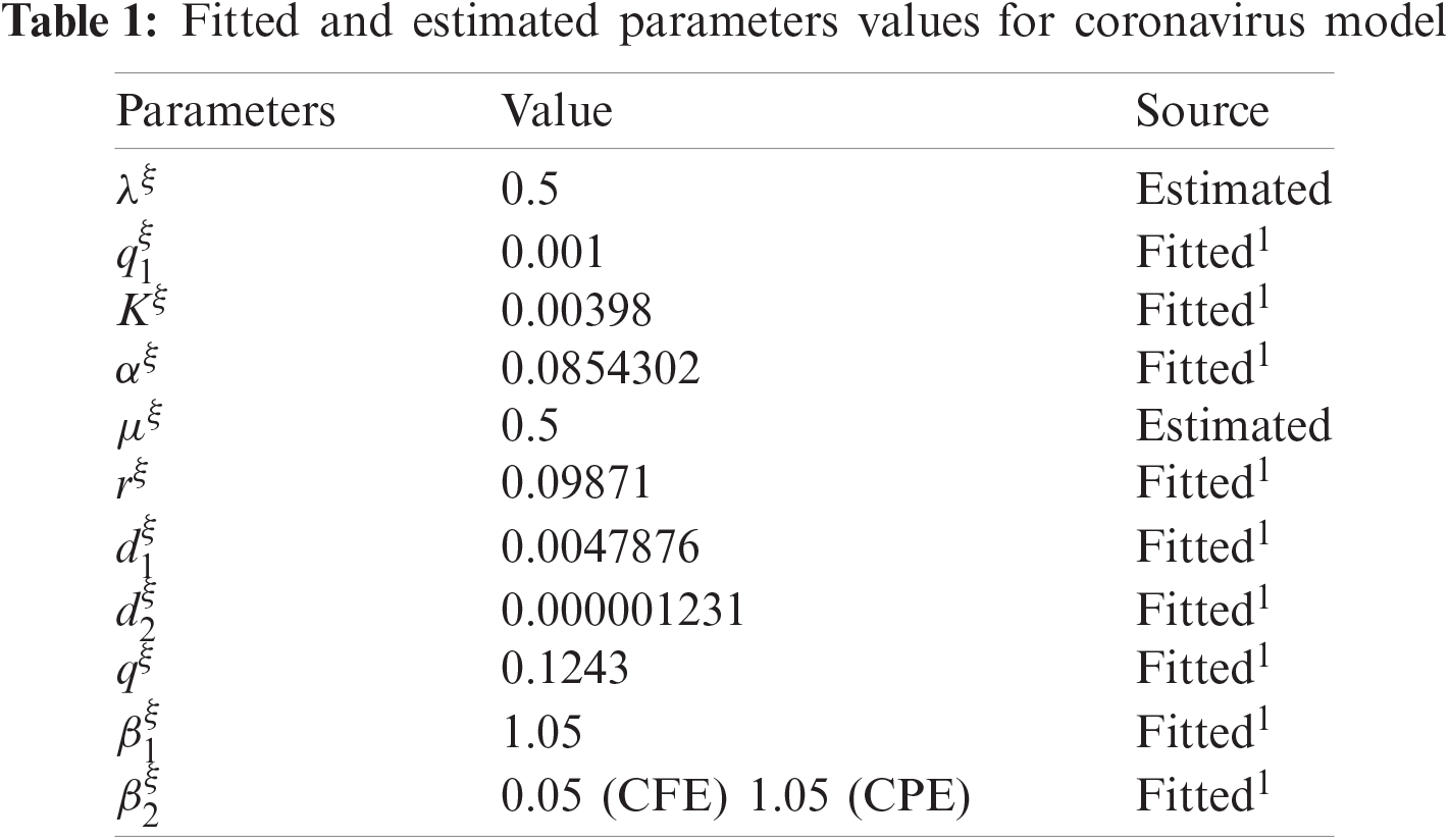
In this portion, an example of the fractional order COVID-19 model is provided. The parametric values are mentioned in Tab. 1. Also, non-negative initial conditions are considered.
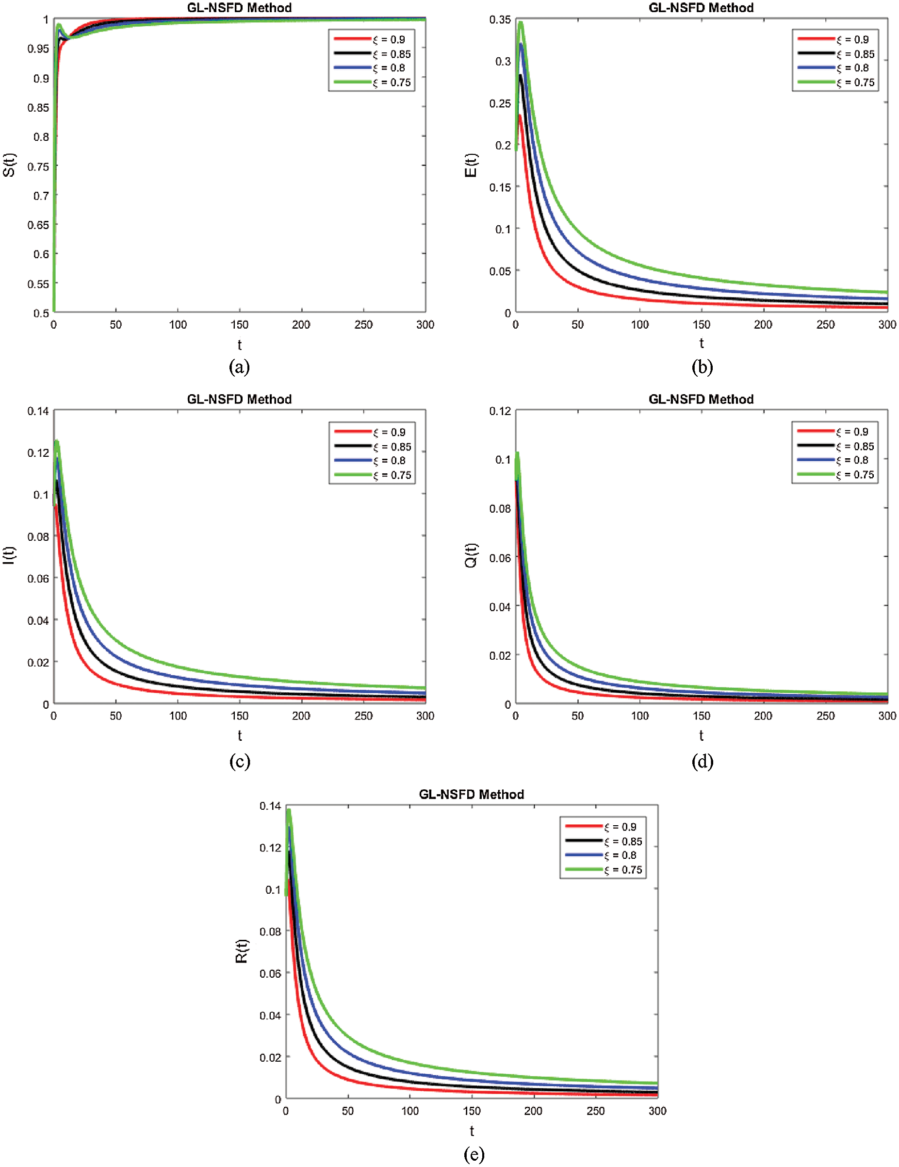
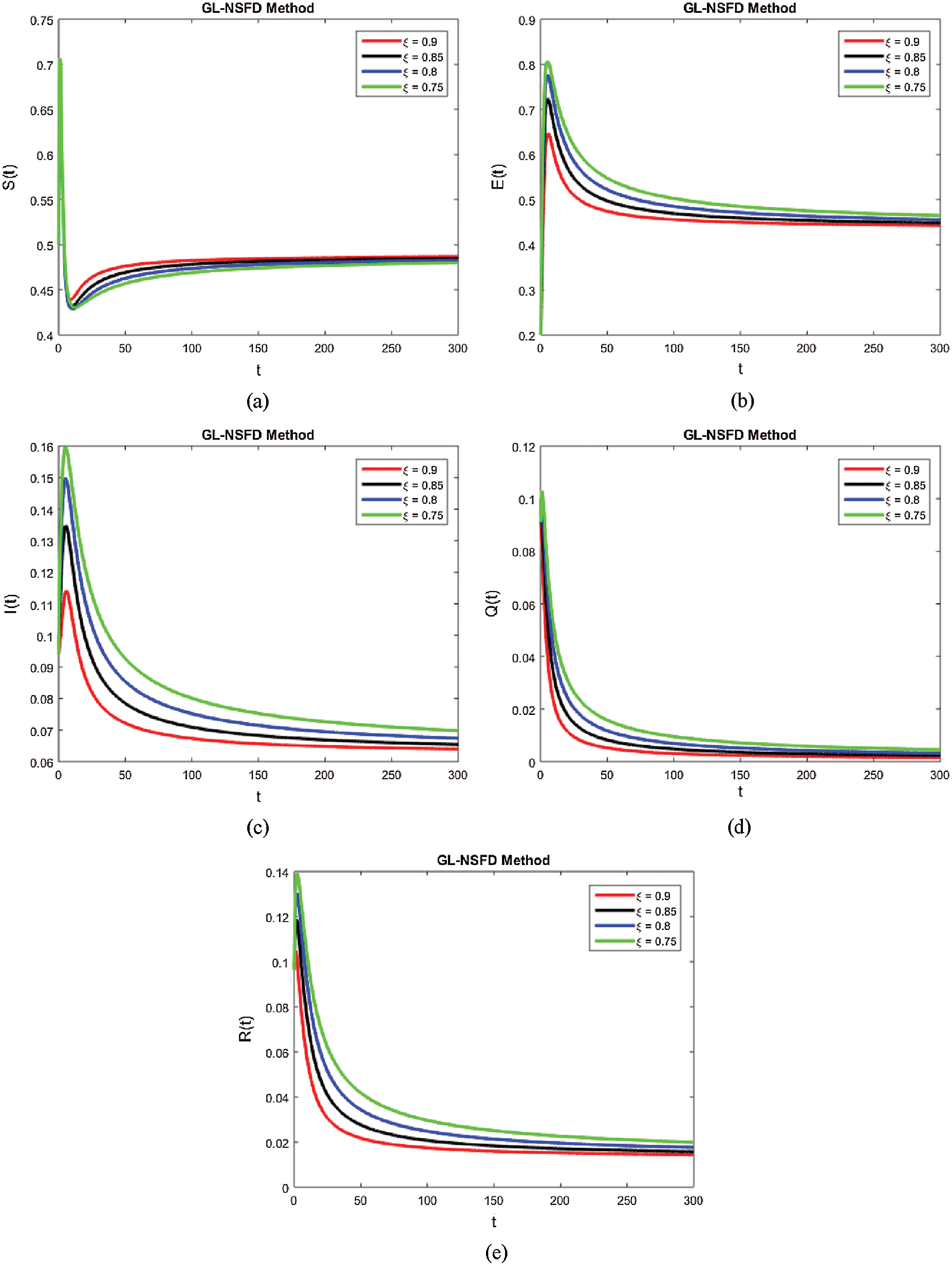
Computer aided graphs are submitted to support our assertions. These sketches support the fact that proposed numerical device is a structure preserving tool for solving the nonlinear fractional systems. The device encounters the positivity, stability and boundedness of the solutions. All the graphs in Fig. 1 reveals that all the subpopulations converge at the virus free equilibrium point (with different values of ξ). E1=(λξμξ,0,0,0,0) i.e., S(t)→λξμξ,E(t)→0,I(t)→0,Q(t)→0 and R(t)→0, when the population is infection free and the values of the parameters are chosen suitably as listed in Tab. 1. The graphs in Fig. 1 part (a) illustrate that all the curved trajectories representing the susceptible populace growing with time t approach towards the disease-free value of the susceptible individuals S(t)=λξμξ which is one in this case. Each trajectory is drawn against a certain value of ξ (the order of the fractional derivative) as mentioned in the figure. Moreover, the rate of the convergence towards the VFE of each trajectory is different, depending upon the value of ξ. Similarly, the other sketches in Fig. 1 part (b)–part (e) provide the strong evidence for our declaration about the proposed numerical design. The Fig. 2 exhibits the simulation results of our proposed scheme endemic equilibrium. The graphs (a), (b), (c), (d) and (e) in Fig. 2 provide the graphical solutions to S, E, I, Q and R for some selected values of ξ, where ξ is the fractional order of the derivative. The trajectories in Fig. 2 part (a) converge at the virus restricted state i.e., endemic state for different values of ξ, while the other parametric values are kept same as mentioned in Tab. 1. Each curved line in the graph Fig. 2 part (a) attains the equilibrium state of S1(t) which is represented as,
S1(t)=(q1ξ+kξ+μξ+αξ)(d1ξ+rξ+μξ)β1ξαξ+β2ξ(d1ξ+rξ+μξ),
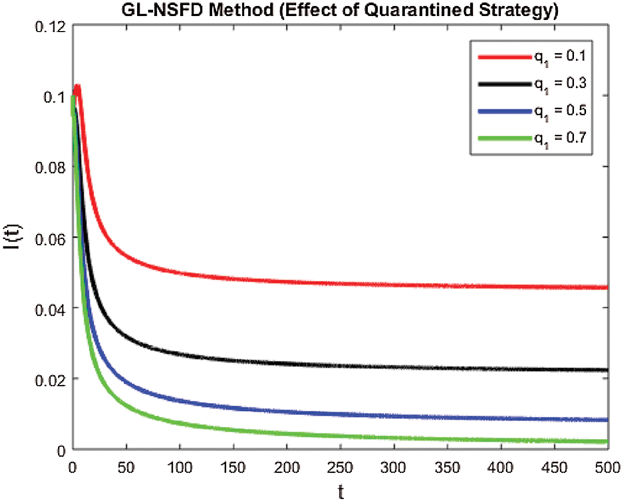
with a certain rate of convergence according to the value of ξ. Similarly, the other curved trajectories in Fig. 2 part (b)–part (e) depict that they attain the virus endemic equilibrium state for various values of ξ. The endemic equilibrium is expressed as (S1(t), E1(t), I1(t), Q1(t), R1(t)) and the value of each state variable is stated earlier in the section of the stability of the model. The Fig. 3 describes the quarantine approach to control the infection in the populace. The values of the quarantine factor q considered in this figure are as q1 = 0.1, q2 = 0.3, q3 = 0.5 and q4 = 0.7 while the ξ=0.9 is fixed. All the four curved representations in Fig. 3 unveil the key fact that by increasing the quarantine or isolation approach, the flock of infected individuals can be minimized to a certain level. In this area, we will submit the fruitful conclusion about the current study and some future directions will be pointed out.


Figure 1: The simulations results for all the subpopulations using proposed method at disease free equilibrium with the variation of fractional order ξ

Figure 2: The simulations results for all the subpopulations using proposed method at endemic free equilibrium with the variation of fractional order ξ

Figure 3: The effect of quarantined strategy on infected population by increasing the values of q1 for ξ=0.9
4 Conclusion
In this study, some biological and physical features of the novel corona virus-2019 are described. A classical SIEQR model is converted to fractional order compartmental model with ξ as order of the fractional derivatives. The GL-NSFD scheme is proposed to study the propagation of the COVID-19 along with some leading properties of the system. Moreover, the numerical study is made to ensure the pre-assumed results about the numerical design. The equilibrium points of the system are also described to detect the local stability of the model. The decisive role of R0 (reproductive number) in describing the stability of the system is also discussed. Positivity and boundedness of the numerical design is also investigated to exhibit the productiveness of the scheme. The computer-aided graphs are presented via computer simulations. These solutions coincide with the exact equilibrium points for different values of ξ. As, the proposed scheme preserves the structure of the system. So, it can be used successfully to solve many other non-linear physical systems. Moreover, this tool may be used to solve delay models, advection and diffusion reaction models in future.
Funding Statement: The authors received no specific funding for this study.
Conflicts of Interest: The authors declare that they have no conflicts of interest to report regarding the present study.
References
1. Y. Fan, K. Zhao, Z. L. Shi and P. Zhou, “Bat coronaviruses in China,” Viruses, vol. 11, no. 3, pp. 210–222, 2020. [Google Scholar]
2. B. W. Neuman, B. D. Adair, C. Yoshioka, J. D. Quispe, G. Orca et al., “Supramolecular architecture of severe acute respiratory syndrome coronavirus revealed by electron cry microscopy,” Journal of Virology, vol. 80, no. 16, pp. 7918–7928, 2020. [Google Scholar]
3. A. J. Kucharski, T. W. Russell, C. Diamond, Y. Liu, J. Edmunds et al., “Early dynamics of transmission and control of COVID -19: A mathematical modelling study,” Lancet Infectious Diseases, vol. 11, no. 2, pp. 1–17, 2020. [Google Scholar]
4. S. Zhao and H. Chen, “Modeling the epidemic dynamics and control of COVID-19 outbreak in China,” Quantitate Biology, vol. 11, no. 1, pp. 1–09, 2020. [Google Scholar]
5. X. Meng, S. Zhao, T. Feng and T. Zhang, “Dynamics of a novel nonlinear stochastic SIS epidemic model with double epidemic hypothesis,” Journal of Mathematical Analysis and Applications, vol. 433, no. 1, pp. 227–242, 2016. [Google Scholar]
6. F. Li, X. Meng and X. Wang, “Analysis and numerical simulations of a stochastic SEIQR epidemic system with quarantine-adjusted incidence and imperfect vaccination,” Computational and Mathematical Methods in Medicine, vol. 1, no. 1, pp. 1–19, 2018. [Google Scholar]
7. K. A. Kabir, K. Kuga and J. Tanimoto, “Analysis of SIR epidemic model with information spreading of awareness,” Chaos, Solitons & Fractals, vol. 119, no. 1, pp. 118–125, 2019. [Google Scholar]
8. S. Azam, J. E. Macias-Dıaz, N. Ahmed, I. Khan, M. S. Iqbal et al., “Numerical modeling and theoretical analysis of a nonlinear advection-reaction epidemic system,” Computer Methods and Programs in Biomedicine, vol. 1, no. 1, pp. 1–19, 2020. [Google Scholar]
9. J. E. Macıas-Dıaz, N. Ahmed and M. Rafiq, “Analysis and nonstandard numerical design of a discrete three-dimensional hepatitis b epidemic model,” Mathematics, vol. 7, no. 12, pp. 1–17, 2019. [Google Scholar]
10. N. Ahmed, M. Ali, M. Rafiq, I. Khan, K. S. Nisar et al., “A numerical efficient splitting method for the solution of two dimensional susceptible infected recovered epidemic model of whooping cough dynamics,” Computer Methods and Programs in Biomedicine, vol. 190, no. 1, pp. 1–18, 2020. [Google Scholar]
11. T. M. Chen, J. Rui, Q. P. Wang, Z. Y. Zhao, J. A. Cui et al., “A mathematical model for simulation the phase-based transmissibility of a novel coronavirus,” Infectious Diseases Poverty, vol. 9, no. 24, pp. 1–8, 2020. [Google Scholar]
12. E. Shim, A. Tariq, W. Choi and G. Chowell, “Transmission potential and severity of COVID-19 in South Korea,” International Journal of Infectious Diseases, vol. 17, no. 2, pp. 1–19, 2020. [Google Scholar]
13. M. Naveed, M. Rafiq, A. Raza, N. Ahmed, I. Khan et al., “Mathematical analysis of novel coronavirus (2019-nCov) delay pandemic model,” Computers, Materials and Continua, vol. 64, no. 3, pp. 1401–1414, 2020. [Google Scholar]
14. M. A. Khan and A. Atangana, “Modeling the dynamics of novel coronavirus (219-nCov) with fractional derivative,” Alexandria Engineering Journal, vol. 2, no. 33, pp. 1–11, 2020. [Google Scholar]
15. M. Saeedian, M. Khalighi, N. A. Tafreshi, G. R. Jafari and M. Ausloos, “Memory effects on epidemic evolution: The susceptible-infected-recovered epidemic model,” Physical Review E, vol. 95, no. 2, pp. 1–19, 2017. [Google Scholar]
16. S. Ucar, E. Ucar, N. Ozdemir and Z. Hammouch, “Mathematical analysis and numerical simulation for a smoking model with Atangana–Baleanu derivative,” Chaos Solitons & Fractals, vol. 118, no. 1, pp. 300–306, 2019. [Google Scholar]
17. R. Scherer, S. Kalla, Y. Tang and J. Huang, “The Grunwald–Letnikov method for fractional differential equations,” Computers and Mathematics with Application, vol. 62, no. 3, pp. 902–907, 2011. [Google Scholar]
18. R. E. Mickens, “A fundamental principle for constructing non-standard finite difference schemes for differential equations,” Journal of Difference Equations and Applications, vol. 11, no. 2, pp. 645–653, 2005. [Google Scholar]