DOI:10.32604/cmc.2022.020873
| Computers, Materials & Continua DOI:10.32604/cmc.2022.020873 | |
| Article |
Novel Algorithm for Mobile Robot Path Planning in Constrained Environment
1Faculty of Manufacturing Engineering, Universiti Malaysia Pahang (UMP), Pekan, 26600, Malaysia
2Department of Mechanical Engineering, Faculty of Engineering, University of Malaya, 50603, Kuala Lumpur, Malaysia
3Department of Computer Science and Software Engineering, College of Information Technology, United Arab Emirates University, Al Ain, United Arab Emirates
4Faculty of Electrical and Electronics Engineering, Universiti Malaysia Pahang (UMP), Pekan, 26600, Malaysia
5Department of Mechatronics Engineering, Faculty of Technology, Bayero University, Kano (BUK), 700241, Nigeria
6Computer Science and Engineering Department, Chalmers and University of Gothenburg, 41296, Gothenburg, Sweden
7Department of Artificial Intelligence, Faculty of Computer Science and Information Technology, University of Malaya, 50603, Kuala Lumpur, Malaysia
8Department of Computer Science, Faculty of Information and Communication Technology, International Islamic University Malaysia, 53100, Kuala Lumpur, Malaysia
* Corresponding Author: Mohammed A. H. Ali. Email: hashem@um.edu.my
Received: 12 June 2021; Accepted: 29 September 2021
Abstract: This paper presents a development of a novel path planning algorithm, called Generalized Laser simulator (GLS), for solving the mobile robot path planning problem in a two-dimensional map with the presence of constraints. This approach gives the possibility to find the path for a wheel mobile robot considering some constraints during the robot movement in both known and unknown environments. The feasible path is determined between the start and goal positions by generating wave of points in all direction towards the goal point with adhering to constraints. In simulation, the proposed method has been tested in several working environments with different degrees of complexity. The results demonstrated that the proposed method is able to generate efficiently an optimal collision-free path. Moreover, the performance of the proposed method was compared with the A-star and laser simulator (LS) algorithms in terms of path length, computational time and path smoothness. The results revealed that the proposed method has shortest path length, less computational time and the best smooth path. As an average, GLS is faster than A* and LS by 7.8 and 5.5 times, respectively and presents a path shorter than A* and LS by 1.2 and 1.5 times. In order to verify the performance of the developed method in dealing with constraints, an experimental study was carried out using a Wheeled Mobile Robot (WMR) platform in labs and roads. The experimental work investigates a complete autonomous WMR path planning in the lab and road environments using a live video streaming. Local maps were built using data from a live video streaming with real-time image processing to detect segments of the analogous-road in lab or real-road environments. The study shows that the proposed method is able to generate shortest path and best smooth trajectory from start to goal points in comparison with laser simulator.
Keywords: Path planning; generalized laser simulator; wheeled mobile robot; global path panning; local path planning
An essential feature of intelligent vehicles is the capability of autonomous navigation from a start to a certain goal position without human interference. The proficiency in navigating through and carrying out assignments in an unpredictable as well as different environment is an important attribute required from of autonomous robots. Autonomous robot navigation is a process designed with the ability to avoid any hitch or obstacle while searching for a certain goal position which consist of four processes namely: mapping, localization, path planning and control as shown in Fig 1. The path planning is the answer of the question “where am I going?” when the robot is passing through the environments. A string of rotation and translation coupled with obstacle avoidance in the working environment is known as Robot Path Planning. It can be classified into two main methods, namely; Global or Off-line path planning and Local or On-line path planning [1,2]. In the former, the environment is presented in a well-known map and the robot will determine its path within the environment from start to goal positions using a suitable algorithm, however, in the later, the environment is unknown and the robot must use sensors to continuously build the map of the environment and find suitable path using an algorithm [3]. It is recommended to use a combination of the two methods to obliterate their weaknesses and intensify their advantages [4–6].
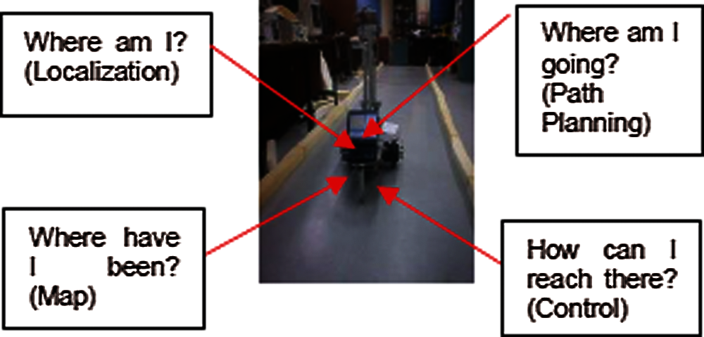
Figure 1: Autonomous mobile robot navigation processes
The environmental map involving the current and past environmental information interpreted by a global path planner was generally used in generating a low-resolution high-level path. Despite being an effective technique in finding an optimal path, it has some deficiencies when subjected to dynamic or hidden obstacles [7].
In local path planning algorithm, prior knowledge of the environment is not necessary. It solely provides from the onboard sensors a high-resolution low path in a fraction of global path information while working excellently in dynamic environments. In a tangled or long-distance environment, this method becomes ineffective [7]. In general, the path planning process for the current approach involves three main functions which are performed simultaneously [8,9]: (i) Sketch the robot's environment in a proper way. (ii) Find the collision-free path of the robot from the start to goal position and (iii) Search for the best optimum path to arrive to the goal. Other tasks such as following the rues, adhering to the constraints and recognizing the instructions are rare to be used in the current path planning algorithms.
Robot navigation is a process designed with the ability to avoid any hitch or obstacle to reach a certain position [10]. Path planning in robotic research is one of the most complicated problems that can occur during autonomous navigation in structured and unstructured environments, where the trajectory has to be planned continuously between the start and goal positions while attempting to avoid colliding with obstacles and other objects within the path [11]. A suitable approach will determine in the presence of obstacles the optimal path to the target within the shortest period of time.
Based on the reaction of the obstacles in the environment, it can further be classified as either offline or static and online or dynamic motion planning [12]. Path planning in robot methodologies are majorly classified in to two categories: Classical and the heuristics. Some of the popular classical methods include cell decomposition methods, subgoal method, potential field method, and sampling-based method. The heuristic methods include Neural network, Fuzzy logic and some nature inspired approaches including Genetic Algorithm (GA), Particle Swarm Optimization (PSO), and Ant-Colony Optimization (ACO). The problem of local minima and complexity associated with the classical methods render them practically inefficient. These problems are addressed by the heuristic approaches making them more applicable [13,14].
Optimal solutions are achieved in complex working environment with or without accurate information of the robot in some existed works. There have been numerous achievements in the area of robot path planning [15–18]. Most of the existing path-planning algorithms have been used within 2D-maps to search for the shortest path, determine the optimal-path to reach goal, avoiding static and dynamic obstacles and navigating a complex-environment. Nevertheless, none of these algorithms can be used in the maps of the constrained environments, where there are number of rules that must be strictly adhered.
The main contribution of this research is to propose a new path planning algorithm for robot navigation in both global and local environment to find the smoothest path within the shortest time from start to goal positions within a constrained environment. An additional optimization algorithm has been applied to find the most-optimum collision-free path by reducing the number of random points and the overall path length.
The current paper is organized as follows. Section 2 introduces some of the related works presented by researchers in the field of path planning. The methodologies proposed for mobile robot global and local path planning in this work are introduced in Section 3 while Section 4 demonstrates the effectiveness of the algorithm through a set of simulations in both local and global maps. Results were compared with two other previous works (A* and Laser simulator algorithm). Finally, Section 5 presents the conclusion of the obtained results.
Suppose the Mobile Robot (MR) moves from the Start Position (SP) to the Goal Position (GP) in an environment with static and dynamic obstacles to obtain certain performance criteria. The objective of a path planner is to find the optimal/near-optimal path for the mobile robot without any collision with obstacles exist within the environment.
There have been a lot of path planning methods (in both static and dynamic environments) proposed by researchers. Classical and heuristic approaches are the two major classes of path planning based on algorithmic classification [19]. Elshamli et al. [20] in his paper classified the path planning methods as exact and heuristic based on their completeness. According to the authors, an exact algorithm is the one which requires extensive/large computations to finds an optimal path planning solution while the heuristic algorithms are non-reliable in complex path planning problems as they find a solution to a path planning problem while limiting the computational time [20]. These approaches have both their weaknesses as well as advantages in different cases. Practical failure due to complexity in higher dimension and the problem of local minima are some of the disadvantages of the classical approaches [10]. However, these problems have been tackled rending the extensions in the application of heuristic approaches [21].
Studies by Stentz et al. [22], and Yu et al. [23] show that in a larger environment or situation in which the robots working environment need to be updated with a new information that requires re-planning, the computational cost is high while using this approach. Hence, some other re-planning methods in solving the problem of path changes have been proposed [24,25]. In [26], a variation of the A* algorithm named Fringe Saving A* (FSA*) algorithm was proposed for repeatedly finding a shortest path between the start and goal point in a known environment as the crossing path of the cells wavers up and down. This approach is faster as it utilizes the previous structure rather than starting from afresh. Another similar approach which uses an incremental heuristic search known as a Generalized Adaptive A* (GAA*) approach was proposed and presented in [27]. This approach modifies the consistent h(n) values to an upto-date h(n) value by updating the current search h(n) values with data obtained from the previous search thereby finding a short path even in time fluctuating action cost. Other proposed A* algorithms improvement strategies include Anytime Repairing A* (ARA*) [28], Dynamic Fringe-Saving A* [29], generalized Fringe Retrieving A* [25], and Lifelong Planning A* (LPA*) [30]. By adapting A* algorithm for a 3D representation of the robot's environment, Niu et al. [31] proposed an enhanced A* by introducing the idea of ‘cell’ and ‘region. A* and Theta* algorithm was implemented and compared by D. Filippis et al. [32] whose experimental results in 3D environment indicates higher search time in theta* than in the A* algorithm.
When there are lots of paths to get to the goal from the start point in a global and local environment, all previous methods will certainly attempt to stay clear of barriers and also look for the fastest path between the start and goal points [8]. The restrictions can be in the sorting rules which need to be purely adhered to within the path planning method. Owing to the restraints, the previous classical methods were unable to discover the ideal as well as risk-free course in the maps throughout navigating the constricted atmospheres such as manufacturing facilities as well as roadways. This was attributed to the following adhering to factors: (1) The framework of these methods were unable to make good sense or top priority to the restraints as well as having no mathematical formulas in the algorithms that can aid to approximate and place the restrictions. (2) The top priority in the algorithms is focusing on the computational time, the path length and also obstacle avoidance [9]. (3) The search-based methods were unable to handle the constricted environment given that the re-planning approach in these methods is constantly related to the obstacle avoidance. Also, objective searching comes without factors to consider to the restraints throughout the path finding [33–37]. (4) The AI based path planning on the other hand only takes some functions into factor to consider, specifically the fastest path, obstacle evasion and also global-local path planning [33–37]. To include restrictions in such formulas, it is required to create even more attributes to these algorithms, therefore enhancing the computational price as well as intricacy. To deal with the issue of constraints, many of the algorithms used in the existing automobile utilizes the Differential Global Positioning System (DGPS) signals with google maps.
3 Problem Statement, Motivation and Proposed Solution
A suitable path planning approach should determine the optimal path within the shortest period of time in the presence of obstacles. Optimal solutions are achieved in complex with/without accurate information of the robot's workspace environment. The path planning algorithms should address some challenges to overcome all conditions and uncertainties in real environments. These challenges can be summarized as follows:
1. It must follow the constraints and rules in the environments (increase intelligence)
2. It has a low computational cost (time consuming)
3. It has a low path cost (shortest path)
4. It finds an optimum path to reach the goal (one out of many paths to reach goal)
5. It is able to avoid collisions avoidance (obstacles)
However, none of the aforementioned approaches in section 2 except LS can deal effectively with challenge 1 (constrained environments such as roads and factories settings), where there are some rules and constraints that must be strictly adhered with. LS method presents a simulation and experimental evidence to drive robot in constrained environments. However it generates a zigzag path planning which is not suitable to be performed by mobile robot control system. Thus, a Generalized Laser Simulator is introduced in this paper to generate a smooth path in constrained environments with optimum, less computational, low path cost and avoiding obstacles. This paper will discuss in details the challenges 1–4, focusing on developing a novel algorithm for dealing with constraints in both local and global path planning. The algorithm can deal well with challenge 5, but it is out of scope of this paper and will be discussed in another paper.
4 Working Principle of Generalized Laser Simulator (GLS)
The main objective of a path planner is to find the most optimum path for the mobile robot from start to goal positions by following the rules, adhering with constraints and performing obstacles avoidance during autonomous navigation within the environment.
This section describes a novel method, called generalized laser simulator, to find the optimal or near optimal collision-free path. It is an improved method based on Laser Simulator method which has been successfully applied in many works [8,9] to deal with constraints and rules during path planning. The original laser simulator method depends on sending series of points as horizontal or vertical lines to detect the environment borders. On the other hand, a series of points that serve as waves are used in the generalized laser simulator method which helps to estimate the new path in all directions and thus enhancing the smoothness of the path. The proposed algorithm consists of three major steps:
1. Create a 2D grid map of the robot's workspace environment.
2. Develop a mathematical model for wave generation at GLS-first stage that produces the suitable candidate points for the path of the mobile robot in a constraint environment.
3. Develop an additional optimization technique at GLS-second stage that selects the best suited points in step 2 and construct an optimal path (as the obtained path is not optimal path in terms of the total path length, time and smoothness).
The first step of path planning is to model the workspace environment into suitable map representation. In GLS method, the environment is modelled into an image-based map with geometrical polygons shapes. In the global path planning, it is required to obtain the map information of the workspace environment before robot path planning, and then plan an optimal path from the start to the goal positions. The map is represented in two-dimensional (x, y) image, where x and y are coordinates in the map plane. The concept of GLS path determination involves the use of the following specifications and assumptions in regards with workspace modelling:
1. The search environment is modelled in two dimensional state space X (x, y) and the surrounding environments borders are represented as polygons.
2. The robot's Cartesian coordinate system of the initial position S (xs, ys) and final position G (xg, yg) are known.
3. The robot can relocate to a free space in any direction in a time.
4. There are no other effects acting on the robot except the obstacles and constraints
4.2 GLS-First Stage: Waves Generation
The GLS method depends on generating a series of points as waves, starting from an initial position to target point, to detect the border of the environment and find the new position of the robot path. The waves will spread out until it hit the borders of the environment, i.e., the generations of waves will not be stopped until detecting the map borders as shown in Fig. 2.
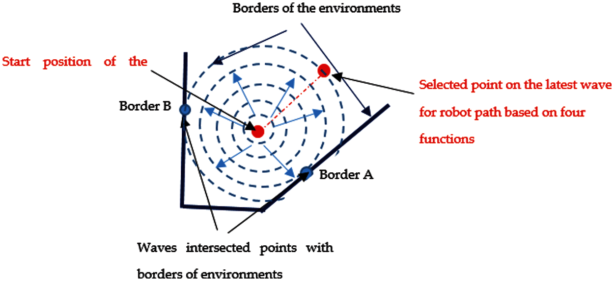
Figure 2: An overview of the GLS method
The wave must detect at least two borders to determine the robot path. However if the wave detects only one border of the environment (denoted A in Fig. 2), it will continue spreading out until detecting the second borders (denoted B in Fig. 2). The number of borders detected in the map is remarked by flag, e.g., flag = 2 means the algorithm is able to detect two borders. It is considered here the ideal case of wave generation where it spreads as a circle shape. As there are many points and directions on the latest wave (The wave that is intersected with the environment borders) to reach the goal, the selection of path point will be based on four main criteria, namely: reaching the goal, avoiding obstacles, adhering with constraints and shortest path to reach goal as will be explained in next sections and shown in Fig. 2.
In order to generate the waves in effective way, 8 points (45 degrees apart) that form the wave circumference in four directions, namely; Top Row, Left Column, Right Column and Bottom Row as shown in Fig. 3a are used. These points are represented in the constructed map as 8 pixels, which are checked after that to see whether it is dark or white color. A darker color value indicates that a border of an environment has been detected. The number of pixels to be scanned is determined using Eq. (1).
where Nr is the number of interest points per round and n is the wave number. Eq. (2) are used to determine the Cartesian coordinate values for each point in the top row, bottom row, right column and left column of the wave as shown in Fig. 3b.
where x and y are the center position of wave, R is the radius of the wave in pixels which will be incremented when it goes from the smallest to the biggest waves by 5–10 pixels. α is the angle of the points location with regard to the center of the wave (it is equal to 450 between each two points).
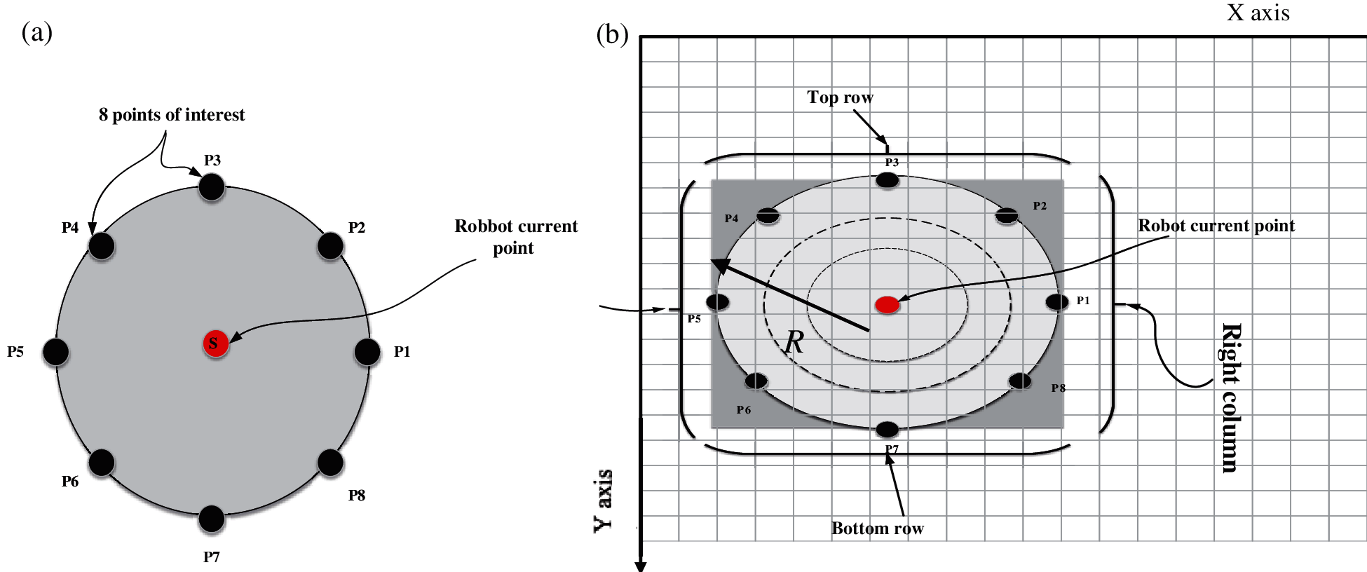
Figure 3: Index of interest for the generated waves: (a) Generation of 1st waver (b) Generation of other waves
To find the best candidate of the points, two concepts have been implemented:
–The concept of minimum distance to the goal point
–The maximum distance from to the nearest boundary.
The algorithm keeps generating waves when flag is less than two until it reaches a value of two (i.e., out of the four boarders it reaches two borders at least).
4.2.1 The Concept of Minimum Distance to the Goal Point
This minimum distance method checks the candidate points and finds out whichever amongst of them has the lowest distance to the goal position as shown in Fig. 4a. On this note, the concept of probability of the minimum distance has been introduced to generate the most preferred point to move. The distance between the points and goal position is calculated using Eq. (3).
The minimum distance is calculated using Eq. (4):

Figure 4: Generalized Laser Simulator approach (a) Minimum distance approach (b) Distance from boundary approach
As the points are not correlated with each other, the probability of each point is calculated using Eq. (5):
The probability of the preferred point is calculated using Eq. (6):
It is also required to use another criterion before selection of the right path of the robot which is based on the index distance from a boundary. From start point, one can determine how much is the distance from the nearest boundaries in the right, left, top and bottom direction to the path's candidate point as shown in Fig. 4b. It uses the concept of probability of maximum distance as in Eq. (6) to find the most suitable point for the robot path, in which the highest probability is preferred.
4.2.2 The Maximum Distance to the Nearest Boundary
To calculate the distance between the 8th points and border in all directions, Eq. (7) is used:
The maximum distance is calculated using Eq. (8):
Similar to the previous case, the points are not correlated with each other, thus the probability of each point is calculated using Eq. (9).
To qualify the point as a candidate for the robot path, it must fulfill both of the following criteria:
–It has minimum distance to the goal point
–It has maximum distance from to the nearest boundary.
The best suited candidate point for the path is calculated based on the summation of probability in Eqs. (6) and (9). Eqs. (10) and (11) are used to calculate the best suited candidate point for the path:
4.3 GLS Second Stage: Path Candidate Sellection and Optimization
This section introduces the path candidate selection and optimization method used to generate the shortest path from the whole candidate points that have been determined in the first stage. The optimized GLS is used to reduce the number of path points of the GLS between the start and goal points to obtain an optimal path. As shown in Fig. 5a, the path points are represented by red circle objects, and the obtained shortest path (optimized) is represented by a thick blue line as in Fig. 5b.

Figure 5: Path Planning: (a) Points obtained by GLS (b) shortest path after optimization
In the optimization stage, it is aimed to find out the minimum distance the robot can move without colliding with any obstacle.
The optimization process starts by identifying the position of the current and chosen points. This is followed by arranging of all x values of the chosen points as a vector X based on ascending procedure. The same goes to y values, which are arranged as vector Y that contain the ascending values in y direction. The distance of all other points to the goal point are calculated in order to determine the minimum distance amongst all of them, taking note of the goal position with respect to the start point. If the goal is above to the start position, then they are in an incremental order. Otherwise, if the goal is below the start point then they are in a decrement order. So, by this way, the coordinate values in x and y directions are sorted for the selected points from start position with either increment or decrement to reach the goal position. Next, the current point is compared to the new chosen point to find if these points are matched which would result in ignoring to move to that point. In the case of mismatch, then the possibility of moving to next chosen point is checked without crossing a border or boundary. If there is no border, the robot will move to next chosen point, taking note that if there is an obstacle, the next chosen point is removed. In the case that there are obstacles between current and all next chosen points, one can just choose the 1st chosen point.
4.4 Constraints Representation
The constraints are used to describe the rules that are needed to be followed during the path finding process. If there are multiple paths in which the proposed algorithm could pass through to reach the target, the GLS will evaluate all the paths based on three criteria, namely; constraints function Eq. (13) and distances of the wave's candidate points to the target and borders (up, left, down and right borders) as discussed in sections 3.2.1 and 3.2.2. A series of waves are generated from the current position to detect at least two borders of environments with a maximum of 20 waves. In the case that it exceeds 20 waves without detecting the borders, the algorithm will choose the 1st point among the 8th points of the wave circumference.
The constraint function is activated if the flag value after twenty wave generation is less than two as is illustrated using the corridor environment in Fig. 6. Consider the situation at position point 1 in Fig. 6 where the possible interesting indexes are within the up and right borders. By applying the two criteria mentioned above for the distance of points to goal and borders, the points within the upward border will be discarded as they will make the distance to goal longer, and the proposed algorithm will process to find the next point. Waves are generated with the 8 interesting points which are continuously compared with 255 grey scale. If any of among these points is in range of (0–50), its value is recorded as black pixel (border of environment) and the flag is incremented. If the flag value is one, the program will continue as it needs to reach at least flag value of 2 to stop. When the flag value reaches two, the algorithm moves to the next stage. However, during the second iteration at point 2 as seen in Fig. 10, the interesting indexes are in in the directions up, right and down. In such case, the constraints function will be activated and the proposed algorithm will switch its pattern.
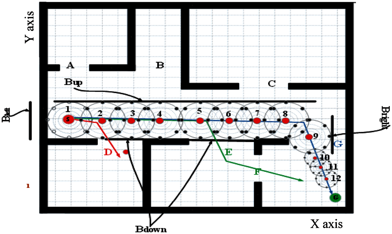
Figure 6: Constraints identification
The constraint function F(CR) is given by Eq. (12)
where F(CR1) is a function related to the number of waves generation per round (it is considered as 20 waves per round and the number of borders that should be detected is at least 2 borders). It can be activated when its value is 1 and deactivated when the value is 0 as in Eq. (13):
F(CR2) is a function related to non-visited points. It can be given value 1 if the point is not previously visited as in Eq. (14):
F(CR3) is a function related to the minimum distance to reach the goal. It can detect the direction of constraints in the left, right, up and down sides as in Eq. (15).
where dminis the minimum distance to reach the goal as in Eq. (4).
5 GLS Implementation in Local and Global Path Planning
The practical and simulation implementation of the proposed algorithm in both indoor and outdoor 2D-maps environments is presented in this section. It is implemented in two types of environments, namely; global and local environments. In the global environment, the map is completely known and the robot must move towards its goal within shortest path, smoothness path and adhering with constraints. In the local path planning, the mobile robot is supposed to navigate on the environment in real-time and reach the pre-determined goal while discovering and detecting the boundaries, constraints and finding the shortest path.
In this study, the proposed method has been tested under a series of simulations in 2D maps to exhibit its effectiveness. The resolution of maps is 500 × 500 pixels and all simulations were coded and run on MATLAB R2014b (64-bit win64) on a laptop with Intel(R) core (TM) i5 − 2450 M. The performances of the developed method have been tested on many different workspace scenarios with the presence of constraints. The starting and the goal points have been positioned in different locations within the map's free space.
The red and green points signify the start (S) and goal positions (G), respectively. The algorithm was simulated in each environment 30 times. The simulation results of GLS and optimized GLS are presented in the next subsections. Additionally, the performance of the proposed method is compared with the other paths algorithms.
It includes the result of GLS in the first (wave generations) and second stages (optimization process) as follows:
5.1.1 GLS Results Without Optimization
This sub-section presents the results of the proposed algorithm for generating feasible path between start and the goal points for all the workspace scenarios in 20 different environments (A-T) shown in Fig. 7. The achieved result of the proposed algorithm is represented by a set of path points p(i), (i = 1 → T). Each new position of waypoint w (i + 1) is allocated after the current path points position w(i), where T represents the time in which the robot reaches the goal point. The simulation results for all the tested scenarios are presented in Fig. 7.
From Fig. 7, it is observed that the obtained GLS allows the robot to move from start to goal locations from/to any position in the workspace. The path points are represented as red points and are connected by a continuous path. Each of these environments is simulated for 30 trials which show clearly that the proposed method provides suitable collision-free path for the robot.
5.1.2 Simulation Results of GLS-Second Stage (Optimization)
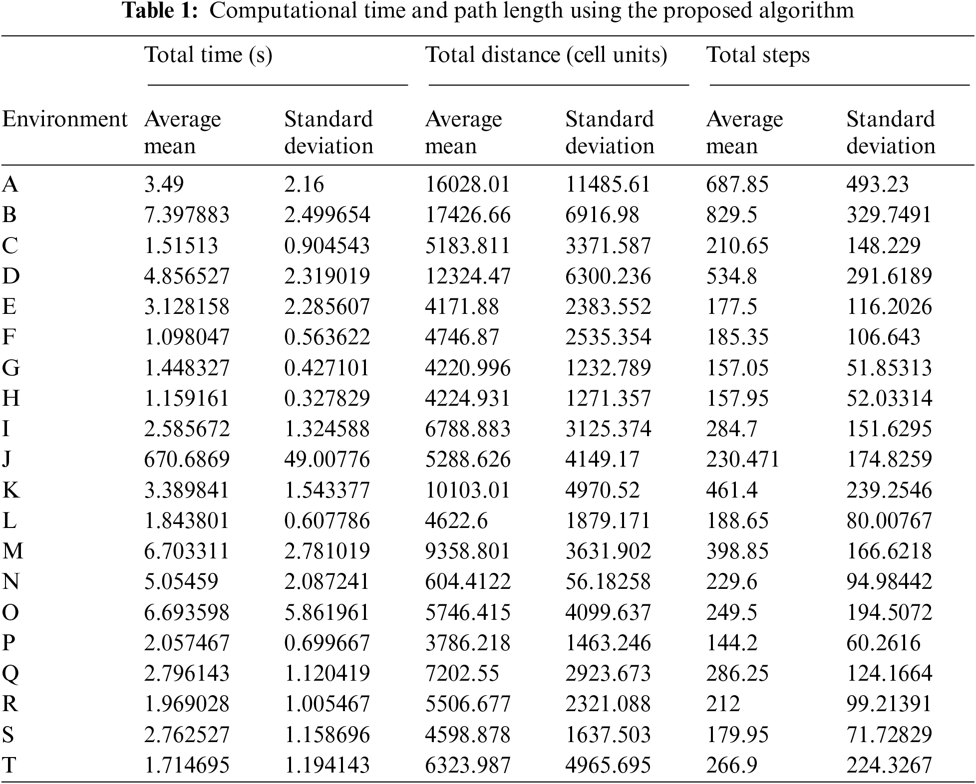
The previous generated paths in Fig. 7 are not optimal in terms of the total path length, time and smoothness. In order to reduce the overall path length, the proposed algorithm is further optimized, and the results of path determination of environments (A-T) are presented in Fig. 8. The arrival time and path length for every run are mentioned in Tab. 1. The proposed algorithm created safe and short paths within reasonable arrival time.
5.1.3 Comparisons with Other Algorithms
In order to validate the efficiency of the proposed algorithm, the proposed algorithm performance was compared with LS and A* method which are closely related to the proposed study in many aspects. To assess the performance of the proposed algorithm, five different scenarios of 2D environments are used, in which each scenario is planned using the three algorithms and the results of them are then compared. Fig. 9 shows five different environments (A-E), in which three path planning algorithms were used to generate the path: (1) Laser simulator (LS) as shown in Fig 9a for environments A, B, C, D and E (2) A* as shown in Fig. 9b for environments A, B, C, D and E and (3) Generalized Laser Simulator (GLS) as shown in Fig. 9c for environments A, B, C, D and E.

Figure 7: Results of GLS-first stage (wave generation)
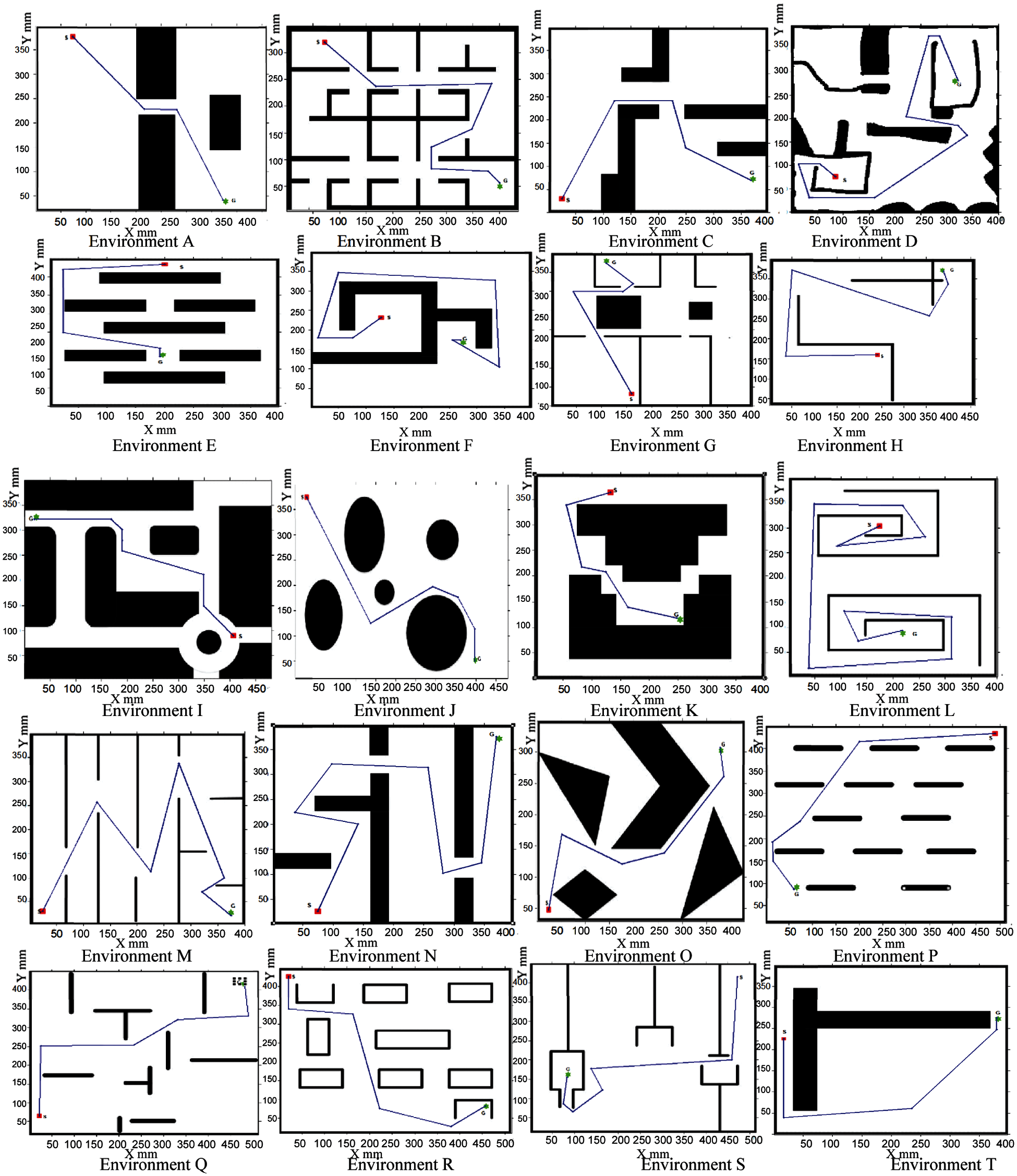
Figure 8: Final path after GLS second stage (optimization)
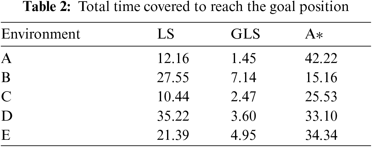
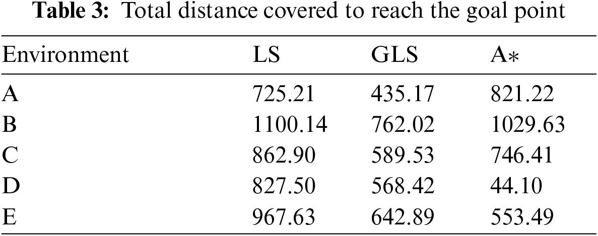
The specific quantitative analysis comparison between the algorithms in terms of computational time is illustrated in Tab. 2. From Tab. 3, the performance of LS, GLS and A* methods were compared in terms of path length. Fig. 10a shows the comparison of running time between LS, GLS, and A* methods for four environments (name it) with two different start and goal positions. Fig. 10b displays the comparisons of path length of LS, GLS, And A* methods for the same four environments with two different start and goal position. From Fig. 10, it can be clearly seen that the running time of A* is much greater than LS while the proposed algorithm demonstrates the smallest running time. Also, one can see that the path length of LS is longer than A*, and the path length of A* is larger than the proposed algorithm. As for average time in Tab. 2, GLS is faster than A* and LS by 7.8 and 5.5 times, respectively. As for average distance in Tab. 3, GLS presents a path which is shorter than A* and LS by 1.2 and 1.5 times, respectively.
It can be clearly concluded that the GLS has the best performance in both path length and computational time over all algorithms. In addition, the path of GLS is much smoother in comparison with A* and LS as shown in Figs. 9 and 11.
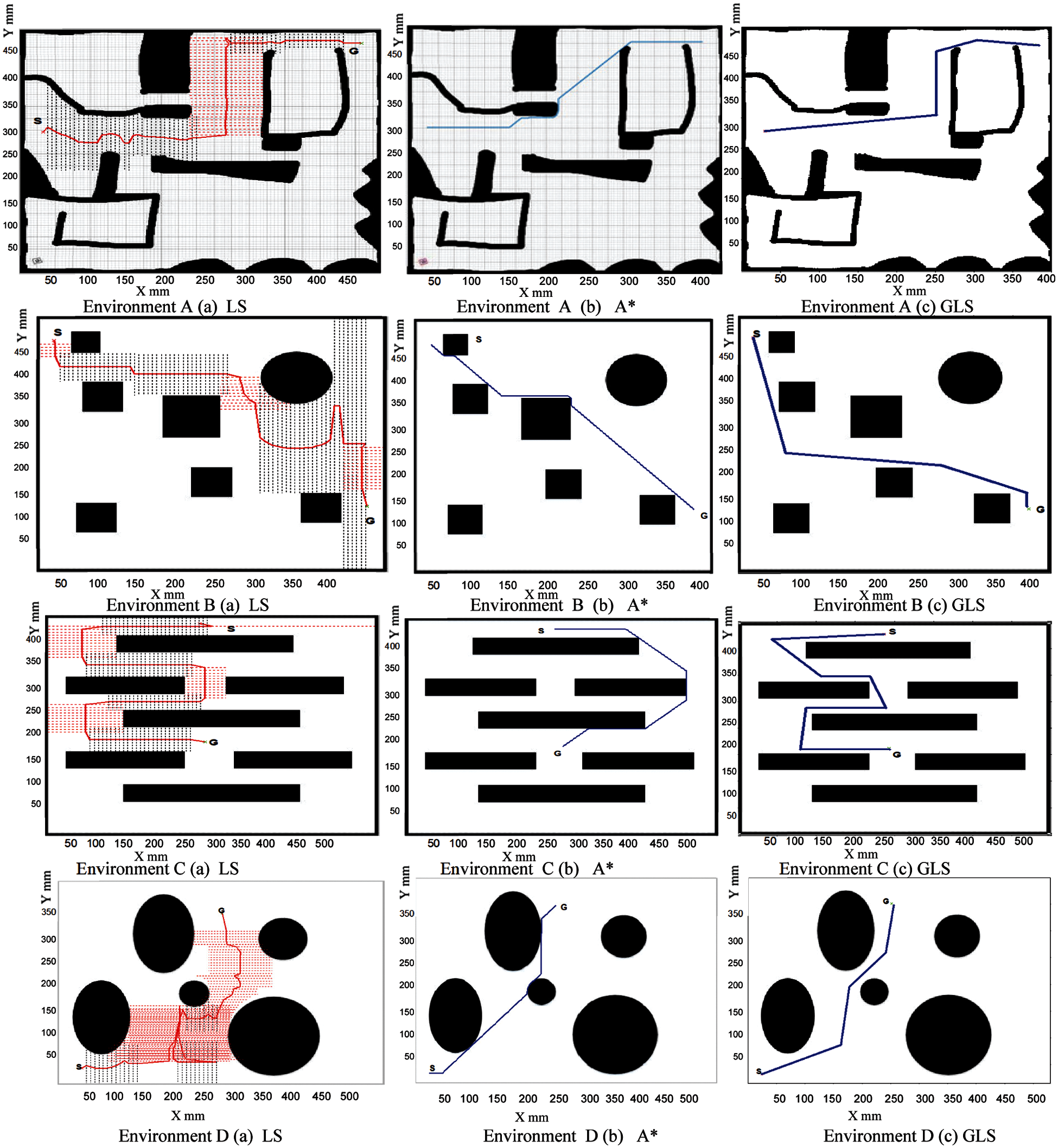
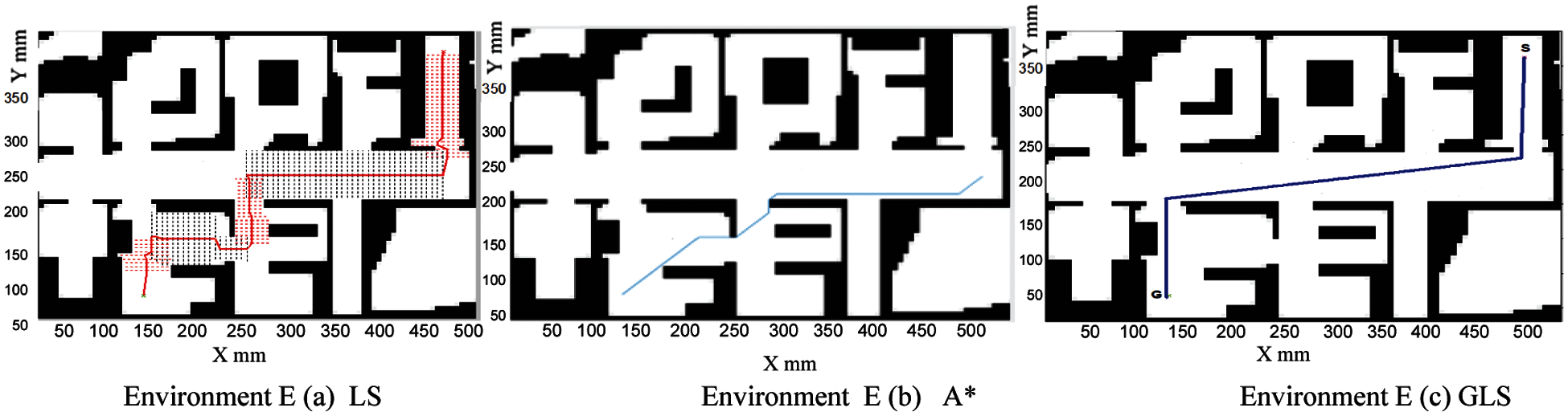
Figure 9: Comparison between Laser Simulator, A* and Generalized Laser simulator in several environment Environment A (a) LS Environment A (b) A* Environment A (c) GLS Environment B (a) LS Environment B (b) A* Environment B (c) GLS Environment C (a) LS Environment C (b) A* Environment C (c) GLS Environment D (a) LS Environment D (b) A* Environment D (c) GLS Environment E (a) LS Environment E (b) A* Environment E (c) GLS
The GLS and A* algorithms were both simulated in 2D-maps as shown in Fig 11, to show its effectiveness in adhering with constraints. As seen in Fig. 11, the GLS algorithm is able to identify the constraints path which is to follow the corridor until it reaches the goal point. The A* algorithm reaches the goal position while searching for any shortest path without consideration to go in the corridor.

Figure 10: Comparison between GLS, LS, A*: (a) time to goal in Environment A (b) Distance to goal in Environment A

Figure 11: Constriants comparison between Proposed algorithm GLS and A* algorithm in two environments
5.2 Real-Time Path Planning Results
The GLS approach was used for road environments detection within the indoor and outside environments to generate the path of the robot and localize it within its terrain. The local maps were built using camera to estimate the road border parameters such as road width and curbs in 2D. A Wheel Mobile Robot as shown in Fig. 12 is used for the indoor and outdoor navigation. The platform includes three main units: differential drive unit, measurement and vision unit and processing unit. The sensors, actuators and the interface free controller cards are connected together in such a way that ensures high performance for exchanging the data from the on-board computer to the sensors and actuators. The embedded controller of the proposed platform has been developed to integrate the mechanical components with electronics and software algorithms. The proposed GLS is able to navigate autonomously on both indoor and outdoor applications.
Robot is able to find the path starting from the pre-defined start pose until it reaches the pre-goal position using the GLS approach for the local map that was identified by the camera.

Figure 12: Developed WMR platform that is used in the experiments that shows (a) the outer parts on the platform (b) the inner parts
The pre-processing and processing operations are applied to prepare the images for LS and GLS path planning as shown in Figs. 13b–13d. In each frame's image, the GLS is used to investigate the number of pixels between the environment borders. The indoor navigation results show the capability of the LS and GLS algorithms to generate the path on the image after processing in the presence of constrains from the sequences of frames as shown in Fig. 13. Fig. 13a presents the original image while Figs. 13b and 13c show the post processing path obtained by the LS and GLS in respectively. The final path obtained using the GLS is shown in Fig. 13d.
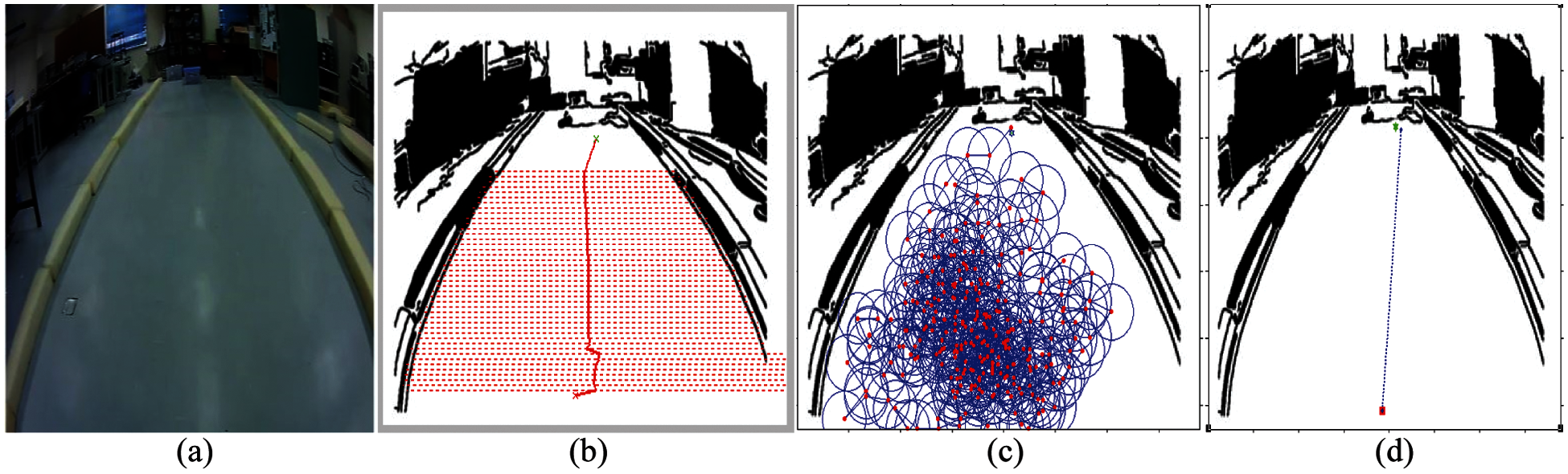
Figure 13: Indoor navigation with no obstacle on the road (a) original image (b) applying LS algorithm (c) applying GLS (d) final path of GLS
The GLS algorithm was applied to a real road roundabout in Universiti Malaysia Pahang (UMP) campus. The robot or autonomous vehicle has to adhere to the rules of the roundabout and chooses the right outlet of the roundabout according to the goal position. Thus, it needs a high evidence path planning algorithm to navigate the robot through the roundabout by following the required constraints. Figs. 14 and 15 show that GLS is able to drive the robot in a roundabout environment and adhering well with constraints.
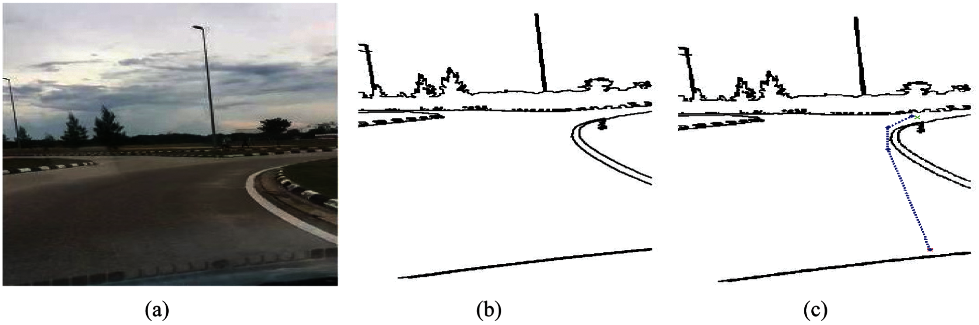
Figure 14: Results of outdoor path planning: (a) original images (b) images from the pre-processing and processing operations (c) applying the GLS
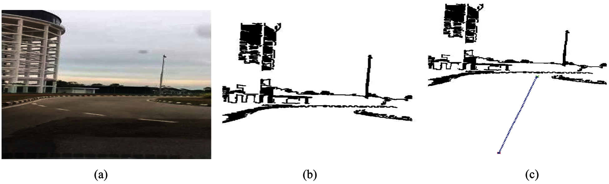
Figure 15: Results of outdoor path planning: (a) outdoor planning: original images (b) images from the pre-processing and processing operations (c) applying the GLS
In this paper, a novel algorithm, called Generalized Laser simulator, has been developed for solving path planning problem of a mobile robot in a two-dimensional constrained working environment under the presence of constraints. GLS algorithm is guaranteed to find an optimal path for a mobile robot through a sequence of waves that enable the robot to move in a known or unknown environment from the starting point to the goal point by adhering to any constraint. For this purpose, the proposed GLS builds all feasible paths between any arbitrarily selected start and goal locations in a discrete gridded environment within the first stage. It follows by an optimal collision-free path determination stage through reducing the number of path points and selecting the optimum path. In order to validate the performance of the developed method in comparison with existing path planning methods, a comparative study between the proposed algorithm, LS and A* in several different environmental scenarios with different complexity have been performed. Path length, smoothness, constraints, and time were considered as comparison parameters to evaluate the quality of the obtained paths. The comparison reveals that the proposed method can solve the path planning problem effectively and efficiently in terms of the computational times and the path length with smoothness path. In comparison to deterministic path planning algorithms like Laser simulator and A∗, it can be said that the proposed algorithm is able to find the best piecewise linear path. The two advantages of the proposed algorithm in comparison to the compared algorithms are time efficiency and the ability to find optimal path in any complex environment. As such, the proposed algorithm can be considered as a significant contribution to the field of expert and intelligent systems for mobile robot path planning. As a future work, the proposed algorithm should be extended to solve the multi-robot path planning problem in both 2D and 3D environments.
Funding Statement: The authors would like to thank the United Arab Emirates University for funding this work under Start-Up grant [G00003321].
Conflicts of Interest: The authors declare that they have no conflicts of interest to report regarding the present study.
1. Y. Q. Qin, D. B. Sun, N. Li and Y. G. Cen, “Path planning for mobile robot using the particle swarm optimization with mutation operator,” in Proc. Conf. on Machine Learning and Cybernetics, Shanghai, China, pp. 2473–2478, 2004. [Google Scholar]
2. P. Raja and S. Pugazhenthi, “Optimal path planning of mobile robots: A review,” International Journal Physical Sciences, vol. 7, no. 9, pp. 1314–1320, 2012. [Google Scholar]
3. Y. Zhao, Z. Zheng and Y. Liu, “Survey on computational-intelligence-based UAV path planning,” Knowledge-Based Systems, vol. 158, no. 2018, pp. 54–64, 2018. [Google Scholar]
4. H. Zhang, J. Butzke and M. Likhachey, “Combining global and local planning with guarantees on completeness,” in Proc. IEEE Conf. on Robotics and Automation, Saint Paul, MN, USA, pp. 4500–4506, 2012. [Google Scholar]
5. L. C. Wang, L. S. Yong and M. H. Ang, “Hybrid of global path planning and local navigation implemented on a mobile robot in indoor environment,” in Proc. IEEE Int. Symposium on Intelligent Control, Vancouver, BC, Canada, pp. 821–826, 2002. [Google Scholar]
6. Z. Bi, Y. Yimin and Y. Wei, “Hierarchical path planning approach for mobile robot navigation under the dynamic environment,” in Proc. IEEE Conf. on Industrial Informatics, Daejeon, Korea (Southpp. 372–376, 2008. [Google Scholar]
7. M. A. H. Ali, M. Mailah, K. Moiduddin, W. Ameen and H. Alkhalefah, “Development of an autonomous robotics platform for road marks painting using laser simulator and sensor fusion technique,” Robotica, vol. 39, no. 3, pp. 535–556, 2021. [Google Scholar]
8. M. A. H. Ali and M. Mailah, “Laser simulator: A novel search graph-based path planning approach,” International Journal of Advanced Robotic System, vol. 15, no. 2018, pp. 1–16, 2018. [Google Scholar]
9. M. A. H. Ali and M. Mailah, “Path planning and control of mobile robot in road environments using sensors fusion and active force control,” IEEE Transactions on Vehicular Technology, vol. 68, no. 3, pp. 2176–2195, 2019. [Google Scholar]
10. F. Kamil, S. H. Tang, W. Khaksar, N. Zulkifli and S. A. Ahmad, “A review on motion planning and obstacle avoidance approaches in dynamic environments”. Advances in Robotics & Automation, vol. 4, no. 2, pp. 1–8, 2015. [Google Scholar]
11. L. Wang, “Path planning for unmanned wheeled robot based on improved ant colony optimization,” Measurement and Control, vol. 53, no. 5–6 pp. 1014–1021, 2020. [Google Scholar]
12. M. A. H. Ali, M. Mailah, W. A. Jabbar, K. Moiduddin, W. Ameen et al., “Autonomous road roundabout detection and navigation system for smart vehicles and cities using laser simulator– fuzzy logic algorithms and sensor fusion,” Sensors, vol. 20, no. 13, pp. 1–26, 2020. [Google Scholar]
13. E. Masehian and D. Sedighizadeh, “Classic and heuristic approaches in robot motion planning-a chronological review,” International Journal of Mechanical, Industrial Science and Engineering, vol. 1, no. 5, pp. 255–260, 2007. [Google Scholar]
14. S. H. Tang, W. Khaksar, N. B. Ismail and M. K. A. Ariffin, “A review on robot motion planning approaches,” Pertanika Journal Science and Technology, vol. 20, no. 1, pp. 15–29, 2012. [Google Scholar]
15. Z. A. Ali, H. Zhangang and R. J. Masood, “Collective motion and self-organization of a swarm of UAVs: A cluster-based architecture,” Sensors, vol. 21, no. 11, pp. 1–19, 2021. [Google Scholar]
16. S. Li, Y. Zhang and L. Jin, “Kinematic control of redundant manipulators using neural networks,” IEEE Transaction on Neural Networks and Learning System, vol. 28, no. 10, pp. 2243–2254, 2017. [Google Scholar]
17. D. Chen and Y. Zhang, “Hybrid multi-objective scheme applied to redundant robot manipulators.” IEEE Transactions on Automation Science and Engineering, vol. 14, no. 3, pp. 1337–1350, 2017. [Google Scholar]
18. D. Guo, F. Xu and L. Yan, “New pseudoinverse-based path-planning scheme with PID characteristic for redundant robot manipulators in the presence of noise,” IEEE Transactions on Control Systems Technology, vol. 26, no. 6, pp. 2008–2019, 2018. [Google Scholar]
19. A. Chakravarthy and D. Ghose, “Obstacle avoidance in a dynamic environment: A collision cone approach,” IEEE Transactions on Systems, Man, and Cybernetics - Part A: Systems and Humans, vol. 28, no. 5, pp. 562–574, 1998. [Google Scholar]
20. A. Elshamli, H. A. Abdullah and S. Areibi, “Genetic algorithm for dynamic path planning,” Canadian Conf. on Electrical and Computer Engineering, pp. 677–680, Niagara Falls, ON, Canada: IEEE, 2004. [Google Scholar]
21. M. A. H. Ali, M. Mailah and T. H. Hing, “Implementation of laser simulator search graph for detection and path planning in roundabout environments,” WSEAS Transaction on Signal Processing, vol. 10, no. 2014, pp. 118–126, 2014. [Google Scholar]
22. A. Stentz, “The focussed D* algorithm for real-time replanning,” in Proc. Int. Joint Conf. on Artificial Intelligence, Montreal, Quebec, Canada, pp. 1–8, 1995. [Google Scholar]
23. H. Yu, C. J. Chi, T. Su and Q. Bi, “Hybrid evolutionary motion planning using follow boundary repair for mobile robots,” Journal of System Architecture, vol. 47, no. 7, pp. 635–647, 2001. [Google Scholar]
24. S. Koenig and M. Likhachev, “Improved fast replanning for robot navigation in unknown terrain,” in Proc. IEEE Int. Conf. on Robotics and Automation, Washington, DC, USA pp. 968–975, 2002. [Google Scholar]
25. X. Sun, W. Yeoh and S. Koenig, “Generalized fringe-retrieving A*: faster moving target search on state lattices,” in Proc. Int. Conf. on Autonomous Agents and Multiagent Systems, Toronto, Canada, pp. 1081–1088, 2010. [Google Scholar]
26. X. Sun and S. Koenig, “The fringe-saving A* search algorithm — a feasibility study,” in Proc. 20th Int. Joint Conf. on Artificial Intelligence, Hyderabad, India, pp. 2391–2397, 2007. [Google Scholar]
27. X. Sun, S. Koenig and W. Yeoh, “Generalized adaptive A*,” in Proc. Int. Conf. on Autonomous Agents and Multi-Agent Systems, Estoril, Portugal, pp. 1–8, 2008. [Google Scholar]
28. M. Likhachev, D. Ferguson, G. Gordon, A. Stentz and S. Thrun, “Anytime search in dynamic graphs,” Artificial Intelligence, vol. 172, no. 14, pp. 1613–1643, 2008. [Google Scholar]
29. X. Sun, W. Yeoh and S. Koenig, “Dynamic fringe-saving A*,” in Proc. 8th Int. Joint Conf. on Autonomous Agents and Multi-Agent Systems, Budapest, Hungary, pp. 1–9, 2009. [Google Scholar]
30. S. Koenig, M. Likhachev and D. Furcy, “Lifelong planning A*,”Artificial Intelligence, vol. 155, no. 1–2, pp. 93–146, 2004. [Google Scholar]
31. L. Niu and G. Zhuo, “An improved real 3d A∗ algorithm for difficult path finding situation,” in Proc. Int.,A rchives of the Photogrammetry, Remote Sensing and Spatial Information Sciences, Beijing, China, pp. 927–930, 2008. [Google Scholar]
32. L. D. Filippis, G. Guglieri and F. Quagliotti, “Path planning strategies for UAVS in 3D environments. Journal of Intelligent and Robotic System, vol. 65, no. 2012, pp. 247–264, 2012. [Google Scholar]
33. J. Meijer, Q. Lei and M. Wisse, “An empirical study of single-query motion planning for grasp execution,” in Proc. IEEE Int. Conf. on Advanced Intelligent Mechatronics, Munich, Germany, pp. 1234–1241, 2017. [Google Scholar]
34. A. Gasparetto, P. Boscariol, A. Lanzutti and R. Vidoni, “Path planning and trajectory planning algorithms: A general overview,” Motion and Operation Planning of Robotic System, vol. 29, no. 2015, pp. 3–27, 2015. [Google Scholar]
35. B. Zhu, C. Li, L. Song, Y. Song and Y. Li, “A∗ algorithm of global path planning based on the grid map and V-graph environmental model for the mobile robot,” in Proc. Chinese Automation Congress, Jinan, China, pp. 4973–4977, 2017. [Google Scholar]
36. M. A. H. Ali, M. S. A. Radzak, M. Mailah, N. Yusoff, B. A. Razak et al., “A novel inertia moment estimation algorithm collaborated with active force control scheme for wheeled mobile robot control in constrained environments,” Expert Systems with Applications, vol. 183, no. 2021, pp. 1–29, 2021. [Google Scholar]
37. Z. A. Ali, H. Zhangang and W. B. Hang, “Cooperative path planning of multiple UAVs by using max–min ant colony optimization along with Cauchy mutant operator,” Fluctuation and Noise Letter, vol. 20, no. 1, pp. 2150002, 2021. [Google Scholar]
 | This work is licensed under a Creative Commons Attribution 4.0 International License, which permits unrestricted use, distribution, and reproduction in any medium, provided the original work is properly cited. |